14 Curvilinear Motion, Motion of a Projectile

14
Curvilinear Motion, Motion of a Projectile
Ref: Hibbeler § 12.6, Bedford & Fowler: Dynamics § 2.3
Rectilinear motion refers to motion in a straight line. When a particle follows a non-straight path, it’s
motion is termed curvilinear. Projectile motion is typically curvilinear, although a projectile fired
straight up (in the absence of a crosswind), or moving along a straight track would be rectilinear
motion.
A projectile’s motion can be broken down into three phases: an acceleration phase where the
actuator (gun, catapult, golf club, etc.) gets the projectile moving. The second phase of motion is after
the projectile leaves the actuator, when the only acceleration acting on it is the acceleration due to
gravity.
Note: A common assumption that simplifies the problem considerably, but is not altogether accurate,
is that the frictional drag between the projectile and the fluid through which it moves is negligible. This
assumption is more reasonable for small, smooth, slow-moving particles through low-viscosity fluid
than for large, irregularly shaped particles moving at high speeds through highly viscous fluids.
The third phase of a projectile’s motion is after impact. The particle may roll, continue moving through
a very different medium (water or earth), or break up. Here we will consider only the second phase of
the projectile’s motion: the projectile has already been accelerated by an actuator, and is flying
through the air.
Example: Slingshot Contest
Projectile throwing contests are pretty common at engineering schools. There are several ways to run
the contest: highest, farthest, most accurate, etc; and several ways to propel the projectile: slingshot,
catapult, etc. This example focuses on a tennis ball slingshot competition.
Tennis Ball Data (approximate)
Diameter
2.5 inches (6.4 cm)
Weight 2 oz (57 g)
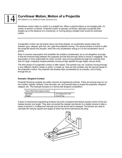
A team of mechanical engineering students has built a slingshot that allows precise control of the prerelease
tension and angle. They also connected the release mechanism to a digital camera to take a
series of photos in 1millisecond intervals just as the tennis ball is released. The photos are used to
calculate the velocity (speed and angle) at which the tennis ball leaves the sling.

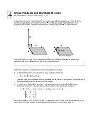
A test run with the camera operational gave the following set of photos (superimposed).
25°
0 20 40 60 mm
Part 1.
Determine:
a. The initial velocity of the tennis ball as it leaves the sling.
b. The predicted time of flight for the ball.
c. The predicted horizontal travel distance for the ball.
Part 2.
The team that gets most balls into a basket set 30 meters from the launch site wins. If they can keep
the initial speed constant (at the test run value of 22.1 m/s), what angle should they use to shoot the
tennis balls into the basket?
Part 1. Solution
The initial velocity is calculated from the 60 mm horizontal travel distance observed in the photos
using the camera’s 1 millisecond interval between snapshots.
» x_test = 60 / 1000; %Horizontal travel distance for all four frames (m)
» theta = 25 * pi/180; %Angle of trajectory (radians)
» d_test = x_test / cos(theta) %Distance ball traveled in direction of motion (m)
d_test =
0.0662
» dt_pic = 0.001; %Interval between snapshots (s)
» dt_test = 3 * dt_pic; %3 time intervals between the four photos
» v_int = d_test / dt_test %Initial velocity of the tennis ball
v_int =
22.0676
The horizontal and vertical components of the initial velocity will be useful for later calculations.
» v_yint = v_int * sin(theta) %y component of initial velocity

v_yint =
9.3262
» v_xint = v_int * cos(theta) %x component of initial velocity
v_xint =
20
» v_x = v_xint %x component of velocity is constant (if air resistance is ignored)
v_x =
20
The predicted time of flight can be calculated using
1
2
0 + v y _ init t flight a
2 c t flight
y = y
+
where a c is the constant acceleration. In this problem, the acceleration is due to gravity and acts in
the –y direction, so a c = -g.
If we assume that the flight is over a horizontal surface, then y at the end of the flight is zero. Another
common assumption is to assume that y 0 is also zero. This is a reasonable assumption if the vertical
position of the tennis ball as it leaves the sling is small compared to the maximum height reached
during the flight.
With these assumptions, the equation can be solved for the time of flight
t
flight
−2 v
=
a
y _ init
c
Using MATLAB, the time of flight is predicted to be 1.9 seconds.
» a_c = -9.8; %The constant acceleration in this problem is due to gravity
» t_flight= -2 * v_yint / a_c
t_flight =
1.9033
We can calculate the maximum height to see if the assumption that y 0 is negligible is reasonable. The
maximum height occurs at ½ the flight time (if y 0 =y final , and air resistance is negligible).
» y_o = 0;
» y_final = 0;
» y_max = y_o + v_yint * t_flight / 2 + a_c / 2 * ( t_flight/2 )^2
y_max =
4.4376
Looking at the drawing of the slingshot, the ball is released at a height about two or three times the
ball diameter, around 15 to 20 cm. 20 cm is nearly 5% of y max . That is probably negligible, but we can
use MATLAB’s root finder to find t flight including y 0 = 20 cm.

» y_o = 20 / 100; %Initial height (m)
» y_final = 0; %Final height (m)
» coeffs = [( a_c/2 ) ( v_yint ) ( y_o - y_final )]; %Polynomial
» t_flight= roots(coeffs) %Roots
t_flight =
1.9245
-0.0212
» t_flight= t_flight(1) %Choose positive root
t_flight =
1.9245
Note: See the annotated MATLAB Script Solution for a more complete explanation of MATLAB’s
roots function and how MATLAB represents polynomials.
Accounting for the initial height increased the predicted flight time from 1.902 to 1.925 seconds (about
1% difference).
Finally, we calculate the predicted horizontal travel distance.
» x_o = 0; %Initial horizontal position
» x = x_o + v_x * t_flight
x =
38.4901

Annotated MATLAB Script Solution
%%%%%%%%%%%%%%%%%%%%%%%%%%%%%%%%%%%%%%%%%%%%%%%%%%%%%%%%%%%%%%%%%%%%%%%%%%
%Projectile Motion: Slingshot Contest
%Calculate Initial Velocity from Test Run
%%%%%%%%%%%%%%%%%%%%%%%%%%%%%%%%%%%%%%%%%%%%%%%%%%%%%%%%%%%%%%%%%%%%%%%%%%
%Horizontal travel distance for all four frames (m)
x_test = 60 / 1000;
%Angle of trajectory (radians)
theta = 25 * pi/180;
%distance ball traveled in direction of motion (m)
d_test = x_test / cos(theta);
fprintf('Distance ball traveled in direction of motion = %1.4fm\n',d_test)
%Interval between snapshots (s)
dt_pic = 0.001;
%3 time intervals between the four photos
dt_test = 3 * dt_pic;
%Initial velocity of the tennis ball
v_int = d_test / dt_test;
fprintf('Initial velocity = %3.1f m/s\n',v_int)
%y component of initial velocity
v_yint = v_int * sin(theta);
fprintf('\ty component = %3.1f m/s\n',v_yint)
%x component of initial velocity
v_xint = v_int * cos(theta);
fprintf('\tx component = %3.1f m/s\n\n',v_xint)
%x component of velocity is constant (if air resistance is ignored)
v_x = v_xint;
%%%%%%%%%%%%%%%%%%%%%%%%%%%%%%%%%%%%%%%%%%%%%%%%%%%%%%%%%%%%%%%%%%%%%%%%%%
%Calculate Time of Flight
%%%%%%%%%%%%%%%%%%%%%%%%%%%%%%%%%%%%%%%%%%%%%%%%%%%%%%%%%%%%%%%%%%%%%%%%%%
%The constant acceleration in this problem is due to gravity
a_c = -9.8;
t_flight= -2 * v_yint / a_c;
fprintf('Flight time (Ignoring y_o) = %3.3f s\n',t_flight)
y_o = 0; %Initial height
y_final = 0;
%Final height
y_max = y_o + v_yint * t_flight/2 + a_c/2 * ( t_flight/2 )^2;
fprintf('y_max = %3.1f m\n\n',y_max)
continues…

%%%%%%%%%%%%%%%%%%%%%%%%%%%%%%%%%%%%%%%%%%%%%%%%%%%%%%%%%%%%%%%%%%%%%%%%%%
%Alternative Solution Method - Include y_o and use MATLAB's root finder
%%%%%%%%%%%%%%%%%%%%%%%%%%%%%%%%%%%%%%%%%%%%%%%%%%%%%%%%%%%%%%%%%%%%%%%%%%
%
%The predicted time of flight can be calculated using
% y_max = y_o + v_yint * t_flight + a_c/2 * t_flight^2
%
%This equation is a second order polynomial in t_flight and can be
%rewritten in the form
% 0 = a2 * x^2 + a1 * x + a0
% with
% a2 = a_c/2
% a1 = v_yint
% a0 = y_o - y_final
%
%Polynomials are represented in MATLAB by an array of the
%coefficients in descending order. Therefore, this polynomial
%would be represented by the following
% coefficients = [a2 a1 a0]
% or
% coefficients = [( a_c/2 ) ( v_yint ) ( y_o - y_final )];
y_o = 20 / 100; %Initial height (m)
y_final = 0;
%Final height (m)
coeffs = [( a_c/2 ) ( v_yint ) ( y_o - y_final )]; %Polynomial
t_flight= roots(coeffs);
%Roots
t_flight= t_flight(1);
%Choose the positive root
fprintf('Alternative Solution Method - Include y_o and use MATLAB''s root
finder\n')
fprintf('Flight time = %3.3f s\n',t_flight)
%%%%%%%%%%%%%%%%%%%%%%%%%%%%%%%%%%%%%%%%%%%%%%%%%%%%%%%%%%%%%%%%%%%%%%%%%%
%Calculate Horizontal Motion
%%%%%%%%%%%%%%%%%%%%%%%%%%%%%%%%%%%%%%%%%%%%%%%%%%%%%%%%%%%%%%%%%%%%%%%%%%
x_o = 0;
x = x_o + v_x * t_flight;
fprintf('Horizontal Motion = %3.3f m\n',x)
Part 2.
With the MATLAB Script, we can simply try some different angles until we calculate a predicted
horizontal travel distance of 30 meters.
First, try 20 degrees.

%%%%%%%%%%%%%%%%%%%%%%%%%%%%%%%%%%%%%%%%%%%%%%%%%%%%%%%%%%%%%%%%%%%%%%%%%%
%Calculate Inital Velocity Components
%%%%%%%%%%%%%%%%%%%%%%%%%%%%%%%%%%%%%%%%%%%%%%%%%%%%%%%%%%%%%%%%%%%%%%%%%%
%Initial velocity of the tennis ball
v_int = 22.1;
%Angle of trajectory (radians)
theta = 20 * pi/180;
fprintf('Initial velocity = %3.1f m/s\t\t',v_int)
fprintf('Angle of trajectory = %3.2f deg\n',theta * 180/pi)
%y component of initial velocity
v_yint = v_int * sin(theta);
fprintf('\ty component = %3.1f m/s\n',v_yint)
%x component of initial velocity
v_xint = v_int * cos(theta);
fprintf('\tx component = %3.1f m/s\n\n',v_xint)
%x component of velocity is constant (if air resistance is ignored)
v_x = v_xint;
%%%%%%%%%%%%%%%%%%%%%%%%%%%%%%%%%%%%%%%%%%%%%%%%%%%%%%%%%%%%%%%%%%%%%%%%%%
%Calculate Time of Flight
%%%%%%%%%%%%%%%%%%%%%%%%%%%%%%%%%%%%%%%%%%%%%%%%%%%%%%%%%%%%%%%%%%%%%%%%%%
%The constant acceleration in this problem is due to gravity
a_c = -9.8;
t_flight= -2 * v_yint / a_c;
fprintf('Flight time (Ignoring y_o) = %3.3f s\n',t_flight)
%%%%%%%%%%%%%%%%%%%%%%%%%%%%%%%%%%%%%%%%%%%%%%%%%%%%%%%%%%%%%%%%%%%%%%%%%%
%Calculate Horizontal Motion
%%%%%%%%%%%%%%%%%%%%%%%%%%%%%%%%%%%%%%%%%%%%%%%%%%%%%%%%%%%%%%%%%%%%%%%%%%
x_o = 0;
x = x_o + v_x * t_flight;
fprintf('Horizontal Motion = %3.3f m\n',x)
MATLAB Output
Initial velocity = 22.1 m/s
y component = 7.6 m/s
x component = 20.8 m/s
Angle of trajectory = 20.00 deg
Flight time (Ignoring y_o) = 1.543 s
Horizontal Motion = 32.035 m
With a little trial and error, the predicted angle should be 18.5 degrees.