Face Recognition using SIFT Descriptor under Multi... - ResearchGate
Face Recognition using SIFT Descriptor under Multi... - ResearchGate
Face Recognition using SIFT Descriptor under Multi... - ResearchGate

Create successful ePaper yourself
Turn your PDF publications into a flip-book with our unique Google optimized e-Paper software.
International Journal of <strong>Multi</strong>media and Ubiquitous Engineering<br />
Vol. 5, No. 4, October, 2010<br />
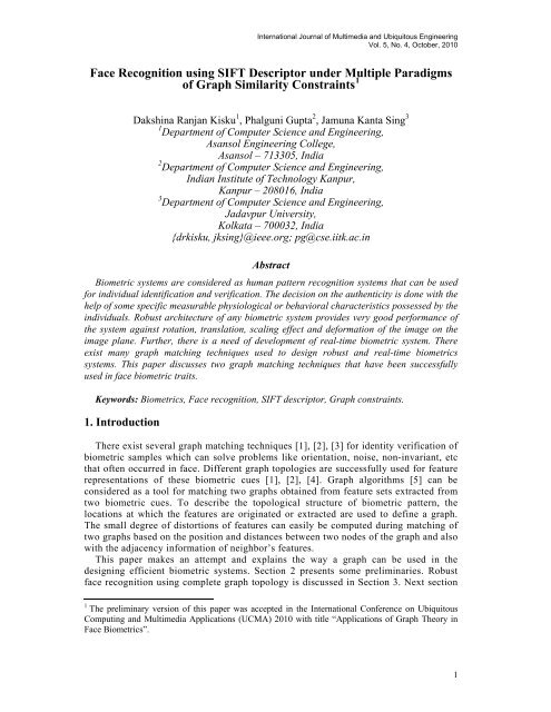
<strong>Face</strong> <strong>Recognition</strong> <strong>using</strong> <strong>SIFT</strong> <strong>Descriptor</strong> <strong>under</strong> <strong>Multi</strong>ple Paradigms<br />
of Graph Similarity Constraints 1<br />
Dakshina Ranjan Kisku 1 , Phalguni Gupta 2 , Jamuna Kanta Sing 3<br />
1 Department of Computer Science and Engineering,<br />
Asansol Engineering College,<br />
Asansol – 713305, India<br />
2 Department of Computer Science and Engineering,<br />
Indian Institute of Technology Kanpur,<br />
Kanpur – 208016, India<br />
3 Department of Computer Science and Engineering,<br />
Jadavpur University,<br />
Kolkata – 700032, India<br />
{drkisku, jksing}@ieee.org; pg@cse.iitk.ac.in<br />
Abstract<br />
Biometric systems are considered as human pattern recognition systems that can be used<br />
for individual identification and verification. The decision on the authenticity is done with the<br />
help of some specific measurable physiological or behavioral characteristics possessed by the<br />
individuals. Robust architecture of any biometric system provides very good performance of<br />
the system against rotation, translation, scaling effect and deformation of the image on the<br />
image plane. Further, there is a need of development of real-time biometric system. There<br />
exist many graph matching techniques used to design robust and real-time biometrics<br />
systems. This paper discusses two graph matching techniques that have been successfully<br />
used in face biometric traits.<br />
Keywords: Biometrics, <strong>Face</strong> recognition, <strong>SIFT</strong> descriptor, Graph constraints.<br />
1. Introduction<br />
There exist several graph matching techniques [1], [2], [3] for identity verification of<br />
biometric samples which can solve problems like orientation, noise, non-invariant, etc<br />
that often occurred in face. Different graph topologies are successfully used for feature<br />
representations of these biometric cues [1], [2], [4]. Graph algorithms [5] can be<br />
considered as a tool for matching two graphs obtained from feature sets extracted from<br />
two biometric cues. To describe the topological structure of biometric pattern, the<br />
locations at which the features are originated or extracted are used to define a graph.<br />
The small degree of distortions of features can easily be computed during matching of<br />
two graphs based on the position and distances between two nodes of the graph and also<br />
with the adjacency information of neighbor’s features.<br />
This paper makes an attempt and explains the way a graph can be used in the<br />
designing efficient biometric systems. Section 2 presents some preliminaries. Robust<br />
face recognition <strong>using</strong> complete graph topology is discussed in Section 3. Next section<br />
1 The preliminary version of this paper was accepted in the International Conference on Ubiquitous<br />
Computing and <strong>Multi</strong>media Applications (UCMA) 2010 with title “Applications of Graph Theory in<br />
<strong>Face</strong> Biometrics”.<br />
1
International Journal of <strong>Multi</strong>media and Ubiquitous Engineering<br />
Vol. 5, No. 4, October, 2010<br />
proposed a probabilistic graph based face recognition. Experimental results are<br />
presented in Section 5 and concluding remarks are made in the last section.<br />
2. Preliminaries<br />
2.1. Scale Invariant Feature Transform (<strong>SIFT</strong>) <strong>Descriptor</strong><br />
To recognize and classify objects efficiently, feature points from objects can be<br />
extracted to make a robust feature descriptor or representation of the objects. David<br />
Lowe has introduced a technique called Scale Invariant Feature Transform (<strong>SIFT</strong>) [7] to<br />
extract features from images. These features are invariant to scale, rotation, partial<br />
illumination and 3D projective transform and they are shown to provide robust<br />
matching across a substantial range of affine distortion, change in 3D viewpoint,<br />
addition of noise and change in illumination. <strong>SIFT</strong> features provide a set of features of<br />
an object that are not affected by occlusion, clutter and unwanted noise in the image. In<br />
addition, <strong>SIFT</strong> features are highly distinctive in nature which have accomplished<br />
correct matching on several pair of feature points with high probability between a large<br />
database and a test sample. Following are the four major filtering steps of computation<br />
used to generate the set of image feature based on <strong>SIFT</strong>.<br />
• Scale-Space Extrema Detection: This filtering approach attempts to identify<br />
image locations and scales that are identifiable from different views. Scale<br />
space and Difference of Gaussian (DoG) functions are used to detect stable<br />
keypoints. Difference of Gaussian is used for identifying key-points in scalespace<br />
and locating scale space extrema by taking difference between two<br />
images, one with scaled by some constant time of the other. To detect the local<br />
maxima and minima, each feature point is compared with its 8 neighbors at the<br />
same scale and in accordance with its 9 neighbors up and down by one scale. If<br />
this value is the minimum or maximum of all these points then this point is an<br />
extrema.<br />
• Keypoints Localization in Laplacian Space: To localize keypoints, few points<br />
after detection of stable keypoint locations that have low contrast or are poorly<br />
localized on an edge are eliminated. This can be achieved by calculating the<br />
Laplacian space. After computing the location of extremum value, if the value<br />
of difference of Gaussian pyramids is less than a threshold value, the point is<br />
excluded. If there is a case of large principle curvature across the edge but a<br />
small curvature in the perpendicular direction in the difference of Gaussian<br />
function, the poor extrema is localized and eliminated.<br />
• Assignment of Orientation: This step aims to assign consistent orientation to<br />
the key-points based on local image characteristics. From the gradient<br />
orientations of sample points, an orientation histogram is formed within a region<br />
around the key-point. Orientation assignment is followed by key-point<br />
descriptor which can be represented relative to this orientation. A 16x16<br />
window is chosen to generate histogram. The orientation histogram has 36 bins<br />
covering 360 degree range of orientations. The gradient magnitude and the<br />
orientation are pre-computed <strong>using</strong> pixel differences. Each sample is weighted<br />
by its gradient magnitude and by a Gaussian-weighted circular window.<br />
2
International Journal of <strong>Multi</strong>media and Ubiquitous Engineering<br />
Vol. 5, No. 4, October, 2010<br />
• Keypoint <strong>Descriptor</strong>: In the last step, the feature descriptors which represent<br />
local shape distortions and illumination changes are computed. After candidate<br />
locations have been found, a detailed fitting is performed to the nearby data for<br />
the location, edge response and peak magnitude. To achieve invariance to image<br />
rotation, a consistent orientation is assigned to each feature point based on local<br />
image properties. The histogram of orientations is formed from the gradient<br />
orientation at all sample points within a circular window of a feature point.<br />
Peaks in this histogram correspond to the dominant directions of each feature<br />
point. For illumination invariance, 8 orientation planes are defined. Finally, the<br />
gradient magnitude and the orientation are smoothened by applying a Gaussian<br />
filter and then are sampled over a 4 x 4 grid with 8 orientation planes.<br />
2.2. Correspondence Graph Definitions<br />
The correspondence graph problem [6] is the problem of finding a match between<br />
two structural descriptions, i.e., a mapping function between elements of two set of<br />
feature points which preserve the compatibilities between feature relations of face<br />
images. Let G1 and G2 be two face graphs given by:<br />
G1 G1<br />
G1<br />
G 2 G 2 G 2<br />
G 1 = { V , E , F }, G2<br />
= { V , E , F }<br />
(1)<br />
where V Gk , E Gk and F Gk represent the set of vertices, edges and <strong>SIFT</strong> features,<br />
respectively, in terms of each feature points associated to the graph, with two face<br />
images k = 1, 2. Let us define the directional correspondence between two feature<br />
points as follows:<br />
2.2.1. Definition 1: Let us assume that the i th (i=1,2,..,N) feature of first face graph<br />
G1 has correspondence to the j th (j =1,2,…,M) feature point on the second face graph<br />
G2 in respect of conditional probability V i G1 → V j G2 , if<br />
G1<br />
G2<br />
G1<br />
G2<br />
p(<br />
Vi = Vj<br />
, Vi<br />
+ 1<br />
= Vj<br />
,..... G1)<br />
−1<br />
≤∈;<br />
∈> 0<br />
(2)<br />
G1 G2<br />
G2<br />
Note that V i → V j does not imply V j → V G1 i . Therefore, to avoid false<br />
correspondences, one-to-one correspondence is defined as the extension of the Equation<br />
(2).<br />
2.2.2. Definition 2: Let the i th feature point of the first face graph G1 has one-to-one<br />
correspondence to the j th feature point on the second face graph G2 in terms of<br />
conditional probability V G1 i ↔V G2 j if<br />
and<br />
G 1 G 2<br />
i<br />
= V<br />
j<br />
G 1) − 1<br />
1<br />
(3)<br />
p ( V<br />
≤∈<br />
3
International Journal of <strong>Multi</strong>media and Ubiquitous Engineering<br />
Vol. 5, No. 4, October, 2010<br />
G 2<br />
for some small ∈ > , ∈ 0<br />
1<br />
0<br />
2<br />
><br />
G 1<br />
i<br />
p ( V<br />
j<br />
= V G 2 ) − 1 ≤∈<br />
(4)<br />
The correspondence graph between G1 and G2 is defined as:<br />
G<br />
G1<br />
G2<br />
G1<br />
G2<br />
G1<br />
G2<br />
G1↔G<br />
2<br />
( V , V , E , E , F , F , C )<br />
G1<br />
↔ G2<br />
= (5)<br />
where G k ⊆ Gk is a sub-graph of the original graph G k , k = 1,2, in which all the nodes<br />
have the one-to-one correspondence to each other such that V G1 i ↔V G2 G 1 G 2<br />
j and C<br />
↔ is<br />
the set of node pairs which have the one-to-one correspondence, given by:<br />
C<br />
G<br />
{ }<br />
1 G<br />
( ,<br />
2 G 1<br />
G<br />
V<br />
2<br />
i<br />
V<br />
j<br />
V<br />
i<br />
↔ V<br />
j<br />
G 1 ↔ G 2 =<br />
)<br />
2<br />
(6)<br />
2.3. Probabilistic Relaxation Graph<br />
In order to interpret a pattern with feature points and graph relaxation topology [10],<br />
each extracted feature can be thought as a node and the relationship between points can<br />
be considered as edge between two nodes. Relaxation graphs are then drawn on the<br />
feature points extracted from the pattern. These relaxations are used for matching and<br />
verification.<br />
Thus, the graph can be represented by G = {V,E,K,ζ}, where V and E denote the set<br />
of nodes and the set of edges, respectively and K and ζ are the sets of attributes<br />
associated with nodes and edges in the graph, respectively. K denotes the set of<br />
keypoint descriptors associated with various nodes and ζ denotes the relationship<br />
between two keypoint descriptors.<br />
Suppose, G R = {V R ,E R ,K R ,ζ R } and G Q = {V Q ,E Q ,K Q ,ζ Q } are two graphs. These two<br />
graphs can be compared to determine whether they are identical or not. If it is found<br />
that |V R | = |V Q | for the given two graphs, the problem is said to be exact graph matching<br />
problem. The problem is to find a one-to-one mapping f: V Q → V R such that (u,v) є E Q<br />
iff (f(u),f(v)) є E R . This mapping f is called an isomorphism and G Q is called isomorphic<br />
to G R . In this case, isomorphism is not possible because identical feature points may not<br />
be present on two different patterns. Hence, it is forced to apply inexact graph matching<br />
problem in the context of probabilistic graph matching where either |V R | < |V Q | or |V R |<br />
> |V Q |. This may occur when the number of points or vertices is different in both the<br />
graphs.<br />
The similarity measure for vertex and edge attributes can be defined as the similarity<br />
measure for nodes v i j<br />
R є V R and v Q є V Q as s v ij = s(v i R , v j i<br />
Q ) where v R є K R є V R and v j Q є<br />
ip<br />
K Q є V Q , and the similarity between edges e R є E R and e jq Q є E Q can be denoted as s e ipjq<br />
= s(e ip R , e jq Q ), where e jp R є ζ R ε E R and e jq Q є ζ Q є E Q .<br />
Now, v j Q would be best probable match for v i R when v j Q maximizes the posteriori<br />
probability of labeling. Thus for the vertex v i R є V R , we are searching the most probable<br />
label or vertex v -i R = v j Q є V Q in the graph. Hence, it can be stated as<br />
4
International Journal of <strong>Multi</strong>media and Ubiquitous Engineering<br />
Vol. 5, No. 4, October, 2010<br />
v<br />
i<br />
R<br />
Q<br />
= arg max P(<br />
ψ | K , ς , K , ς )<br />
(7)<br />
j , v<br />
Q<br />
∈V<br />
Q<br />
v<br />
i<br />
j<br />
R<br />
R<br />
Q<br />
Q<br />
For efficient searching of matching probabilities from the query sample, we use<br />
v<br />
relaxation technique which simplifies the solution of matching problem. Let P denote<br />
ij<br />
the matching probability for vertices v i j<br />
R є V R and v Q є V Q . Now, by reformulating<br />
Equation (7) one gets<br />
i<br />
v<br />
v R<br />
= arg max Pij<br />
j , vQ<br />
∈V<br />
j Q<br />
(8)<br />
Equation (8) is considered as an iterative relaxation algorithm for searching the best<br />
v<br />
labels for v i Pij<br />
R. This can be achieved by assigning prior probability proportional<br />
v v i j<br />
v<br />
s<br />
ij<br />
= s ( k<br />
R<br />
, kQ<br />
)<br />
P<br />
ij<br />
to<br />
. The following iterative relaxation rule can be used to define ;<br />
Pˆ<br />
v<br />
ij<br />
=<br />
j , v<br />
∑<br />
j<br />
Q<br />
P<br />
v<br />
ij<br />
∈ V Q<br />
. Q<br />
P<br />
v<br />
ij<br />
ij<br />
. Q<br />
ij<br />
(9)<br />
where, Q ij is given by<br />
∏<br />
v i ∈V<br />
R<br />
∑<br />
v<br />
e<br />
Q = P<br />
s . P<br />
ij<br />
ij<br />
v j ∈V<br />
Q<br />
ij<br />
v<br />
ij<br />
(10)<br />
In Equation (10), Q ij conveys the support of the neighboring vertices and represents<br />
the posteriori probability. The relaxation cycles are repeated until the difference<br />
between prior probability P and posteriori probabilities Pˆ becomes smaller than<br />
v<br />
ij<br />
certain threshold Φ . When it is achieved then it is assumed that the relaxation process is<br />
stable.<br />
3. <strong>Face</strong> <strong>Recognition</strong> <strong>using</strong> Complete Graph Topology<br />
The proposed face recognition technique has been designed by <strong>using</strong> the complete<br />
graph topology which makes use of invariant <strong>SIFT</strong> features. The technique is developed<br />
with the three graph matching constraints, namely Gallery Image based Match<br />
Constraint [6], Reduced Point based Match Constraint [6] and Regular Grid based<br />
Match Constraint [6]. Initially the face image is normalized by <strong>using</strong> histogram<br />
equalization. The rotation, scale and partial illumination invariant <strong>SIFT</strong> features are<br />
then extracted from the normalized face images. Finally, the graph-based topology is<br />
applied for matching two face images.<br />
v<br />
ij<br />
v<br />
Pˆ<br />
ij<br />
5
International Journal of <strong>Multi</strong>media and Ubiquitous Engineering<br />
Vol. 5, No. 4, October, 2010<br />
3.1 Gallery Image based Match Constraint<br />
It is assumed that matching points can be found around similar positions i.e., fiducial<br />
points on the face image. To eliminate false matches a minimum Euclidean distance<br />
measure is applied. It may be possible that more than one point in the first image<br />
correspond to the same point in the second image. Let us consider, X 1 ,X 2 ,…,X N are the<br />
interest points found in the first image and Y 1 ,Y 2 ,…,Y M are the interest points found in<br />
the second image. Whenever N ≤ M, many interest points from the second image are<br />
discarded, while if N ≥ M, many repetitions of the same point would be occurred as<br />
corresponding points in the second image. In both cases, one interest point of the<br />
second image may correspond to several points in the first image. After computing all<br />
the distances, only the point with the minimum distance from the corresponding point in<br />
the second image is paired (It has been illustrated in Fig. 1 and Fig. 2).<br />
6.9<br />
X 1<br />
Y 1<br />
Y 9<br />
X 2<br />
7.2<br />
7.6<br />
X 3<br />
X i<br />
X<br />
9.7<br />
10.9<br />
Y i<br />
First <strong>Face</strong> Image<br />
Second <strong>Face</strong> Image<br />
Figure 1. The Corresponding Points of Image 1 are Mapped into Image 2 <strong>using</strong><br />
the Minimum Euclidean Distance Measure<br />
50<br />
100<br />
150<br />
200<br />
50 100 150 200 250 300 350 400<br />
Figure 2. All Feature Points and their Matches for a Pair of Images, based on<br />
Euclidean Distance Measure<br />
6
International Journal of <strong>Multi</strong>media and Ubiquitous Engineering<br />
Vol. 5, No. 4, October, 2010<br />
The distances are computed based on the Hausdorff distance between two images.<br />
The dissimilarity scores are computed between all pairs of nodes of two face images<br />
after constructing the complete graph for each face image.<br />
Suppose, F gallery and F probe , are two images representing the gallery and probe image,<br />
respectively and I is the compact information composed of all the four types of<br />
information generated by the <strong>SIFT</strong> descriptor. Then we have,<br />
F<br />
F<br />
gallery<br />
gallery<br />
gallery<br />
gallery<br />
I( Fgallery)<br />
= { X ( fi<br />
), K ( fi<br />
), S ( fi<br />
), O ( fi<br />
)}<br />
Fprobe Fprobe Fprobe<br />
probey<br />
I( Fprobe)<br />
= { X ( f<br />
j),<br />
K ( f<br />
j<br />
), S ( f<br />
j<br />
), O ( f<br />
j<br />
)}<br />
where i = 1,2,…….,N; j = 1,2,………,M;<br />
The dissimilarity scores D GIBMC V(F gallery , F probe ) and D GIBMC E(F gallery , F probe ) are<br />
computed for both the vertexes and the edges as:<br />
F<br />
F<br />
F<br />
D<br />
GIBMC<br />
V<br />
( F<br />
gallery<br />
, F<br />
probe<br />
) = min { min ( d ( I<br />
i<br />
( Fgallery<br />
), I<br />
j<br />
( Fprobe<br />
))} (11)<br />
i=<br />
1,2,.., N<br />
j=<br />
1,2,..., M<br />
Δ<br />
GIBMC<br />
V<br />
T<br />
1 GIBMC<br />
t<br />
( F<br />
gallery<br />
, F<br />
probe<br />
) = ∑ D V ( F<br />
gallery<br />
, F<br />
probe<br />
)<br />
(12)<br />
T<br />
t = 1<br />
where T is the total number of all is minimum distances. To find the correspondences<br />
between two graphs in terms of edge information, let us take E 1 (N) and E 2 (N) are the<br />
number of edges in the two face graphs respectively and the number of nodes for two<br />
images are same. After finding the corresponding points between the feature points of<br />
the first and the second image, we construct complete graph for each face image. We<br />
try to find out the correspondences and compute the dissimilarity scores for a pair of<br />
edges. If nodes a,a’є N gallery and b,b’є N probe belong to gallery and probe images,<br />
respectively, then (a,a’) є E 1 (N) and (b,b’) є E 2 (N) would be a pair of edges for the<br />
gallery image and the probe image, respectively and score is given by<br />
D<br />
( F , F ) d(<br />
I ( F ( a,<br />
a′<br />
)), I ( F ( b,<br />
b )))<br />
= (13)<br />
GIBMC<br />
E<br />
′<br />
gallery probe<br />
i gallery<br />
j probe<br />
Δ<br />
GIBMC<br />
E<br />
e = 1<br />
where i,j = 1,2,…,N;<br />
E<br />
1 GIBMC<br />
e<br />
( Fgallery<br />
, Fprobe<br />
) = ∑ D E ( Fgallery<br />
, Fprobe<br />
)<br />
(14)<br />
E<br />
where d(I i (F gallery (a,a’))I j (F probe (b,b’))) is the distance between a pair of edges and<br />
D GIBMC E(F gallery , F probe ) is the average distance of all pairs of edges.<br />
3.2. Reduced Point based Match Constraint<br />
7
International Journal of <strong>Multi</strong>media and Ubiquitous Engineering<br />
Vol. 5, No. 4, October, 2010<br />
After eliminating the points that do not satisfy the gallery image point based match<br />
constraints, there can still be some false matches. Usually, the false matches are due to<br />
multiple assignments. These false matches can be eliminated by the help of an example<br />
shown in Fig. 3. Note that more than one point (e.g, X2, X3 and XN) are assigned to a<br />
single point (e.g. Y9) in the other image.<br />
These false matches can be eliminated by applying another constraint, namely the<br />
reduced point based match constraint which guarantees that each assignment from an<br />
image X to another imag e Y has a corresponding assignment from image Y to<br />
image X . With this constraint, the false matches due to multiple assignments are<br />
eliminated by choosing the match with the minimum distance. The false matches due to<br />
one way assignments are eliminated by removing the links which do not have any<br />
corresponding assignment from the other side. Examples showing the matches before<br />
and after applying the reduced point based match constraints are given in Fig. 4.<br />
X 2<br />
7.6<br />
X 3<br />
7.2<br />
Y 9<br />
X N<br />
9.7<br />
First <strong>Face</strong> Image<br />
Second <strong>Face</strong> Image<br />
Figure 3. An Example of <strong>Multi</strong>ple Assignments of points of First Image to a<br />
Single Point of Second Image<br />
In this graph matching strategy, the same approach is followed which is described in<br />
the gallery image based match constraint. False matches, due to multiple assignments,<br />
are removed by choosing the match with the minimum distance between two face<br />
images. The dissimilarity scores on reduced points between two face images for nodes<br />
and edges are computed in the same way as for the gallery based constraint.<br />
50<br />
50<br />
100<br />
100<br />
150<br />
150<br />
200<br />
200<br />
50 100 150 200 250 300 350 400<br />
50 100 150 200 250 300 350 400<br />
4(a)<br />
4(b)<br />
8
International Journal of <strong>Multi</strong>media and Ubiquitous Engineering<br />
Vol. 5, No. 4, October, 2010<br />
Figure 4. An Example of Reduced Point based Match Constraint. (a) All<br />
Matches Computed from the Left to the Right Image. (b) The Resulting<br />
Complete Graphs with a Few Numbers of False Matches<br />
3.3. Regular Grid based Match Constraint<br />
The graph matching technique presented in this section has been developed with the<br />
concept of matching of corresponding sub-graphs for a pair of face images. First the<br />
face image is divided into sub-images, <strong>using</strong> a regular grid with overlapping regions.<br />
The matching between a pair of face images is performed by comparing sub-images and<br />
computing distances between all pairs of corresponding sub-image graphs in a pair of<br />
face images and finally averaging the dissimilarity scores for a pair of sub-images.<br />
From an experimental evaluation, we have considered sub-images of dimensions 1/5 of<br />
width and 1/5 of height as a good compromise between localization accuracy and<br />
robustness to registration errors on a face image. The overlapping is set to 30%.<br />
When we compare a pair of corresponding sub-image graphs for a pair of face<br />
images, we eliminate false match pair assignments by choosing a minimum distance<br />
assignment between a pair of points. Let us consider face image is divided into G<br />
number of equal regions and for each pair of sub-regions invariant <strong>SIFT</strong> features are<br />
selected. We construct sub-graphs on a pair of corresponding sub-regions. While a<br />
direct comparison is made between a pair vertices and a pair of edges for a pair of subregions,<br />
the dissimilarity scores are computed. These dissimilarity scores represent<br />
distance between corresponding sub-graphs. The dissimilarity scores D RGBMC V(F gallery ,<br />
F probe ) are computed for a pair of vertices as:<br />
D<br />
RGBMC<br />
V<br />
( F<br />
gallery<br />
, F<br />
probe<br />
) =<br />
min { min ( d(<br />
I ( F<br />
i=<br />
1,2,.., N<br />
j=<br />
1,2,..., M<br />
i<br />
gallery<br />
), I<br />
j<br />
( F<br />
probe<br />
))}<br />
(15)<br />
Δ<br />
RGBMC<br />
V<br />
k 1 RGBMC<br />
t′<br />
( Fgallery,<br />
Fprobe)<br />
= D V ( Fgallery,<br />
Fprobe)<br />
(16)<br />
T′<br />
T<br />
∑ ′<br />
t′=<br />
1<br />
where T′ is the total number of minimum distances between a pair of face sub-graphs<br />
and Δ RGBMC V(F gallery , F probe ) k (where k = 1,2,3,…,G ) is the mean distance between a pair<br />
of face sub-graphs in terms of composed invariant values which are associated to each<br />
vertex.<br />
Similarly, to find the dissimilarity scores D RGBMC E(F gallery , F probe ) for a pair of edges,<br />
let us take E 1 ′ (N) and E 2 ′ (N) are the number of edges for a pair of face sub-graphs,<br />
respectively. If N vertices in face sub-graph of gallery face are paired with the same<br />
number of vertices in face sub-graph of probe image, respectively, then (c,c’) є E’ 1 (N)<br />
and (d,d’) є E’ 2 (N) would be a pair of edges for a pair of face sub-graphs.<br />
D<br />
RGBMC<br />
E ( F , F ) d(<br />
I ( F ( c,<br />
c′<br />
gallery probe<br />
i gallery<br />
)), I<br />
j<br />
( Fprobe<br />
( d,<br />
d ′<br />
= (17)<br />
)))<br />
where i= 1,2,3,…N and j = 1,23,...,N;<br />
9
International Journal of <strong>Multi</strong>media and Ubiquitous Engineering<br />
Vol. 5, No. 4, October, 2010<br />
Δ<br />
RGBMC<br />
E<br />
E<br />
k 1 RGBMC<br />
e<br />
( Fgallery<br />
, F<br />
probe<br />
) = ∑ D E ( Fgallery<br />
, F<br />
probe<br />
)<br />
(18)<br />
E<br />
e = 1<br />
where E is the total number of minimum distances between a pair of face sub-graphs<br />
and Δ RGBMC E(F gallery , F probe ) k (where k = 1,2,3,…,G ) is the mean distance between a pair<br />
of face sub-graphs for a pair of edges. By adding mean distances Δ RGBMC V(F gallery ,<br />
F probe ) k and Δ RGBMC E(F gallery , F probe ) k for vertices and edges respectively and dividing by<br />
2, we get a mean dissimilarity value D RGBMC (I gallery , I probe ) for a pair of face sub-graphs.<br />
Finally, the weighted matching score Δ RGBMC (I gallery , I probe ) is computed as the mean<br />
distance between a pair of face images. Weight assignment to each feature is done by<br />
Gaussian Empirical Rule.<br />
3.4. Weighting the Score Reliability<br />
The quality of the features has a significant impact on the performance of any<br />
learning based recognition algorithm. The way to improve the quality of features has<br />
been one of the critical issues concerned with the instance-based learning. Various<br />
approaches have been proposed in the past to address this issue. These approaches can<br />
be mainly divided into feature selection and feature weighting.<br />
This work proposes a feature weighting method that is based on the Gaussian<br />
empirical rule. In this method, the relevance of a feature is determined by assigning a<br />
weight <strong>using</strong> the Gaussian empirical rule. The rationale behind this idea is that a<br />
relevant feature should have strong impact on classification. One advantage of <strong>using</strong> the<br />
Gaussian empirical rule for feature weighting is its rich expressiveness in representing<br />
hypotheses. In order to determine the weighted distance between two graphs, the<br />
weights can be assigned by applying the Gaussian empirical rule which satisfies the<br />
properties describe in [6].<br />
Before generating the weighted dissimilarity scores, for each pair of face images, the<br />
mean and standard deviation are computed for a set of nodes and for a set of edges on<br />
the face graph.<br />
If the node and edge values lie within one, two and three times of the standard<br />
deviation of the mean, they are multiplied by 0.075 or 0.05 or 0.025 respectively. These<br />
values have been determined by a through testing on the BANCA database.<br />
3.5. Fusion of Matching Scores<br />
Since Regular Grid based and Reduced Point Based match constraints show increase<br />
in accuracy, therefore we fuse these two match constraints <strong>using</strong> sum rule [15] in terms<br />
of matching scores obtained from these two methods. Prior to fusion of these two<br />
k<br />
matchers, scores are normalized by min-max normalization rule [15]. Let n i<br />
normalized score for matcher k (k = 1,2,3, …, K; K be the number of matchers) and i (i<br />
= 1,2,3,…,I) is the user. The fused score F i for user i can be given by<br />
F<br />
i<br />
=<br />
K<br />
∑<br />
k = 1<br />
n<br />
k<br />
i<br />
, ∀ i<br />
(19)<br />
10
International Journal of <strong>Multi</strong>media and Ubiquitous Engineering<br />
Vol. 5, No. 4, October, 2010<br />
Therefore, the match scores obtained from RGBMC and RPBMC methods can be fused<br />
by <strong>using</strong> the Equation (19) and the score F i for user i can be given by<br />
F<br />
( RGBMC<br />
i<br />
+ RPBMC<br />
)<br />
=<br />
n<br />
RGBMC<br />
i<br />
+<br />
n<br />
RPBMC<br />
i<br />
, ∀ i<br />
(20)<br />
4. <strong>Face</strong> <strong>Recognition</strong> <strong>using</strong> Probabilistic Relaxation Graph<br />
This section proposes a novel local feature based face recognition technique which<br />
makes use of dynamic (mouth) and static (eyes, nose) salient features of face obtained<br />
through <strong>SIFT</strong> operator [7]. Differences in facial expression, head pose, illumination,<br />
and partly occlusion may result to variations of facial characteristics and attributes. To<br />
capture the face variations, face characteristics of dynamic and static parts are further<br />
represented by incorporating repetitive probabilistic graph relaxations drawn on <strong>SIFT</strong><br />
features extracted from localized mouth, eyes and nose facial parts.<br />
To localize the major facial features such as eyes, mouth and nose, positions are<br />
automatically located by applying the technique in [8], [9]. A circular region of interest<br />
(ROI) centered at each extracted facial landmark location is considered to determine the<br />
<strong>SIFT</strong> features of the landmark. The face recognition system can use <strong>SIFT</strong> descriptor for<br />
extraction of invariant features from each facial landmark, namely, eyes, mouth and<br />
nose shown in Fig. 5.<br />
50<br />
50<br />
100<br />
100<br />
150<br />
150<br />
200<br />
200<br />
50 100 150 200<br />
50 100 150 200<br />
4.1 Fusion of Matching Scores<br />
Figure 5. <strong>SIFT</strong> Features on Facial Landmarks<br />
The Dempster-Shafer decision theory [11] which is applied to combine the matching<br />
scores obtained from individual landmark is based on combining the evidences obtained<br />
from different sources to compute the probability of an event. This is obtained by<br />
combining three elements: the basic probability assignment function (bpa), the belief<br />
function (bf) and the plausibility function (pf).<br />
left−eye right−eye nose<br />
mouth<br />
Let Γ , Γ , Γ and Γ be the individual matching scores obtained<br />
from the four different matching of salient facial landmarks. In order to obtain the<br />
combine matching score from the four salient landmarks pairs, Dempster combination<br />
rule has been applied. First, we combine the matching scores obtained from the pairs of<br />
11
International Journal of <strong>Multi</strong>media and Ubiquitous Engineering<br />
Vol. 5, No. 4, October, 2010<br />
left-eye and nose landmark features and then the matching scores obtained from the<br />
pairs of right-eye and mouth landmark features are combined. Finally, the matching<br />
left−eye<br />
scores determined from the first and second processes are fused. Also, let m(<br />
Γ ) ,<br />
right−eye<br />
nose<br />
mouth<br />
m(<br />
Γ ) , m(<br />
Γ ) and m(<br />
Γ ) be the bpa functions for the Belief measures<br />
left−eye<br />
right−eye<br />
nose<br />
mouth<br />
Bel(<br />
Γ ) , Bel(<br />
Γ ) , Bel( Γ ) and Bel(<br />
Γ ) for the four classifiers,<br />
left−eye<br />
right−eye<br />
respectively. Then the Belief probability assignments (bpa) m(<br />
Γ ) , m(<br />
Γ ) ,<br />
nose<br />
mouth<br />
m(<br />
Γ ) and m(<br />
Γ ) can be combined together to obtained a Belief committed to a<br />
matching score set C ∈ Θ <strong>using</strong> orthogonal sum rule [11].<br />
The final decision of user acceptance and rejection can be established by applying<br />
threshold to the final match score.<br />
5. Experimental Results<br />
To verify the efficacy and robustness of graph matching techniques discussed in the<br />
paper, three face databases such as BANCA [12], ORL [13] and IIT Kanpur [14]<br />
databases are used for evaluation. This paper describes two different graph based<br />
matching techniques, namely, complete graph based match constraints and probabilistic<br />
graph based matching technique.<br />
5.1 Experimental Results Determined from Complete Graph based Matching<br />
The proposed complete graph based matching technique for face recognition has<br />
been used the BANCA database for testing. BANCA face database [12] consists of<br />
4160 face images obtained from 208 subjects of 4 different languages with 52 subjects<br />
(26 males and 26 females) for each language and each subject having 20 face images.<br />
Each language-gender specific population of 26 subjects is divided itself into two<br />
groups and each having 13 subjects each. The two groups are denoted as g1 and g2.<br />
<strong>Face</strong> images of each subject have recorded in controlled, degraded and adverse<br />
conditions with over 12 different sessions spanning three months.<br />
<strong>Face</strong> images in different conditions are shown in Fig. 6. The face images are<br />
presented with changes in pose, in illumination and in facial expression. The BANCA<br />
face database considered as one of the complex databases for experiment. There are<br />
seven different protocols are constructed for evaluation. Such as Matched Controlled<br />
(MC), Matched Degraded (MD), Matched Adverse (MA), Unmatched Degraded (UD),<br />
Unmatched Adverse (UA), Pooled Test (PT) and Grand Test (GT). For this experiment,<br />
the Matched Controlled (MC) protocol is followed where the images from the first<br />
session are used for training and second, third, and fourth sessions are used for testing<br />
and generating client and impostor scores. Three graph matching constraints which are<br />
Gallery Image based Match Constraint (GIBMC), Reduced Point based Match<br />
Constraint (RPBMC) and Regular Grid based Match Constraint (RGBMC) have been<br />
tested with BANCA face database. The test images are divided into two groups, G1 and<br />
G2, of 26 subjects each.<br />
12
International Journal of <strong>Multi</strong>media and Ubiquitous Engineering<br />
Vol. 5, No. 4, October, 2010<br />
Figure 6. <strong>Face</strong> Images from BANCA Database in different Scenarios. First Row:<br />
Controlled, Second Row: Degraded, Third Row: Adverse.<br />
The error rates [14] have been computed <strong>using</strong> the following procedure:<br />
• For getting scores of G1, perform the experiment on G1.<br />
• Perform the experiment on G2, to get scores of G2.<br />
• Compute the ROC curve <strong>using</strong> G1 scores; determine the Prior Equal Error<br />
Rate and the corresponding client-specific threshold for each subject or each<br />
individual from several instances.<br />
• Use the threshold T G1 to compute False Acceptance Rate (FAR G2 (T G1 )) and<br />
False Rejection Rate (FRR G2 (T G1 )) on the G2 scores. The threshold is clientspecific<br />
i.e, is computed specifically for each individual from the several<br />
instances of his/her images.<br />
• Compute the weighted Error Rate (WER(R)) on G2:<br />
WER<br />
( R ) =<br />
FRR<br />
G 2<br />
( T<br />
G 1<br />
) + R × FAR<br />
1 + R<br />
G 2<br />
( T<br />
G 1<br />
)<br />
(20)<br />
for R = 0.1, 1 and 10 (R is defined as the cost ratio for three different operating points,<br />
namely, R = 0.1, R = 1 and R = 10). WER(R) is computed on G1 by a dual approach<br />
where the parameter R indicates the cost ratio between false acceptance and false<br />
rejection.<br />
Prior Equal Error Rates for G1 and G2 are presented in Table 1 and Table 2 showing<br />
WER for three different values of R.<br />
13
International Journal of <strong>Multi</strong>media and Ubiquitous Engineering<br />
Vol. 5, No. 4, October, 2010<br />
Table 1. Prior EER on G1 and G2 for the Four Methods: ‘GIBMC’ Stands for<br />
Gallery Image Based Match Constraint, ‘RPBMC’ Stands for Reduced Point<br />
Based Match Constraint, ‘RGBMC’ Stands for Regular Grid Based Match<br />
Constraint and the Fusion of RPBMC and RGBMC<br />
Methods GIBMC (%) RPBMC (%) RGBMC (%) Fusion (%)<br />
EER ↓<br />
Prior EER on G1 10.13 6.66 4.6 2.02<br />
Prior EER on G2 6.46 1.92 2.52 1.56<br />
Average 8.29 4.29 3.56 1.79<br />
From Table 2 it can be seen that WER for Reduced Point based Match Constraint<br />
determined on G2 is very low while it is compared with other two match constraints.<br />
On the other hand, WER on G1 determined with Regular Grid based Match Constraint<br />
shows low as it is compared with GIBMC and RPBMC. For G1, Regular Grid based<br />
Match Constraint outperforms others and for G2, Reduced Point based Match<br />
Constraint performance is better than other two techniques. Therefore, the significant<br />
number of features that forming better matched pair of <strong>SIFT</strong> feature points can be<br />
efficiently used in Reduced Point based Match Constraint (RPBMC) and Regular Grid<br />
based Match Constraint (RGBMC). Further RGBMC uses grids on face image which<br />
are formed by dividing the image into 5×5 equal regions with the consideration of 30%<br />
overlapping of sub-region boundaries. However, the fusion of RGBMC and RPBMC<br />
methods outperforms the RGBMC and RPBMC. Fusion method achieves 1.79% EER.<br />
Table 2. WER for the Four Different Matching Techniques: ‘GIBMC’ Stands<br />
for Gallery Image Based Match Constraint, ‘RPBMC’ Stands for Reduced<br />
Point Based Match Constraint, ‘RGBMC’ Stands for Regular Grid Based Match<br />
Constraint and Fusion Method<br />
Methods <br />
WER ↓<br />
WER (R = 0.1) on G1<br />
WER (R = 0.1) on G2<br />
WER (R = 1) on G1<br />
WER (R = 1) on G2<br />
WER (R = 10) on G1<br />
WER (R = 10) on G2<br />
GIBMC (%) RPBMC (%) RGBMC (%) Fusion (%)<br />
10.24<br />
6.83<br />
10.13<br />
6.46<br />
10.02<br />
6.09<br />
7.09<br />
2.24<br />
6.66<br />
1.92<br />
6.24<br />
1.61<br />
4.07<br />
3.01<br />
4.6<br />
2.52<br />
4.12<br />
2.02<br />
3.01<br />
2.95<br />
3.34<br />
1.09<br />
3.76<br />
1.21<br />
5.2 Experimental Results Determined from Probabilistic Graph Matching<br />
The IITK face database [14] consists of 1200 face images with four images per<br />
person (300X4). These images are captured <strong>under</strong> control environment with ±20-30<br />
degree changes of head pose and with at most uniform lighting and illumination<br />
conditions and with consistent facial expressions. For the face matching, all probe<br />
images are matched against all target images. From the ROC curve in Fig. 7 it has been<br />
14
International Journal of <strong>Multi</strong>media and Ubiquitous Engineering<br />
Vol. 5, No. 4, October, 2010<br />
observed that the recognition accuracy is 93.63%, with the false accept rate (FAR) of<br />
5.82%.<br />
100<br />
ROC Curves Determined from ORL and IITK <strong>Face</strong> Database<br />
90<br />
<br />
80<br />
70<br />
60<br />
50<br />
40<br />
30<br />
ROC curve for ORL face database<br />
ROC curve for IITK face database<br />
20<br />
10 0 10 1 10 2<br />
<br />
Figure 7. ROC Curves<br />
The ORL face database [13] consists of 400 images taken from 40 subjects. Out of<br />
these 400 images, 200 face images are considered for experiment. It has been observed<br />
that there exist changes in orientation in images which lying between -20 0 and 30 0 . The<br />
face images are found to have the variations in pose and facial expression (smile/not<br />
smile, open/closed eyes). The original resolution of the images is 92 x 112 pixels.<br />
However, for the experiment, the resolution is set to 120×160 pixels. From the ROC<br />
curve in Fig. 7 it has been observed that the recognition accuracy for the ORL database<br />
is 97.33%, yielding 2.14% FAR. The relative accuracy of the matching strategy for<br />
ORL database increases of about 3% over the IITK database.<br />
6. Conclusion<br />
In this paper, two face recognition systems have presented <strong>using</strong> complete graph<br />
topology and probabilistic relaxation graph matching respectively. The proposed<br />
systems exhibit robustness towards recognize the users. The results of the Reduced<br />
Point based Match Constraint and the Regular Grid based Match constraint show the<br />
capability of the system to cope for illumination changes and occlusions occurring in<br />
the database or the query face image. Moreover the fusion of these two method exhibits<br />
robust performance which outperforms these two methods. From the second face<br />
recognition it has been determined that when the face matching accomplishes with the<br />
whole face region, the global features (whole face) are easy to capture and they are<br />
generally less discriminative than localized features. In the face recognition method,<br />
local facial landmarks are considered for further processing. The optimal face<br />
15
International Journal of <strong>Multi</strong>media and Ubiquitous Engineering<br />
Vol. 5, No. 4, October, 2010<br />
representation <strong>using</strong> graph relaxation drawn on local landmarks allows matching the<br />
localized facial features efficiently by searching the correspondence of keypoints <strong>using</strong><br />
iterative relaxation.<br />
References<br />
[1] L. Wiskott, J. M. Fellous, N. Kruger, C. Von der Malsburg, “<strong>Face</strong> <strong>Recognition</strong> by Elastic Bunch Graph<br />
Matching”, IEEE Transactions on Pattern Analysis and Machine Intelligence, Vol. 19, No. 7, 1997, pp. 775 – 79.<br />
[2] E. Fazi-Ersi, J. S. Zelek, J. K. Tsotsos, “Robust <strong>Face</strong> <strong>Recognition</strong> through Local Graph Matching”, Journal of<br />
Computers, Vol. 2, No. 5, 2007, pp. 31 – 37.<br />
[3] J. Liu, Z-Q. Liu, “EBGM with Fuzzy Fusion on <strong>Face</strong>”, Advances in Artificial Intelligence, LNCS, Vol. 3809,<br />
2005, pp. 498 – 509.<br />
[4] S. Z. Li, A. K. Jain, (Eds.), Handbook of <strong>Face</strong> <strong>Recognition</strong>, Springer, 2005.<br />
[5] D. Conte, P. Foggia, C. Sansone, M. Vente, “Graph Matching Applications in Pattern <strong>Recognition</strong> and Image<br />
Processing”, International Conference on Image Processing, 2003.<br />
[6] D. R. Kisku, A. Rattani, E. Grosso, M. Tistarelli, “<strong>Face</strong> Identification by <strong>SIFT</strong>-based Complete Graph<br />
Topology. In 5th IEEE International Workshop on Automatic Identification Advanced Technologies, 2007, pp.<br />
63—68<br />
[7] D. G. Lowe, “Object <strong>Recognition</strong> from Local Scale Invariant Features”, International Conference on Computer<br />
Vision, 1999, pp. 1150–1157.<br />
[8] N. Gourier, D. H. James, L. Crowley, “Estimating <strong>Face</strong> Orientation from Robust Detection of Salient Facial<br />
Structures”, FG Net Workshop on Visual Observation of Deictic Gestures, 2004.<br />
[9] F. Smeraldi, N. Capdevielle, J. Bigün, “Facial Features Detection by Saccadic Exploration of the Gabor<br />
Decomposition and Support Vector Machines”, 11th Scandinavian Conference on Image Analysis, 1999, pp. 39 –<br />
44.<br />
[10] D. R. Kisku, H. Mehrotra, P. Gupta, J. K. Sing, “Probabilistic Graph-based Feature Fusion and Score Fusion<br />
<strong>using</strong> <strong>SIFT</strong> Features for <strong>Face</strong> and Ear Biometrics”, SPIE International Symposium on Optics and Photonics,<br />
Vol. 7443, 744306, 2009.<br />
[11] M. Bauer, “Approximation Algorithms and Decision-making in the Dempster-Shafer Theory of Evidence—<br />
An Empirical Study”, International Journal of Approximate Reasoning, Vol. 17, 1997, pp. 217–237.<br />
[12] E. Bailly-Baillire, S. Bengio, F. Bimbot, M. Hamouz, J. Kitler, J. Marithoz, J. Matas, K. Messer, V. Popovici,<br />
F. Pore, B. Ruiz, J. P. Thiran, “The BANCA database and evaluation protocol”, International Conference on Audio<br />
– and Video-Based Biometric Person Authentication, 2003, pp. 625 – 638.<br />
[13] F. Samaria, A. Harter, “Parameterization of a Stochastic Model for Human <strong>Face</strong> Identification”, IEEE<br />
Workshop on Applications of Computer Vision, 1994.<br />
[14] D. R. Kisku, A. Rattani, M. Tistarelli, P. Gupta, “Graph Application on <strong>Face</strong> for Personal Authentication<br />
and <strong>Recognition</strong>”, 10th IEEE International Conference on Control, Automation, Robotics and Vision, 2008, pp.<br />
1150—1155.<br />
[15] R. Snelick, U. Uludag, A. Mink, M. Indovina, A. Jain, "Large Scale Evaluation of <strong>Multi</strong>modal Biometric<br />
Authentication Using State-of-the-Art Systems", IEEE Transactions on Pattern Analysis and Machine<br />
Intelligence , Vol. 27, No. 3, 2005, pp. 450 – 455.<br />
16
International Journal of <strong>Multi</strong>media and Ubiquitous Engineering<br />
Vol. 5, No. 4, October, 2010<br />
Authors<br />
Mr. Dakshina Ranjan Kisku received the B.E. and M.E. degrees<br />
in Computer Science and Engineering from Jadavpur University,<br />
India in 2001 and 2003 respectively. Currently he is an Assistant<br />
Professor in the Department of Computer Science & Engineering,<br />
Asansol Engineering College, Asansol, India and also pursuing<br />
Ph.D. in Engineering at Jadavpur University, India. He works in<br />
the field of biometrics, computer vision and image analysis. He<br />
was a researcher in the Computer Vision Laboratory, University of<br />
Sassari, Italy in 2006. He is an author of 5 book chapters and he<br />
has published more than 35 papers in International Journals and<br />
International Conferences. He has vast experience in teaching in<br />
different engineering colleges. Prior to joining Asansol<br />
Engineering College in June 2010, he was a Senior Lecturer and Project Associate at<br />
Dr. B. C. Roy Engineering College, India and at IIT Kanpur, India in 2008 and 2005,<br />
respectively.<br />
Dr. Phalguni Gupta received the Doctoral degree from Indian<br />
Institute of Technology Kharagpur, India in 1986. Currently he is<br />
a Professor in the Department of Computer Science &<br />
Engineering, Indian Institute of Technology Kanpur (IITK),<br />
Kanpur, India. He works in the field of biometrics, data<br />
structures, sequential algorithms, parallel algorithms, image<br />
processing. He is an author of 2 books and 12 book chapters. He<br />
has published more than 200 papers in International Journals and<br />
International Conferences. He is responsible for several research<br />
projects in the area of Biometric Systems, Image Processing, Graph Theory and<br />
Network Flow. Prior to joining IITK in 1987, he worked in Space Applications Centre<br />
Ahmedabad, Indian Space Research Organization, India.<br />
Dr. Jamuna Kanta Sing received his B.E. degree in<br />
Computer Science & Engineering from Jadavpur University in<br />
1992, M.Tech. degree in Computer & Information Technology<br />
from Indian Institute of Technology (IIT) Kharagpur in 1993 and<br />
Ph.D. (Engineering) degree from Jadavpur University in 2006.<br />
Dr. Sing has been a faculty member of the Department of<br />
Computer Science & Engineering, Jadavpur University since<br />
March 1997. He has done his Post Doctoral research works as a<br />
BOYSCAST Fellow of the Department of Science &<br />
Technology, Govt. of India, at the University of Pennsylvania<br />
and the University of Iowa during 2006. He is a member of the IEEE, USA. His<br />
research interest includes face recognition/detection, medical image processing, and<br />
pattern recognition.<br />
17
International Journal of <strong>Multi</strong>media and Ubiquitous Engineering<br />
Vol. 5, No. 4, October, 2010<br />
18