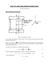
Problem 1:

ENGRD 221 – Prof. N. Zabaras 9/03/07
Recitation Handout 2
ENRGD 221: Engineering Thermodynamics – Prof. Zabaras
Topics covered in class: Chapters 2 and 3
RETRIEVING THERMODYNAMIC PROPERTIES
The emphasis in this class is to retrieve thermodynamic properties using tables
commonly available for pure simple compressible substances.
Page 815 of your text gives a list of all tables for appropriate quantities in S.I. units.
Tables A-2 through A-6 (pages 817-826 in the text) give the properties of water – These
tables are frequently referred to as steam tables.
Table A-4 – water vapor table – superheated vapor;
Table A-5 – liquid water table – compressed liquid;
Tables A-2E through A-6E are the steam tables for water in English units.
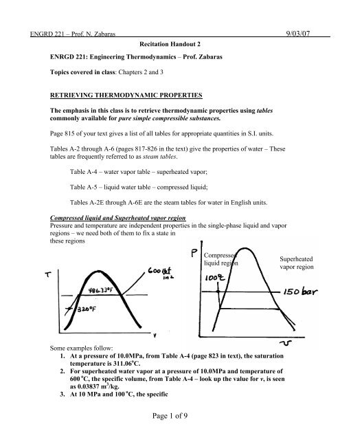
Compressed liquid and Superheated vapor region
Pressure and temperature are independent properties in the single-phase liquid and vapor
regions – we need both of them to fix a state in
these regions
Compressed
liquid region
Superheated
vapor region
Some examples follow:
1. At a pressure of 10.0MPa, from Table A-4 (page 823 in text), the saturation
temperature is 311.06 o C.
2. For superheated water vapor at a pressure of 10.0MPa and temperature of
600 o C, the specific volume, from Table A-4 – look up the value for v, is seen
as 0.03837 m 3 /kg.
3. At 10 MPa and 100 o C, the specific
Page 1 of 9

ENGRD 221 – Prof. N. Zabaras 9/03/07
volume of compressed water is – from
Table A-5 (page 825 in text) – 1.0385 x 10 -3 m 3 /kg. (Note that υ x 10 3 is given)
Saturated liquid and vapor region
The saturation tables A-2 and A-3 (pages
817-820 in text) list the properties of
saturated liquid and vapor states
The properties are denoted by subscripts f
and g to denote the fluid and gas,
respectively.
In the saturated liquid or vapor region, only
one property is necessary to fix the state –
This property is normally either the pressure
or the temperature - Table A-2 is called the
temperature table as the temperature is listed
in the first column while Table A-3 is called
the pressure table because pressures are
listed in convenient increments.
Compressed
liquid region
Saturated
liquid
vapor
region
x
Superheated
vapor region
What is quality? Quality is the ratio of the mass of vapor to the total mass of the closed
system. It is commonly denoted by x.
x = m gas /(m fluid + m gas )
If the quality is known, then the average specific volume of the saturated liquid – vapor
mixture is calculated as
v = (1-x) v f +x v g = v f + x(v g – v f )
For example:
Consider a system with a 2 – phase liquid-vapor mixture of water at 100 o C and a
quality of 0.9. From Table A-2, page 817 in text, looking up the column with
temperature=100 o C; we see that –
Specific
volume of
liquid (v f )
1.0435x10 -3
m 3 /kg
Specific
volume of
vapor (v g )
Internal
energy of
liquid (u f )
Internal
energy of
vapor (u g )
Enthalpy
of liquid
(h f )
Enthalpy
of vapor
(h f )
1.673 m 3 /kg 418.94 kJ/kg 2506.5 kJ/kg 419.04 kJ/kg 2676.1 kJ/kg
Therefore the specific volume of the mixture =
v = v f + x(v g – v f )
= 1.0435x10 -3 + 0.9*(1.673 - 1.0435x10 -3 )
= 1.506 m 3 /kg
Page 2 of 9

ENGRD 221 – Prof. N. Zabaras 9/03/07
Similarly, the average internal energy of the mixture is
u = u f + x(u g – u f )
= 418.94 + 0.9*(2506.5 – 418.94)
= 2297.75 kJ/kg
Enthalpy is defined - in chapter 3, page 89 in text – as
h = u + pv
and can be evaluated for the mixture with a given quality as
h = h f + x(h g – h f )
= 419.04 + 0.9*(2676.1 – 419.04)
= 2450.4 kJ/kg
Approximation for liquids using the saturated liquid data
There are methods that approximate the properties of the compressed liquids – they are
easier than using the compressed liquid tables (for example the compressed water table –
Table A-5).
Approximate the values of v, u at a given pressure, p and temperature, T by the
corresponding values of the saturated liquid at temperature T (these approximations
account for the fact of little pressure dependence of v and u);
v(p, T) = v f (T)
u(p, T) = u f (T)
The approximation of enthalpy is not the enthalpy at the saturated liquid but is a
correction defined as
h(p, T) = h f (T) + v f (T)*(p –p saturation )
See Section 3.10.1 for more details.
-----------------------------------------------------------------------------------------------------------
Page 3 of 9

ENGRD 221 – Prof. N. Zabaras 9/03/07
TYPICAL EXAMPLES OF POSSIBLE INPUTS AND OUTPUTS TO TABLES
1. Compressed liquid and Superheated vapor region
INPUT 1 INPUT 2 OUTPUT
Case 1 Pressure Specific volume Temperature
Case 2 Specific volume Temperature Pressure
Case 3 Pressure Temperature Specific volume
Most common case – Table A-4 for
superheated water vapor and
Table A-5 for compressed water
2. Saturated liquid and vapor region
INPUT OUTPUT 1 OUTPUT 2
Case 1
Specific volume of Pressure
Temperature
saturated liquid
and/or vapor. Not
the specific volume
of the mixture
Case 2 Pressure Temperature Specific volumes of
the saturated liquid
and vapor
Case 3 Temperature Pressure Specific volumes of
the saturated liquid
and vapor
Most common cases – Table A-3
for case 2 and Table A-2 for case 3
------------------------------------------------------------------------------------------------------------
Note: Many of the thermodynamic tables in your text list several other properties not
referred above. As we introduce these properties during the semester, you should be able
to think of many other imput/output use of these tables.
Page 4 of 9

ENGRD 221 – Prof. N. Zabaras 9/03/07
IDEAL GAS MODEL
pv = RT
Ideal gas equation of state
Alternative forms:
pV = mRT
(Substitute in v = V/m)
p v =
RT
v = v / M
R = R / M
M = Molecular Weight
pv = nRT
v = V / n
Enthalpy:
h = u + pv
pv = RT
u = u(T)
h = h(T) = u(T) + RT (Ideal Gas) (3.37)
Specific Internal Energy:
u depends only on temperature.
c v
T ) =
du
dT
( (Ideal Gas) (3.38)
uT ( ) uT ( ) c( T)
dT
2 1
T
T
2
− =∫
(Ideal Gas)
1
v
Specific Enthalpy:
h depends only on temperature.
c p
T ) =
dh
dT
( (Ideal Gas) (3.41)
hT ( ) hT ( ) c ( T)
dT
2 1
T
2
− =∫
T
1
p
(Ideal Gas)
Page 5 of 9

ENGRD 221 – Prof. N. Zabaras 9/03/07
By differentiating Eq 3.37 with respect to temperature, and plugging in Eq 3.38 & 3.41,
we can obtain
c
( T ) = c ( T ) R
(Ideal Gas) (3.44)
p v
+
Specific heat ratio k is a function of temperature only
k
c
p
( T )
= (Ideal Gas)
c ( T )
v
Combining with Eq 3.44 results in
c p (Ideal Gas)
kR
( T ) = k −1
R
( T ) = k −1
c v (Ideal Gas)
GENERALIZED COMPRESSIBILITY CHARTS
lim
p->
0
pv
T
= R
(1) , where R is a common limit for all ideal gases as p->0.
pv pv
We define compressibility factor as, Z = RT
= RT
, where Z is a dimensionless ratio.
Equation (1) is expressed in terms of the compressibility factor Z as lim Z = 1
When the pressure of a gas is relatively small compared to the critical pressure, P c ,
Z is approximately 1.
When coordinates of the compressibility plots of Z with p at different T are modified,
we obtain quantitatively similar plots for different gases.
When Z is plotted with reduced variables, T R and p R , defined as
p T
pR
= and TR
= ,
pc
Tc
generalized compressibility charts are obtained. Z = f(T R , p R ).
p->
0
Figures A1 – A3 (page 911-912) in text provide generalized charts where
where
v′
R
is called the pseudo specific volume.
v′ =
R
vpc
RT
c
Page 6 of 9

ENGRD 221 – Prof. N. Zabaras 9/03/07
Note: Absolute temperature (K) and absolute pressures should be used in
compressibility charts
Values of either T R or p R or
known.
v′
R
can be obtained from the plots if any two of them are
Some examples computing states from the thermodynamic tables:
Exercise:
1. Determine the specific volume of water at a state where p = 10bar and T = 215 C.
(ans. 0.2141 m
3 /kg)
2. Determine the temperature of water at a state of P = 0.5MPa and h= 2890 kJ / kg
. (ans. 216.4 C )
3
3. Using the tables for water, at p = 3 bar and v = 0.5 m / kg , find T in C and u in
kJ / kg . (ans. 133.6 C , 2196.7 kJ / kg )
4. Using the tables for water, at p = 4 Mpa andT =160 C, find v in m 3 / kg and u in
−3 3
kJ / kg . (ans. 1.1011 × 10 m / kg, 673.71 kJ / kg )
Page 7 of 9

ENGRD 221 – Prof. N. Zabaras 9/03/07
Problem 1:
• ∆U=U 2 -U 1
• W tot =W pw +W piston
Some hints related to the HW
Problem 2:
• UNITS!!! ->get everything in the same units right away!
• Adiabatic!
• Sign Convention
Problem 3:
• UNITS!
W
cycle
• η=
Q
in
Problem 4:
• Quasi-static---equilibrium…
• Yet again, unit conversion is a must
Problem 5:
• Use correct tables
• Interpolate
• Isothermal
Page 8 of 9

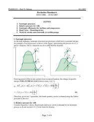
ENGRD 221 – Prof. N. Zabaras 9/03/07
Problem 6:
p
• pR
=
pc
vpc
• v′ R
=
RTc
T
• TR
=
Tc
8314Nm
• R=
32kgK
• Table A-1, fig A-2
Problem 7:
• C v =C p -R
• A-21E get C v (T)
• T2
uT ( ) uT ( ) c( T)
dT
− =∫
2 1
T1
Problem 8: To be discussed in class.
v
Page 9 of 9