A Short Tutorial on the Expectation-Maximization Algorithm - Snlp.de
A Short Tutorial on the Expectation-Maximization Algorithm - Snlp.de
A Short Tutorial on the Expectation-Maximization Algorithm - Snlp.de

Create successful ePaper yourself
Turn your PDF publications into a flip-book with our unique Google optimized e-Paper software.
A <str<strong>on</strong>g>Short</str<strong>on</strong>g> <str<strong>on</strong>g>Tutorial</str<strong>on</strong>g> <strong>on</strong> <strong>the</strong> Expectati<strong>on</strong>-Maximizati<strong>on</strong> <strong>Algorithm</strong><br />
Detlef Prescher<br />
Institute for Logic, Language and Computati<strong>on</strong><br />
University of Amsterdam<br />
prescher@science.uva.nl<br />
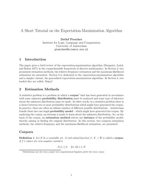
1 Introducti<strong>on</strong><br />
The paper gives a brief review of <strong>the</strong> expectati<strong>on</strong>-maximizati<strong>on</strong> algorithm (Dempster, Laird,<br />
and Rubin 1977) in <strong>the</strong> comprehensible framework of discrete ma<strong>the</strong>matics. In Secti<strong>on</strong> 2, two<br />
prominent estimati<strong>on</strong> methods, <strong>the</strong> relative-frequency estimati<strong>on</strong> and <strong>the</strong> maximum-likelihood<br />
estimati<strong>on</strong> are presented. Secti<strong>on</strong> 3 is <strong>de</strong>dicated to <strong>the</strong> expectati<strong>on</strong>-maximizati<strong>on</strong> algorithm<br />
and a simpler variant, <strong>the</strong> generalized expectati<strong>on</strong>-maximizati<strong>on</strong> algorithm. In Secti<strong>on</strong> 4, two<br />
loa<strong>de</strong>d dice are rolled. Enjoy!<br />
2 Estimati<strong>on</strong> Methods<br />
A statistics problem is a problem in which a corpus 1 that has been generated in accordance<br />
with some unknown probability distributi<strong>on</strong> must be analyzed and some type of inference<br />
about <strong>the</strong> unknown distributi<strong>on</strong> must be ma<strong>de</strong>. In o<strong>the</strong>r words, in a statistics problem <strong>the</strong>re is<br />
a choice between two or more probability distributi<strong>on</strong>s which might have generated <strong>the</strong> corpus.<br />
In practice, <strong>the</strong>re are often an infinite number of different possible distributi<strong>on</strong>s – statisticians<br />
bundle <strong>the</strong>se into <strong>on</strong>e single probability mo<strong>de</strong>l – which might have generated <strong>the</strong> corpus. By<br />
analyzing <strong>the</strong> corpus, an attempt is ma<strong>de</strong> to learn about <strong>the</strong> unknown distributi<strong>on</strong>. So, <strong>on</strong> <strong>the</strong><br />
basis of <strong>the</strong> corpus, an estimati<strong>on</strong> method selects <strong>on</strong>e instance of <strong>the</strong> probability mo<strong>de</strong>l,<br />
<strong>the</strong>reby aiming at finding <strong>the</strong> original distributi<strong>on</strong>. In this secti<strong>on</strong>, two comm<strong>on</strong> estimati<strong>on</strong><br />
methods, <strong>the</strong> relative-frequency and <strong>the</strong> maximum-likelihood estimati<strong>on</strong>, are presented.<br />
Corpora<br />
Definiti<strong>on</strong> 1 Let X be a countable set. A real-valued functi<strong>on</strong> f : X → R is called a corpus,<br />
if f’s values are n<strong>on</strong>-negative numbers<br />
f(x) ≥ 0<br />
for all x ∈ X<br />
1 Statisticians use <strong>the</strong> term sample but computati<strong>on</strong>al linguists prefer <strong>the</strong> term corpus<br />
1
Each x ∈ X is called a type, and each value of f is called a type frequency. The corpus<br />
size 2 is <strong>de</strong>fined as<br />
|f| = ∑ f(x)<br />
x∈X<br />
Finally, a corpus is called n<strong>on</strong>-empty and finite if<br />
0 < |f| < ∞<br />
In this <strong>de</strong>finiti<strong>on</strong>, type frequencies are <strong>de</strong>fined as n<strong>on</strong>-negative real numbers. The reas<strong>on</strong> for<br />
not taking natural numbers is that some statistical estimati<strong>on</strong> methods <strong>de</strong>fine type frequencies<br />
as weighted occurrence frequencies (which are not natural but n<strong>on</strong>-negative real numbers).<br />
Later <strong>on</strong>, in <strong>the</strong> c<strong>on</strong>text of <strong>the</strong> EM algorithm, this point will become clear. Note also that<br />
a finite corpus might c<strong>on</strong>sist of an infinite number of types with positive frequencies. The<br />
following <strong>de</strong>finiti<strong>on</strong> shows that Definiti<strong>on</strong> 1 covers <strong>the</strong> standard noti<strong>on</strong> of <strong>the</strong> term corpus<br />
(used in Computati<strong>on</strong>al Linguistics) and of <strong>the</strong> term sample (used in Statistics).<br />
Definiti<strong>on</strong> 2 Let x 1 , . . . , x n be a finite sequence of type instances from X . Each x i of this<br />
sequence is called a token. The occurrence frequency of a type x in <strong>the</strong> sequence is <strong>de</strong>fined<br />
as <strong>the</strong> following count<br />
f(x) = | { i | x i = x} |<br />
Obviously, f is a corpus in <strong>the</strong> sense of Definiti<strong>on</strong> 1, and it has <strong>the</strong> following properties: The<br />
type x does not occur in <strong>the</strong> sequence if f(x) = 0; In any o<strong>the</strong>r case <strong>the</strong>re are f(x) tokens<br />
in <strong>the</strong> sequence which are i<strong>de</strong>ntical to x. Moreover, <strong>the</strong> corpus size |f| is i<strong>de</strong>ntical to n, <strong>the</strong><br />
number of tokens in <strong>the</strong> sequence.<br />
Relative-Frequency Estimati<strong>on</strong><br />
Let us first present <strong>the</strong> noti<strong>on</strong> of probability that we use throughout this paper.<br />
Definiti<strong>on</strong> 3 Let X be a countable set of types. A real-valued functi<strong>on</strong> p: X → R is called a<br />
probability distributi<strong>on</strong> <strong>on</strong> X , if p has two properties: First, p’s values are n<strong>on</strong>-negative<br />
numbers<br />
p(x) ≥ 0 for all x ∈ X<br />
and sec<strong>on</strong>d, p’s values sum to 1<br />
∑<br />
p(x) = 1<br />
x∈X<br />
Rea<strong>de</strong>rs familiar to probability <strong>the</strong>ory will certainly note that we use <strong>the</strong> term probability<br />
distributi<strong>on</strong> in a sloppy way (Duda et al. (2001), page 611, introduce <strong>the</strong> term probability<br />
mass functi<strong>on</strong> instead). Standardly, probability distributi<strong>on</strong>s allocate a probability value p(A)<br />
to subsets A ⊆ X , so-called events of an event space X , such that three specific axioms are<br />
satisfied (see e.g. DeGroot (1989)):<br />
Axiom 1 p(A) ≥ 0 for any event A.<br />
2 Note that <strong>the</strong> corpus size |f| is well-<strong>de</strong>fined: The or<strong>de</strong>r of summati<strong>on</strong> is not relevant for <strong>the</strong> value of <strong>the</strong><br />
(possible infinite) series ∑ f(x), since <strong>the</strong> types are countable and <strong>the</strong> type frequencies are n<strong>on</strong>-negative<br />
x∈X<br />
numbers<br />
2
corpus of<br />
data<br />
probability<br />
mo<strong>de</strong>l<br />
an instance<br />
of <strong>the</strong> probability mo<strong>de</strong>l<br />
maximizing<br />
<strong>the</strong> corpus probability<br />
(input)<br />
Maximum−Likelihood Estimati<strong>on</strong><br />
(output)<br />
corpus of<br />
data<br />
<strong>the</strong> probability distributi<strong>on</strong><br />
comprising<br />
<strong>the</strong> relative frequencies<br />
of <strong>the</strong> corpus types<br />
(input)<br />
Relative−Frequency Estimati<strong>on</strong><br />
(output)<br />
Figure 1: Maximum-likelihood estimati<strong>on</strong> and relative-frequency estimati<strong>on</strong><br />
Axiom 2 p(X ) = 1.<br />
Axiom 3 p( ⋃ ∞<br />
i=1 A i ) = ∑ ∞<br />
i=1 p(A i ) for any infinite sequence of disjoint events A 1 , A 2 , A 3 , ...<br />
Now, however, note that <strong>the</strong> probability distributi<strong>on</strong>s introduced in Definiti<strong>on</strong> 3 induce ra<strong>the</strong>r<br />
naturally <strong>the</strong> following probabilities for events A ⊆ X<br />
p(A) := ∑ x∈A<br />
p(x)<br />
Using <strong>the</strong> properties of p(x), we can easily show that <strong>the</strong> probabilities p(A) satisfy <strong>the</strong> three<br />
axioms of probability <strong>the</strong>ory. So, Definiti<strong>on</strong> 3 is justified and thus, for <strong>the</strong> rest of <strong>the</strong> paper,<br />
we are allowed to put axiomatic probability <strong>the</strong>ory out of our minds.<br />
Definiti<strong>on</strong> 4 Let f be a n<strong>on</strong>-empty and finite corpus. The probability distributi<strong>on</strong><br />
˜p: X → [0, 1] where ˜p(x) = f(x)<br />
|f|<br />
is called <strong>the</strong> relative-frequency estimate <strong>on</strong> f.<br />
The relative-frequency estimati<strong>on</strong> is <strong>the</strong> most comprehensible estimati<strong>on</strong> method and has<br />
some nice properties which will be discussed in <strong>the</strong> c<strong>on</strong>text of <strong>the</strong> more general maximumlikelihood<br />
estimati<strong>on</strong>. For now, however, note that ˜p is well <strong>de</strong>fined, since both |f| > 0<br />
and |f| < ∞.<br />
∑x∈X |f|−1 · f(x) = |f| −1 · ∑<br />
x∈X f(x) = |f|−1 · |f| = 1.<br />
Moreover, it is easy to check that ˜p’s values sum to <strong>on</strong>e:<br />
Maximum-Likelihood Estimati<strong>on</strong><br />
∑<br />
x∈X ˜p(x) =<br />
Maximum-likelihood estimati<strong>on</strong> was introduced by R. A. Fisher in 1912, and will typically<br />
yield an excellent estimate if <strong>the</strong> given corpus is large. Most notably, maximum-likelihood<br />
estimators fulfill <strong>the</strong> so-called invariance principle and, un<strong>de</strong>r certain c<strong>on</strong>diti<strong>on</strong>s which<br />
3
are typically satisfied in practical problems, <strong>the</strong>y are even c<strong>on</strong>sistent estimators (DeGroot<br />
1989). For <strong>the</strong>se reas<strong>on</strong>s, maximum-likelihood estimati<strong>on</strong> is probably <strong>the</strong> most wi<strong>de</strong>ly used<br />
estimati<strong>on</strong> method.<br />
Now, unlike relative-frequency estimati<strong>on</strong>, maximum-likelihood estimati<strong>on</strong> is a fully-fledged<br />
estimati<strong>on</strong> method that aims at selecting an instance of a given probability mo<strong>de</strong>l which<br />
might have originally generated <strong>the</strong> given corpus. By c<strong>on</strong>trast, <strong>the</strong> relative-frequency estimate<br />
is <strong>de</strong>fined <strong>on</strong> <strong>the</strong> basis of a corpus <strong>on</strong>ly (see Definiti<strong>on</strong> 4). Figure 1 reveals <strong>the</strong> c<strong>on</strong>ceptual<br />
difference of both estimati<strong>on</strong> methods. In what follows, we will pay some attenti<strong>on</strong> to <strong>de</strong>scribe<br />
<strong>the</strong> single setting, in which we are excepti<strong>on</strong>ally allowed to mix up both methods (see<br />
Theorem 1). Let us start, however, by presenting <strong>the</strong> noti<strong>on</strong> of a probability mo<strong>de</strong>l.<br />
Definiti<strong>on</strong> 5 A n<strong>on</strong>-empty set M of probability distributi<strong>on</strong>s <strong>on</strong> a set X of types is called a<br />
probability mo<strong>de</strong>l <strong>on</strong> X . The elements of M are called instances of <strong>the</strong> mo<strong>de</strong>l M. The<br />
unrestricted probability mo<strong>de</strong>l is <strong>the</strong> set M(X ) of all probability distributi<strong>on</strong>s <strong>on</strong> <strong>the</strong> set<br />
of types<br />
{<br />
}<br />
∑<br />
M(X ) = p: X → [0, 1]<br />
p(x) = 1<br />
∣<br />
x∈X<br />
A probability mo<strong>de</strong>l M is called restricted in all o<strong>the</strong>r cases<br />
M ⊆ M(X ) and M ≠ M(X )<br />
In practice, most probability mo<strong>de</strong>ls are restricted since <strong>the</strong>ir instances are often <strong>de</strong>fined <strong>on</strong> a<br />
set X comprising multi-dimensi<strong>on</strong>al types such that certain parts of <strong>the</strong> types are statistically<br />
in<strong>de</strong>pen<strong>de</strong>nt (see examples 4 and 5). Here is ano<strong>the</strong>r si<strong>de</strong> note: We already checked that<br />
<strong>the</strong> relative-frequency estimate is a probability distributi<strong>on</strong>, meaning in terms of Definiti<strong>on</strong> 5<br />
that <strong>the</strong> relative-frequency estimate is an instance of <strong>the</strong> unrestricted probability mo<strong>de</strong>l. So,<br />
from an extreme point of view, <strong>the</strong> relative-frequency estimati<strong>on</strong> might be also regar<strong>de</strong>d as<br />
a fully-fledged estimati<strong>on</strong> method exploiting a corpus and a probability mo<strong>de</strong>l (namely, <strong>the</strong><br />
unrestricted mo<strong>de</strong>l).<br />
In <strong>the</strong> following, we <strong>de</strong>fine maximum-likelihood estimati<strong>on</strong> as a method that aims at<br />
finding an instance of a given mo<strong>de</strong>l which maximizes <strong>the</strong> probability of a given corpus.<br />
Later <strong>on</strong>, we will see that maximum-likelihood estimates have an additi<strong>on</strong>al property: They<br />
are <strong>the</strong> instances of <strong>the</strong> given probability mo<strong>de</strong>l that have a “minimal distance” to <strong>the</strong> relative<br />
frequencies of <strong>the</strong> types in <strong>the</strong> corpus (see Theorem 2). So, in<strong>de</strong>ed, maximum-likelihood<br />
estimates can be intuitively thought of in <strong>the</strong> inten<strong>de</strong>d way: They are <strong>the</strong> instances of <strong>the</strong><br />
probability mo<strong>de</strong>l that might have originally generated <strong>the</strong> corpus.<br />
Definiti<strong>on</strong> 6 Let f be a n<strong>on</strong>-empty and finite corpus <strong>on</strong> a countable set X of types. Let M<br />
be a probability mo<strong>de</strong>l <strong>on</strong> X . The probability of <strong>the</strong> corpus allocated by an instance p of<br />
<strong>the</strong> mo<strong>de</strong>l M is <strong>de</strong>fined as<br />
L(f; p) = ∏<br />
p(x) f(x)<br />
x∈X<br />
An instance ˆp of <strong>the</strong> mo<strong>de</strong>l M is called a maximum-likelihood estimate of M <strong>on</strong> f, if<br />
and <strong>on</strong>ly if <strong>the</strong> corpus f is allocated a maximum probability by ˆp<br />
L(f; ˆp) = max L(f; p)<br />
p∈M<br />
(Based <strong>on</strong> c<strong>on</strong>tinuity arguments, we use <strong>the</strong> c<strong>on</strong>venti<strong>on</strong> that p 0 = 1 and 0 0 = 1.)<br />
4
~<br />
p = ^p<br />
M<br />
M(X)<br />
p<br />
~<br />
M<br />
M(X)<br />
p^<br />
? ?<br />
Figure 2: Maximum-likelihood estimati<strong>on</strong> and relative-frequency estimati<strong>on</strong> yield for some “excepti<strong>on</strong>al”<br />
probability mo<strong>de</strong>ls <strong>the</strong> same estimate. These mo<strong>de</strong>ls are lightly restricted or even unrestricted<br />
mo<strong>de</strong>ls that c<strong>on</strong>tain an instance comprising <strong>the</strong> relative frequencies of all corpus types (left-hand si<strong>de</strong>).<br />
In practice, however, most probability mo<strong>de</strong>ls will not behave like that. So, maximum-likelihood estimati<strong>on</strong><br />
and relative-frequency estimati<strong>on</strong> yield in most cases different estimates. As a fur<strong>the</strong>r and<br />
more serious c<strong>on</strong>sequence, <strong>the</strong> maximum-likelihood estimates have <strong>the</strong>n to be searched for by genuine<br />
optimizati<strong>on</strong> procedures (right-hand si<strong>de</strong>).<br />
By looking at this <strong>de</strong>finiti<strong>on</strong>, we recognize that maximum-likelihood estimates are <strong>the</strong> soluti<strong>on</strong>s<br />
of a quite complex optimizati<strong>on</strong> problem. So, some nasty questi<strong>on</strong>s about maximumlikelihood<br />
estimati<strong>on</strong> arise:<br />
Existence Is <strong>the</strong>re for any probability mo<strong>de</strong>l and any corpus a maximum-likelihood<br />
estimate of <strong>the</strong> mo<strong>de</strong>l <strong>on</strong> <strong>the</strong> corpus?<br />
Uniqueness Is <strong>the</strong>re for any probability mo<strong>de</strong>l and any corpus a unique maximumlikelihood<br />
estimate of <strong>the</strong> mo<strong>de</strong>l <strong>on</strong> <strong>the</strong> corpus?<br />
Computability For which probability mo<strong>de</strong>ls and corpora can maximum-likelihood<br />
estimates be efficiently computed?<br />
For some probability mo<strong>de</strong>ls M, <strong>the</strong> following <strong>the</strong>orem gives a positive answer.<br />
Theorem 1 Let f be a n<strong>on</strong>-empty and finite corpus <strong>on</strong> a countable set X of types. Then:<br />
(i) The relative-frequency estimate ˜p is a unique maximum-likelihood estimate of <strong>the</strong> unrestricted<br />
probability mo<strong>de</strong>l M(X ) <strong>on</strong> f.<br />
(ii) The relative-frequency estimate ˜p is a maximum-likelihood estimate of a (restricted or<br />
unrestricted) probability mo<strong>de</strong>l M <strong>on</strong> f, if and <strong>on</strong>ly if ˜p is an instance of <strong>the</strong> mo<strong>de</strong>l M.<br />
In this case, ˜p is a unique maximum-likelihood estimate of M <strong>on</strong> f.<br />
Proof Ad (i): Combine <strong>the</strong>orems 2 and 3. Ad (ii): “⇒” is trivial. “⇐” by (i) q.e.d.<br />
On a first glance, propositi<strong>on</strong> (ii) seems to be more general than propositi<strong>on</strong> (i), since propositi<strong>on</strong><br />
(i) is about <strong>on</strong>e single probability mo<strong>de</strong>l, <strong>the</strong> unrestricted mo<strong>de</strong>l, whereas propositi<strong>on</strong><br />
(ii) gives some insight about <strong>the</strong> relati<strong>on</strong> of <strong>the</strong> relative-frequency estimate to a maximumlikelihood<br />
estimate of arbitrary restricted probability mo<strong>de</strong>ls (see also Figure 2). Both propositi<strong>on</strong>s,<br />
however, are equivalent. As we will show later <strong>on</strong>, propositi<strong>on</strong> (i) is equivalent to<br />
<strong>the</strong> famous informati<strong>on</strong> inequality of informati<strong>on</strong> <strong>the</strong>ory, for which various proofs have been<br />
given in <strong>the</strong> literature.<br />
5
Example 1 On <strong>the</strong> basis of <strong>the</strong> following corpus<br />
f(a) = 2, f(b) = 3, f(c) = 5<br />
we shall calculate <strong>the</strong> maximum-likelihood estimate of <strong>the</strong> unrestricted probability mo<strong>de</strong>l<br />
M({a, b, c}), as well as <strong>the</strong> maximum-likelihood estimate of <strong>the</strong> restricted probability mo<strong>de</strong>l<br />
M =<br />
{<br />
}<br />
p ∈ M({a, b, c}) ∣ p(a) = 0.5<br />
The soluti<strong>on</strong> is instructive, but is left to <strong>the</strong> rea<strong>de</strong>r.<br />
The Informati<strong>on</strong> Inequality of Informati<strong>on</strong> Theory<br />
Definiti<strong>on</strong> 7 The relative entropy D(p || q) of <strong>the</strong> probability distributi<strong>on</strong> p with respect<br />
to <strong>the</strong> probability distributi<strong>on</strong> q is <strong>de</strong>fined by<br />
D(p || q) = ∑ x∈X<br />
p(x) log p(x)<br />
q(x)<br />
(Based <strong>on</strong> c<strong>on</strong>tinuity arguments, we use <strong>the</strong> c<strong>on</strong>venti<strong>on</strong> that 0 log 0 q = 0 and p log p 0 = ∞ and<br />
0 log 0 0<br />
= 0. The logarithm is calculated with respect to <strong>the</strong> base 2.)<br />
C<strong>on</strong>necting maximum-likelihood estimati<strong>on</strong> with <strong>the</strong> c<strong>on</strong>cept of relative entropy, <strong>the</strong> following<br />
<strong>the</strong>orem gives <strong>the</strong> important insight that <strong>the</strong> relative-entropy of <strong>the</strong> relative-frequency<br />
estimate is minimal with respect to a maximum-likelihood estimate.<br />
Theorem 2 Let ˜p be <strong>the</strong> relative-frequency estimate <strong>on</strong> a n<strong>on</strong>-empty and finite corpus f, and<br />
let M be a probability mo<strong>de</strong>l <strong>on</strong> <strong>the</strong> set X of types. Then: An instance ˆp of <strong>the</strong> mo<strong>de</strong>l M is<br />
a maximum-likelihood estimate of M <strong>on</strong> f, if and <strong>on</strong>ly if <strong>the</strong> relative-entropy of ˜p is minimal<br />
with respect to ˆp<br />
D(˜p || ˆp) = min D(˜p || p)<br />
p∈M<br />
Proof First, <strong>the</strong> relative entropy D(˜p || p) is simply <strong>the</strong> difference of two fur<strong>the</strong>r entropy<br />
values, <strong>the</strong> so-called cross-entropy H(˜p; p) = − ∑ x∈X ˜p(x) log p(x) and <strong>the</strong> entropy H(˜p) =<br />
− ∑ x∈X ˜p(x) log ˜p(x) of <strong>the</strong> relative-frequency estimate<br />
D(˜p || p) = H(˜p; p) − H(˜p)<br />
(Based <strong>on</strong> c<strong>on</strong>tinuity arguments and in full agreement with <strong>the</strong> c<strong>on</strong>venti<strong>on</strong> used in Definiti<strong>on</strong> 7,<br />
we use here that ˜p log 0 = −∞ and 0 log 0 = 0.) It follows that minimizing <strong>the</strong> relative<br />
entropy is equivalent to minimizing <strong>the</strong> cross-entropy (as a functi<strong>on</strong> of <strong>the</strong> instances p of<br />
<strong>the</strong> given probability mo<strong>de</strong>l M). The cross-entropy, however, is proporti<strong>on</strong>al to <strong>the</strong> negative<br />
log-probability of <strong>the</strong> corpus f<br />
H(˜p; p) = − 1 log L(f; p)<br />
|f|<br />
6
So, finally, minimizing <strong>the</strong> relative entropy D(˜p || p) is equivalent to maximizing <strong>the</strong> corpus<br />
probability L(f; p). 3<br />
Toge<strong>the</strong>r with Theorem 2, <strong>the</strong> following <strong>the</strong>orem, <strong>the</strong> so-called informati<strong>on</strong> inequality of<br />
informati<strong>on</strong> <strong>the</strong>ory, proves Theorem 1. The informati<strong>on</strong> inequality states simply that <strong>the</strong><br />
relative entropy is a n<strong>on</strong>-negative number – which is zero, if and <strong>on</strong>ly if <strong>the</strong> two probability<br />
distributi<strong>on</strong>s are equal.<br />
Theorem 3 (Informati<strong>on</strong> Inequality) Let p and q be two probability distributi<strong>on</strong>s. Then<br />
D(p || q) ≥ 0<br />
with equality if and <strong>on</strong>ly if p(x) = q(x) for all x ∈ X .<br />
Proof See, e.g., Cover and Thomas (1991), page 26.<br />
*Maximum-Entropy Estimati<strong>on</strong><br />
Rea<strong>de</strong>rs <strong>on</strong>ly interested in <strong>the</strong> expectati<strong>on</strong>-maximizati<strong>on</strong> algorithm are encouraged to omit<br />
this secti<strong>on</strong>. For completeness, however, note that <strong>the</strong> relative entropy is asymmetric. That<br />
means, in general<br />
D(p||q) ≠ D(q||p)<br />
It is easy to check that <strong>the</strong> triangle inequality is not valid too. So, <strong>the</strong> relative entropy D(.||.)<br />
is not a “true” distance functi<strong>on</strong>. On <strong>the</strong> o<strong>the</strong>r hand, D(.||.) has some of <strong>the</strong> properties of a<br />
distance functi<strong>on</strong>. In particular, it is always n<strong>on</strong>-negative and it is zero if and <strong>on</strong>ly if p = q<br />
(see Theorem 3). So far, however, we aimed at minimizing <strong>the</strong> relative entropy with respect<br />
to its sec<strong>on</strong>d argument, filling <strong>the</strong> first argument slot of D(.||.) with <strong>the</strong> relative-frequency<br />
estimate ˜p. Obviously, <strong>the</strong>se observati<strong>on</strong>s raise <strong>the</strong> questi<strong>on</strong>, whe<strong>the</strong>r it is also possible to<br />
<strong>de</strong>rive o<strong>the</strong>r “good” estimates by minimizing <strong>the</strong> relative entropy with respect to its first<br />
argument. So, in terms of Theorem 2, it might be interesting to ask for mo<strong>de</strong>l instances<br />
p ∗ ∈ M with<br />
D(p ∗ ||˜p) = min<br />
p∈M D(p||˜p)<br />
For at least two reas<strong>on</strong>s, however, this initial approach of relative-entropy estimati<strong>on</strong> is too<br />
simplistic. First, it is tailored to probability mo<strong>de</strong>ls that lack any generalizati<strong>on</strong> power.<br />
Sec<strong>on</strong>d, it does not provi<strong>de</strong> <strong>de</strong>eper insight when estimating c<strong>on</strong>strained probability mo<strong>de</strong>ls.<br />
Here are <strong>the</strong> <strong>de</strong>tails:<br />
3 For completeness, note that <strong>the</strong> perplexity of a corpus f allocated by a mo<strong>de</strong>l instance p is <strong>de</strong>fined as<br />
√<br />
(<br />
|f|<br />
perp(f; p) = 2 H(˜p;p) . This yields perp(f; p) = |f| 1<br />
and L(f; p) = 1<br />
L(f;p) perp(f;p))<br />
as well as <strong>the</strong> comm<strong>on</strong><br />
interpretati<strong>on</strong> that <strong>the</strong> perplexity value measures <strong>the</strong> complexity of <strong>the</strong> given corpus from <strong>the</strong><br />
mo<strong>de</strong>l instance’s view: <strong>the</strong> perplexity is equal to <strong>the</strong> size of an imaginary word list from which <strong>the</strong> corpus<br />
can be generated by <strong>the</strong> mo<strong>de</strong>l instance – assuming that all words <strong>on</strong> this list are equally probable. Moreover,<br />
<strong>the</strong> equati<strong>on</strong>s state that minimizing <strong>the</strong> corpus perplexity perp(f; p) is equivalent to maximizing <strong>the</strong> corpus<br />
probability L(f; p).<br />
7
• A closer look at Definiti<strong>on</strong> 7 reveals that <strong>the</strong> relative entropy D(p||˜p) is finite for those<br />
mo<strong>de</strong>l instances p ∈ M <strong>on</strong>ly that fulfill<br />
˜p(x) = 0 ⇒ p(x) = 0<br />
So, <strong>the</strong> initial approach would lead to mo<strong>de</strong>l instances that are completely unable to<br />
generalize, since <strong>the</strong>y are not allowed to allocate positive probabilities to at least some<br />
of <strong>the</strong> types not seen in <strong>the</strong> training corpus.<br />
• Theorem 2 guarantees that <strong>the</strong> relative-frequency estimate ˜p is a soluti<strong>on</strong> to <strong>the</strong> initial<br />
approach of relative-entropy estimati<strong>on</strong>, whenever ˜p ∈ M. Now, Definiti<strong>on</strong> 8 introduces<br />
<strong>the</strong> c<strong>on</strong>strained probability mo<strong>de</strong>ls M c<strong>on</strong>str , and in<strong>de</strong>ed, it is easy to check that ˜p is<br />
always an instance of <strong>the</strong>se mo<strong>de</strong>ls. In o<strong>the</strong>r words, estimating c<strong>on</strong>strained probability<br />
mo<strong>de</strong>ls by <strong>the</strong> approach above does not result in interesting mo<strong>de</strong>l instances.<br />
Clearly, all <strong>the</strong> menti<strong>on</strong>ed drawbacks are due to <strong>the</strong> fact that <strong>the</strong> relative-entropy minimizati<strong>on</strong><br />
is performed with respect to <strong>the</strong> relative-frequency estimate. As a resource, we switch simply<br />
to a more c<strong>on</strong>venient reference distributi<strong>on</strong>, <strong>the</strong>reby generalizing formally <strong>the</strong> initial problem<br />
setting. So, as <strong>the</strong> final request, we ask for mo<strong>de</strong>l instances p ∗ ∈ M with<br />
D(p ∗ ||p 0 ) = min<br />
p∈M D(p||p 0)<br />
In this setting, <strong>the</strong> reference distributi<strong>on</strong> p 0 ∈ M(X ) is a given instance of <strong>the</strong> unrestricted<br />
probability mo<strong>de</strong>l, and from what we have seen so far, p 0 should allocate all types of interest<br />
a positive probability, and moreover, p 0 should not be itself an instance of <strong>the</strong> probability<br />
mo<strong>de</strong>l M. In<strong>de</strong>ed, this request will lead us to <strong>the</strong> interesting maximum-entropy estimates.<br />
Note first, that<br />
D(p||p 0 ) = H(p; p 0 ) − H(p)<br />
So, minimizing D(p||p 0 ) as a functi<strong>on</strong> of <strong>the</strong> mo<strong>de</strong>l instances p is equivalent to minimizing<br />
<strong>the</strong> cross entropy H(p; p 0 ) and simultaneously maximizing <strong>the</strong> mo<strong>de</strong>l entropy H(p). Now,<br />
simultaneous optimizati<strong>on</strong> is a hard task in general, and this gives reas<strong>on</strong> to focus firstly<br />
<strong>on</strong> maximizing <strong>the</strong> entropy H(p) in isolati<strong>on</strong>. The following <strong>de</strong>finiti<strong>on</strong> presents maximumentropy<br />
estimati<strong>on</strong> in terms of <strong>the</strong> well-known maximum-entropy principle (Jaynes 1957).<br />
Sloppily formulated, <strong>the</strong> maximum-entropy principle recommends to maximize <strong>the</strong> entropy<br />
H(p) as a functi<strong>on</strong> of <strong>the</strong> instances p of certain “c<strong>on</strong>strained” probability mo<strong>de</strong>ls.<br />
Definiti<strong>on</strong> 8 Let f 1 , . . . , f d be a finite number of real-valued functi<strong>on</strong>s <strong>on</strong> a set X of types,<br />
<strong>the</strong> so-called feature functi<strong>on</strong>s 4 . Let ˜p be <strong>the</strong> relative-frequency estimate <strong>on</strong> a n<strong>on</strong>-empty<br />
4 Each of <strong>the</strong>se feature functi<strong>on</strong>s can be thought of as being c<strong>on</strong>structed by inspecting <strong>the</strong> set of types,<br />
<strong>the</strong>reby measuring a specific property of <strong>the</strong> types x ∈ X . For example, if working in a formal-grammar<br />
framework, <strong>the</strong>n it might be worthy to look (at least) at some feature functi<strong>on</strong>s f r directly associated to <strong>the</strong><br />
rules r of <strong>the</strong> given formal grammar. The “measure” f r(x) of a specific rule r for <strong>the</strong> analyzes x ∈ X of <strong>the</strong><br />
grammar might be calculated, for example, in terms of <strong>the</strong> occurrence frequency of r in <strong>the</strong> sequence of those<br />
rules which are necessary to produce x. For instance, Chi (1999) studied this approach for <strong>the</strong> c<strong>on</strong>text-free<br />
grammar formalism. Note, however, that <strong>the</strong>re is in general no recipe for c<strong>on</strong>structing “good” feature functi<strong>on</strong>s:<br />
Often, it is really an intellectual challenge to find those feature functi<strong>on</strong>s that <strong>de</strong>scribe <strong>the</strong> given data as best<br />
as possible (or at least in a satisfying manner).<br />
8
and finite corpus f <strong>on</strong> X . Then, <strong>the</strong> probability mo<strong>de</strong>l c<strong>on</strong>strained by <strong>the</strong> expected<br />
values of f 1 . . . f d <strong>on</strong> f is <strong>de</strong>fined as<br />
{<br />
}<br />
M c<strong>on</strong>str = p ∈ M(X )<br />
E<br />
∣ p f i = E˜p f i for i = 1, . . . , d<br />
Here, each E p f i is <strong>the</strong> mo<strong>de</strong>l instance’s expectati<strong>on</strong> of f i<br />
E p f i = ∑ p(x)f i (x)<br />
x∈X<br />
c<strong>on</strong>strained to match E˜p f i , <strong>the</strong> observed expectati<strong>on</strong> of f i<br />
E˜p f i = ∑ x∈X<br />
˜p(x)f i (x)<br />
Fur<strong>the</strong>rmore, a mo<strong>de</strong>l instance p ∗ ∈ M c<strong>on</strong>str is called a maximum-entropy estimate of<br />
M c<strong>on</strong>str if and <strong>on</strong>ly if<br />
H(p ∗ ) = max H(p)<br />
p∈M c<strong>on</strong>str<br />
It is well-known that <strong>the</strong> maximum-entropy estimates have some nice properties. For example,<br />
as Definiti<strong>on</strong> 9 and Theorem 4 show, <strong>the</strong>y can be i<strong>de</strong>ntified to be <strong>the</strong> unique maximumlikelihood<br />
estimates of <strong>the</strong> so-called exp<strong>on</strong>ential mo<strong>de</strong>ls (which are also known as log-linear<br />
mo<strong>de</strong>ls).<br />
Definiti<strong>on</strong> 9 Let f 1 , . . . , f d be a finite number of feature functi<strong>on</strong>s <strong>on</strong> a set X of types. The<br />
exp<strong>on</strong>ential mo<strong>de</strong>l of f 1 , . . . , f d is <strong>de</strong>fined by<br />
{<br />
M exp = p ∈ M(X )<br />
p(x) = 1 }<br />
e λ 1f 1 (x)+...+λ d f d (x) with λ<br />
∣<br />
1 , . . . , λ d , Z λ ∈ R<br />
Z λ<br />
Here, <strong>the</strong> normalizing c<strong>on</strong>stant Z λ (with λ as a short form for <strong>the</strong> sequence λ 1 , . . . , λ d )<br />
guarantees that p ∈ M(X ), and it is given by<br />
Z λ = ∑ x∈X<br />
e λ 1f 1 (x)+...+λ d f d (x)<br />
Theorem 4 Let f be a n<strong>on</strong>-empty and finite corpus, and f 1 , . . . , f d be a finite number of<br />
feature functi<strong>on</strong>s <strong>on</strong> a set X of types. Then<br />
(i) The maximum-entropy estimates of M c<strong>on</strong>str are instances of M exp , and <strong>the</strong> maximumlikelihood<br />
estimates of M exp <strong>on</strong> f are instances of M c<strong>on</strong>str .<br />
(ii) If p ∗ ∈ M c<strong>on</strong>str ∩ M exp , <strong>the</strong>n p ∗ is both a unique maximum-entropy estimate of M c<strong>on</strong>str<br />
and a unique maximum-likelihood estimate of M exp <strong>on</strong> f.<br />
Part (i) of <strong>the</strong> <strong>the</strong>orem simply suggests <strong>the</strong> form of <strong>the</strong> maximum-entropy or maximumlikelihood<br />
estimates we are looking for. By combining both findings of (i), however, <strong>the</strong><br />
search space is drastically reduced for both estimati<strong>on</strong> methods: We simply have to look at<br />
<strong>the</strong> intersecti<strong>on</strong> of <strong>the</strong> involved probability mo<strong>de</strong>ls. In turn, exactly this fact makes <strong>the</strong> sec<strong>on</strong>d<br />
part of <strong>the</strong> <strong>the</strong>orem so valuable. If <strong>the</strong>re is a maximum-entropy or a maximum-likelihood<br />
9
maximum-likelihood<br />
estimati<strong>on</strong><br />
of<br />
⎧<br />
⎪⎨<br />
⎪⎩<br />
arbitrary probability mo<strong>de</strong>ls<br />
exp<strong>on</strong>ential mo<strong>de</strong>ls<br />
exp<strong>on</strong>ential mo<strong>de</strong>ls<br />
with reference distributi<strong>on</strong>s<br />
⎫<br />
⎪⎬ ⎪⎨<br />
⇐⇒<br />
⎪⎭<br />
⎧<br />
⎪⎩<br />
minimum relative-entropy estimati<strong>on</strong><br />
minimize D(˜p||.)<br />
(˜p=relative-frequency estimate)<br />
maximum-entropy estimati<strong>on</strong><br />
of c<strong>on</strong>strained mo<strong>de</strong>ls<br />
minimum relative-entropy estimati<strong>on</strong><br />
of c<strong>on</strong>strained mo<strong>de</strong>ls<br />
minimize D(.||p 0 )<br />
(p 0 =reference distributi<strong>on</strong>)<br />
⎫<br />
⎪⎬<br />
⎪⎭<br />
Figure 3: Maximum-likelihood estimati<strong>on</strong> generalizes maximum-entropy estimati<strong>on</strong>, as well as both<br />
variants of minimum relative-entropy estimati<strong>on</strong> (where ei<strong>the</strong>r <strong>the</strong> first or <strong>the</strong> sec<strong>on</strong>d argument slot of<br />
D(.||.) is filled by a given probability distributi<strong>on</strong>).<br />
estimate, <strong>the</strong>n it is in <strong>the</strong> intersecti<strong>on</strong> of both mo<strong>de</strong>ls, and thus according to Part (ii), it is a<br />
unique estimate, and even more, it is both a maximum-entropy and a maximum-likelihood<br />
estimate.<br />
Proof See e.g. Cover and Thomas (1991), pages 266-278. For an interesting alternate proof<br />
of (ii), see Ratnaparkhi (1997). Note, however, that <strong>the</strong> proof of Ratnaparkhi’s Theorem 1<br />
is incorrect, whenever <strong>the</strong> set X of types is infinite. Although Ratnaparkhi’s proof is very<br />
elegant, it relies <strong>on</strong> <strong>the</strong> existence of a uniform distributi<strong>on</strong> <strong>on</strong> X that simply does not exist<br />
in this special case. By c<strong>on</strong>trast, Cover and Thomas prove Theorem 11.1.1 without using a<br />
uniform distributi<strong>on</strong> <strong>on</strong> X , and so, <strong>the</strong>y achieve in<strong>de</strong>ed <strong>the</strong> more general result.<br />
Finally, we are coming back to our request of minimizing <strong>the</strong> relative entropy with respect to<br />
a given reference distributi<strong>on</strong> p 0 ∈ M(X ). For c<strong>on</strong>strained probability mo<strong>de</strong>ls, <strong>the</strong> relevant<br />
results differ not much from <strong>the</strong> results <strong>de</strong>scribed in Theorem 4. So, let<br />
{<br />
M exp·ref = p ∈ M(X )<br />
p(x) = 1 }<br />
e λ 1f 1 (x)+...+λ d f d (x) · p<br />
∣<br />
0 (x) with λ 1 , . . . , λ d , Z λ ∈ R<br />
Z λ<br />
Then, al<strong>on</strong>g <strong>the</strong> lines of <strong>the</strong> proof of Theorem 4 it can be also proven that <strong>the</strong> following<br />
propositi<strong>on</strong>s are valid.<br />
(i) The minimum relative-entropy estimates of M c<strong>on</strong>str are instances of M exp·ref , and <strong>the</strong><br />
maximum-likelihood estimates of M exp·ref <strong>on</strong> f are instances of M c<strong>on</strong>str .<br />
(ii) If p ∗ ∈ M c<strong>on</strong>str ∩ M exp·ref , <strong>the</strong>n p ∗ is both a unique minimum relative-entropy estimate<br />
of M c<strong>on</strong>str and a unique maximum-likelihood estimate of M exp·ref <strong>on</strong> f.<br />
All results are displayed in Figure 3.<br />
3 The Expectati<strong>on</strong>-Maximizati<strong>on</strong> <strong>Algorithm</strong><br />
The expectati<strong>on</strong>-maximizati<strong>on</strong> algorithm was introduced by Dempster et al. (1977), who<br />
also presented its main properties. In short, <strong>the</strong> EM algorithm aims at finding maximumlikelihood<br />
estimates for settings where this appears to be difficult if not impossible. The trick<br />
10
incomplete data<br />
complete data<br />
symbolic analyzer<br />
incomplete−data<br />
corpus<br />
complete−data<br />
mo<strong>de</strong>l<br />
starting<br />
instance<br />
(input)<br />
Expectati<strong>on</strong>−Maximizati<strong>on</strong> <strong>Algorithm</strong><br />
sequence of instances<br />
of <strong>the</strong> complete−data mo<strong>de</strong>l<br />
aiming at maximizing <strong>the</strong> probability<br />
of <strong>the</strong> incomplete−data corpus<br />
(output)<br />
Figure 4: Input and output of <strong>the</strong> EM algorithm.<br />
of <strong>the</strong> EM algorithm is to map <strong>the</strong> given data to complete data <strong>on</strong> which it is well-known<br />
how to perform maximum-likelihood estimati<strong>on</strong>. Typically, <strong>the</strong> EM algorithm is applied in<br />
<strong>the</strong> following setting:<br />
• Direct maximum-likelihood estimati<strong>on</strong> of <strong>the</strong> given probability mo<strong>de</strong>l <strong>on</strong> <strong>the</strong> given corpus<br />
is not feasible. For example, if <strong>the</strong> likelihood functi<strong>on</strong> is too complex (e.g. it is a<br />
product of sums).<br />
• There is an obvious (but <strong>on</strong>e-to-many) mapping to complete data, <strong>on</strong> which maximumlikelihood<br />
estimati<strong>on</strong> can be easily d<strong>on</strong>e. The prototypical example is in<strong>de</strong>ed that<br />
maximum-likelihood estimati<strong>on</strong> <strong>on</strong> <strong>the</strong> complete data is already a solved problem.<br />
Both relative-frequency and maximum-likelihood estimati<strong>on</strong> are comm<strong>on</strong> estimati<strong>on</strong> methods<br />
with a two-fold input, a corpus and a probability mo<strong>de</strong>l 5 such that <strong>the</strong> instances of <strong>the</strong><br />
mo<strong>de</strong>l might have generated <strong>the</strong> corpus. The output of both estimati<strong>on</strong> methods is simply<br />
an instance of <strong>the</strong> probability mo<strong>de</strong>l, i<strong>de</strong>ally, <strong>the</strong> unknown distributi<strong>on</strong> that generated <strong>the</strong><br />
corpus. In c<strong>on</strong>trast to this setting, in which we are almost completely informed (<strong>the</strong> <strong>on</strong>ly<br />
thing that is not known to us is <strong>the</strong> unknown distributi<strong>on</strong> that generated <strong>the</strong> corpus), <strong>the</strong><br />
expectati<strong>on</strong>-maximizati<strong>on</strong> algorithm is <strong>de</strong>signed to estimate an instance of <strong>the</strong> probability<br />
mo<strong>de</strong>l for settings, in which we are incompletely informed.<br />
To be more specific, instead of a complete-data corpus, <strong>the</strong> input of <strong>the</strong> expectati<strong>on</strong>maximizati<strong>on</strong><br />
algorithm is an incomplete-data corpus toge<strong>the</strong>r with a so-called symbolic<br />
analyzer. A symbolic analyzer is a <strong>de</strong>vice assigning to each incomplete-data type a set<br />
of analyzes, each analysis being a complete-data type. As a result, <strong>the</strong> missing completedata<br />
corpus can be partly compensated by <strong>the</strong> expectati<strong>on</strong>-maximizati<strong>on</strong> algorithm: The<br />
applicati<strong>on</strong> of <strong>the</strong> <strong>the</strong> symbolic analyzer to <strong>the</strong> incomplete-data corpus leads to an ambiguous<br />
complete-data corpus. The ambiguity arises as a c<strong>on</strong>sequence of <strong>the</strong> inherent analytical<br />
ambiguity of <strong>the</strong> symbolic analyzer: <strong>the</strong> analyzer can replace each token of <strong>the</strong> incompletedata<br />
corpus by a set of complete-data types – <strong>the</strong> set of its analyzes – but clearly, <strong>the</strong> symbolic<br />
analyzer is not able to resolve <strong>the</strong> analytical ambiguity.<br />
The expectati<strong>on</strong>-maximizati<strong>on</strong> algorithm performs a sequence of runs over <strong>the</strong> resulting<br />
ambiguous complete-data corpus. Each of <strong>the</strong>se runs c<strong>on</strong>sists of an expectati<strong>on</strong> step followed<br />
by a maximizati<strong>on</strong> step. In <strong>the</strong> E step, <strong>the</strong> expectati<strong>on</strong>-maximizati<strong>on</strong> algorithm<br />
combines <strong>the</strong> symbolic analyzer with an instance of <strong>the</strong> probability mo<strong>de</strong>l. The results of<br />
5 We associate <strong>the</strong> relative-frequency estimate with <strong>the</strong> unrestricted probability mo<strong>de</strong>l<br />
11
this combinati<strong>on</strong> is a statistical analyzer which is able to resolve <strong>the</strong> analytical ambiguity<br />
introduced by <strong>the</strong> symbolic analyzer. In <strong>the</strong> M step, <strong>the</strong> expectati<strong>on</strong>-maximizati<strong>on</strong><br />
algorithm calculates an ordinary maximum-likelihood estimate <strong>on</strong> <strong>the</strong> resolved complete-data<br />
corpus.<br />
In general, however, a sequence of such runs is necessary. The reas<strong>on</strong> is that we never<br />
know which instance of <strong>the</strong> given probability mo<strong>de</strong>l leads to a good statistical analyzer, and<br />
thus, which instance of <strong>the</strong> probability mo<strong>de</strong>l shall be used in <strong>the</strong> E-step. The expectati<strong>on</strong>maximizati<strong>on</strong><br />
algorithm provi<strong>de</strong>s a simple but somehow surprising soluti<strong>on</strong> to this serious<br />
problem. At <strong>the</strong> beginning, a randomly generated starting instance of <strong>the</strong> given probability<br />
mo<strong>de</strong>l is used for <strong>the</strong> first E-step. In fur<strong>the</strong>r iterati<strong>on</strong>s, <strong>the</strong> estimate of <strong>the</strong> M-step is used<br />
for <strong>the</strong> next E-step. Figure 4 displays <strong>the</strong> input and <strong>the</strong> output of <strong>the</strong> EM algorithm. The<br />
procedure of <strong>the</strong> EM algorithm is displayed in Figure 5.<br />
Symbolic and Statistical Analyzers<br />
Definiti<strong>on</strong> 10 Let X and Y be n<strong>on</strong>-empty and countable sets. A functi<strong>on</strong><br />
A: Y → 2 X<br />
is called a symbolic analyzer if <strong>the</strong> (possibly empty) sets of analyzes A(y) ⊆ X are<br />
pair-wise disjoint, and <strong>the</strong> uni<strong>on</strong> of all sets of analyzes A(y) is complete<br />
X = ∑ y∈Y<br />
A(y)<br />
In this case, Y is called <strong>the</strong> set of incomplete-data types, whereas X is called <strong>the</strong> set of<br />
complete-data types. So, in o<strong>the</strong>r words, <strong>the</strong> analyzes A(y) of <strong>the</strong> incomplete-data types y<br />
form a partiti<strong>on</strong> of <strong>the</strong> complete-data X . Therefore, for each x ∈ X exists a unique y ∈ Y,<br />
<strong>the</strong> so-called yield of x, such that x is an analysis of y<br />
y = yield(x) if and <strong>on</strong>ly if x ∈ A(y)<br />
For example, if working in a formal-grammar framework, <strong>the</strong> grammatical sentences can be<br />
interpreted as <strong>the</strong> incomplete-data types, whereas <strong>the</strong> grammatical analyzes of <strong>the</strong> sentences<br />
are <strong>the</strong> complete-data types. So, in terms of Definiti<strong>on</strong> 10, a so-called parser – a <strong>de</strong>vice<br />
assigning a set of grammatical analyzes to a given sentence – is clearly a symbolic analyzer:<br />
The most important thing to check is that <strong>the</strong> parser does not assign a given grammatical<br />
analysis to two different sentences – which is pretty obvious, if <strong>the</strong> sentence words are part<br />
of <strong>the</strong> grammatical analyzes.<br />
Definiti<strong>on</strong> 11 A pair c<strong>on</strong>sisting of a symbolic analyzer A and a probability distributi<strong>on</strong><br />
p <strong>on</strong> <strong>the</strong> complete-data types X is called a statistical analyzer. We use a statistical<br />
analyzer to induce probabilities for <strong>the</strong> incomplete-data types y ∈ Y<br />
p(y) :=<br />
∑<br />
p(x)<br />
x∈A(y)<br />
Even more important, we use a statistical analyzer to resolve <strong>the</strong> analytical ambiguity of<br />
an incomplete-data type y ∈ Y by looking at <strong>the</strong> c<strong>on</strong>diti<strong>on</strong>al probabilities of <strong>the</strong> analyzes<br />
x ∈ A(y)<br />
p(x|y) := p(x) where y = yield(x)<br />
p(y)<br />
12
symbolic analyzer<br />
incomplete−data<br />
corpus<br />
E step: generate <strong>the</strong> complete−data−corpus<br />
expected by q<br />
complete−data<br />
corpus<br />
fq<br />
q<br />
instance of <strong>the</strong><br />
complete−data mo<strong>de</strong>l<br />
(input/output)<br />
M step: maximum−likelihood estimati<strong>on</strong><br />
<strong>on</strong> complete data (corpus and mo<strong>de</strong>l)<br />
complete−data<br />
mo<strong>de</strong>l<br />
Figure 5: Procedure of <strong>the</strong> EM algorithm. An incomplete-data corpus, a symbolic analyzer (a <strong>de</strong>vice<br />
assigning to each incomplete-data type a set of complete-data types), and a complete-data mo<strong>de</strong>l are<br />
given. In <strong>the</strong> E step, <strong>the</strong> EM algorithm combines <strong>the</strong> symbolic analyzer with an instance q of <strong>the</strong><br />
probability mo<strong>de</strong>l. The results of this combinati<strong>on</strong> is a statistical analyzer that is able to resolve <strong>the</strong><br />
ambiguity of <strong>the</strong> given incomplete data. In fact, <strong>the</strong> statistical analyzer is used to generate an expected<br />
complete-data corpus f q . In <strong>the</strong> M step, <strong>the</strong> EM algorithm calculates an ordinary maximum-likelihood<br />
estimate of <strong>the</strong> complete-data mo<strong>de</strong>l <strong>on</strong> <strong>the</strong> complete-data corpus generated in <strong>the</strong> E step. In fur<strong>the</strong>r<br />
iterati<strong>on</strong>s, <strong>the</strong> estimates of <strong>the</strong> M-steps are used in <strong>the</strong> subsequent E-steps. The output of <strong>the</strong> EM<br />
algorithm are <strong>the</strong> estimates that are produced in <strong>the</strong> M steps.<br />
It is easy to check that <strong>the</strong> statistical analyzer induces a proper probability distributi<strong>on</strong> <strong>on</strong><br />
<strong>the</strong> set Y of incomplete-data types<br />
∑<br />
∑<br />
p(x) = 1<br />
p(y) = ∑ p(x) = ∑<br />
y∈Y y∈Y x∈A(y) x∈X<br />
Moreover, <strong>the</strong> statistical analyzer induces also proper c<strong>on</strong>diti<strong>on</strong>al probability distributi<strong>on</strong>s <strong>on</strong><br />
<strong>the</strong> sets of analyzes A(y)<br />
∑<br />
p(x|y) =<br />
∑ ∑<br />
p(x)<br />
p(y) = x∈A(y) p(x)<br />
= p(y)<br />
p(y) p(y) = 1<br />
x∈A(y)<br />
x∈A(y)<br />
Of course, by <strong>de</strong>fining p(x|y) = 0 for y ≠ yield(x), p(.|y) is even a probability distributi<strong>on</strong> <strong>on</strong><br />
<strong>the</strong> full set X of analyzes.<br />
Input, Procedure, and Output of <strong>the</strong> EM <strong>Algorithm</strong><br />
Definiti<strong>on</strong> 12 The input of <strong>the</strong> expectati<strong>on</strong>-maximizati<strong>on</strong> (EM) algorithm is<br />
(i) a symbolic analyzer, i.e., a functi<strong>on</strong> A which assigns a set of analyzes A(y) ⊆ X<br />
to each incomplete-data type y ∈ Y, such that all sets of analyzes form a partiti<strong>on</strong><br />
of <strong>the</strong> set X of complete-data types<br />
X = ∑ y∈Y<br />
A(y)<br />
13
(ii) a n<strong>on</strong>-empty and finite incomplete-data corpus, i.e., a frequency distributi<strong>on</strong> f <strong>on</strong><br />
<strong>the</strong> set of incomplete-data types<br />
f : Y → R such that f(y) ≥ 0 for all y ∈ Y and 0 < |f| < ∞<br />
(iii) a complete-data mo<strong>de</strong>l M ⊆ M(X ), i.e., each instance p ∈ M is a probability<br />
distributi<strong>on</strong> <strong>on</strong> <strong>the</strong> set of complete-data types<br />
p: X → [0, 1] and<br />
∑<br />
p(x) = 1<br />
(*) implicit input: an incomplete-data mo<strong>de</strong>l M ⊆ M(Y) induced by <strong>the</strong> symbolic<br />
analyzer and <strong>the</strong> complete-data mo<strong>de</strong>l. To see this, recall Definiti<strong>on</strong> 11. Toge<strong>the</strong>r with a<br />
given instance of <strong>the</strong> complete-data mo<strong>de</strong>l, <strong>the</strong> symbolic analyzer c<strong>on</strong>stitutes a statistical<br />
analyzer which, in turn, induces <strong>the</strong> following instance of <strong>the</strong> incomplete-data mo<strong>de</strong>l<br />
x∈X<br />
p: Y → [0, 1] and p(y) = ∑<br />
x∈A(y)<br />
(Note: For both complete and incomplete data, <strong>the</strong> same notati<strong>on</strong> symbols M and p are<br />
used. The sloppy notati<strong>on</strong>, however, is justified, because <strong>the</strong> incomplete-data mo<strong>de</strong>l is a<br />
marginal of <strong>the</strong> complete-data mo<strong>de</strong>l.)<br />
(iv) a (randomly generated) starting instance p 0 of <strong>the</strong> complete-data mo<strong>de</strong>l M.<br />
(Note: If permitted by M, <strong>the</strong>n p 0 should not assign to any x ∈ X a probability of zero.)<br />
Definiti<strong>on</strong> 13 The procedure of <strong>the</strong> EM algorithm is<br />
(1) for each i = 1, 2, 3, ... do<br />
(2) q := p i−1<br />
(3) E-step: compute <strong>the</strong> complete-data corpus f q : X → R expected by q<br />
p(x)<br />
f q (x) := f(y) · q(x|y)<br />
where y = yield(x)<br />
(4) M-step: compute a maximum-likelihood estimate ˆp of M <strong>on</strong> f q<br />
L(f q ; ˆp) = max<br />
p∈M L(f q, p)<br />
(Implicit pre-c<strong>on</strong>diti<strong>on</strong> of <strong>the</strong> EM algorithm: it exists!)<br />
(5) p i := ˆp<br />
(6) end // for each i<br />
(7) print p 0 , p 1 , p 2 , p 3 , ...<br />
In line (3) of <strong>the</strong> EM procedure, a complete-data corpus f q (x) has to be generated <strong>on</strong> <strong>the</strong> basis<br />
of <strong>the</strong> incomplete-data corpus f(y) and <strong>the</strong> c<strong>on</strong>diti<strong>on</strong>al probabilities q(x|y) of <strong>the</strong> analyzes of y<br />
(c<strong>on</strong>diti<strong>on</strong>al probabilities are introduced in Definiti<strong>on</strong> 11). In fact, this generati<strong>on</strong> procedure<br />
is c<strong>on</strong>ceptually very easy: according to <strong>the</strong> c<strong>on</strong>diti<strong>on</strong>al probabilities q(x|y), <strong>the</strong> frequency<br />
f(y) has to be distributed am<strong>on</strong>g <strong>the</strong> complete-data types x ∈ A(y). Figure 6 displays <strong>the</strong><br />
procedure. Moreover, <strong>the</strong>re exists a simple reversed procedure (summati<strong>on</strong> of all frequencies<br />
14
incomplete−data corpus<br />
f<br />
. . .<br />
y 1<br />
y2<br />
y 3<br />
. . .<br />
distribute f(y) to <strong>the</strong> analyzes x of y according q(x|y)<br />
. . .<br />
x x x<br />
x x<br />
11<br />
12 13<br />
x ...<br />
x21<br />
22 23<br />
. . .<br />
x ... x x<br />
x31<br />
32 33<br />
. . .<br />
x ...<br />
analyzes of y 1<br />
total frequency = f( y1 )<br />
analyzes of y 2<br />
total frequency = f( y2 )<br />
complete−data corpus<br />
f q<br />
analyzes of y3<br />
total frequency = f( y3 )<br />
. . .<br />
Figure 6: The E step of <strong>the</strong> EM algorithm. A complete-data corpus f q (x) is generated <strong>on</strong> <strong>the</strong> basis<br />
of <strong>the</strong> incomplete-data corpus f(y) and <strong>the</strong> c<strong>on</strong>diti<strong>on</strong>al probabilities q(x|y) of <strong>the</strong> analyzes of y. The<br />
frequency f(y) is distributed am<strong>on</strong>g <strong>the</strong> complete-data types x ∈ A(y) according to <strong>the</strong> c<strong>on</strong>diti<strong>on</strong>al<br />
probabilities q(x|y). A simple reversed procedure guarantees that <strong>the</strong> original incomplete-data corpus<br />
f(y) can be recovered from <strong>the</strong> generated corpus f q (x): Sum up all frequencies f q (x) with x ∈ A(y).<br />
So <strong>the</strong> size of both corpora is <strong>the</strong> same |f q | = |f|. Memory hook: f q is <strong>the</strong> qomplete data corpus.<br />
f q (x) with x ∈ A(y)) which guarantees that <strong>the</strong> original corpus f(y) can be recovered from<br />
<strong>the</strong> generated corpus f q (x). Finally, <strong>the</strong> size of both corpora is <strong>the</strong> same<br />
|f q | = |f|<br />
In line (4) of <strong>the</strong> EM procedure, it is stated that a maximum-likelihood estimate ˆp of <strong>the</strong><br />
complete-data mo<strong>de</strong>l has to be computed <strong>on</strong> <strong>the</strong> complete-data corpus f q expected by q.<br />
Recall for this purpose that <strong>the</strong> probability of f q allocated by an instance p ∈ M is <strong>de</strong>fined<br />
as<br />
L(f q ; p) = ∏<br />
x∈X<br />
p(x) fq(x)<br />
In c<strong>on</strong>trast, <strong>the</strong> probability of <strong>the</strong> incomplete-data corpus f allocated by an instance p of <strong>the</strong><br />
incomplete-data mo<strong>de</strong>l is much more complex. Using Definiti<strong>on</strong> 12.*, we get an expressi<strong>on</strong><br />
involving a product of sums<br />
L(f; p) = ∏ y∈Y<br />
⎛<br />
⎝ ∑<br />
x∈A(y)<br />
p(x) ⎠<br />
⎞f(y)<br />
Never<strong>the</strong>less, <strong>the</strong> following <strong>the</strong>orem reveals that <strong>the</strong> EM algorithm aims at finding an instance<br />
of <strong>the</strong> incomplete-data mo<strong>de</strong>l which possibly maximizes <strong>the</strong> probability of <strong>the</strong> incomplete-data<br />
corpus.<br />
15
Theorem 5 The output of <strong>the</strong> EM algorithm is: A sequence of instances of <strong>the</strong> complete-data<br />
mo<strong>de</strong>l M, <strong>the</strong> so-called EM re-estimates,<br />
p 0 , p 1 , p 2 , p 3 , ...<br />
such that <strong>the</strong> sequence of probabilities allocated to <strong>the</strong> incomplete-data corpus is m<strong>on</strong>ot<strong>on</strong>ic<br />
increasing<br />
L(f; p 0 ) ≤ L(f; p 1 ) ≤ L(f; p 2 ) ≤ L(f; p 3 ) ≤ . . .<br />
It is comm<strong>on</strong> wisdom that <strong>the</strong> sequence of EM re-estimates will c<strong>on</strong>verge to a (local) maximumlikelihood<br />
estimate of <strong>the</strong> incomplete-data mo<strong>de</strong>l <strong>on</strong> <strong>the</strong> incomplete-data corpus. As proven by<br />
Wu (1983), however, <strong>the</strong> EM algorithm will do this <strong>on</strong>ly in specific circumstances. Of course,<br />
it is guaranteed that <strong>the</strong> sequence of corpus probabilities (allocated by <strong>the</strong> EM re-estimates)<br />
must c<strong>on</strong>verge. However, we are more interested in <strong>the</strong> behavior of <strong>the</strong> EM re-estimates itself.<br />
Now, intuitively, <strong>the</strong> EM algorithm might get stuck in a saddle point or even a local minimum<br />
of <strong>the</strong> corpus-probability functi<strong>on</strong>, whereas <strong>the</strong> associated mo<strong>de</strong>l instances are hopping<br />
unc<strong>on</strong>trolled around (for example, <strong>on</strong> a circle-like path in <strong>the</strong> “space” of all mo<strong>de</strong>l instances).<br />
Proof See <strong>the</strong>orems 6 and 7.<br />
The Generalized Expectati<strong>on</strong>-Maximizati<strong>on</strong> <strong>Algorithm</strong><br />
The EM algorithm performs a sequence of maximum-likelihood estimati<strong>on</strong>s <strong>on</strong> complete data,<br />
resulting in good re-estimates <strong>on</strong> incomplete-data (“good” in <strong>the</strong> sense of Theorem 5). The<br />
following <strong>the</strong>orem, however, reveals that <strong>the</strong> EM algorithm might overdo it somehow, since<br />
<strong>the</strong>re exist alternative M-steps which can be easier performed, and which result in re-estimates<br />
having <strong>the</strong> same property as <strong>the</strong> EM re-estimates.<br />
Definiti<strong>on</strong> 14 A generalized expectati<strong>on</strong>-maximizati<strong>on</strong> (GEM) algorithm has exactly <strong>the</strong> same<br />
input as <strong>the</strong> EM-algorithm, but an easier M-step is performed in its procedure:<br />
(4) M-step (GEM): compute an instance ˆp of <strong>the</strong> complete-data mo<strong>de</strong>l M such that<br />
L(f q ; ˆp) ≥ L(f q ; q)<br />
Theorem 6 The output of a GEM algorithm is: A sequence of instances of <strong>the</strong> complete-data<br />
mo<strong>de</strong>l M, <strong>the</strong> so-called GEM re-estimates, such that <strong>the</strong> sequence of probabilities allocated<br />
to <strong>the</strong> incomplete-data corpus is m<strong>on</strong>ot<strong>on</strong>ic increasing.<br />
Proof Various proofs have been given in <strong>the</strong> literature. The first <strong>on</strong>e was presented by<br />
Dempster et al. (1977). For o<strong>the</strong>r variants of <strong>the</strong> EM algorithm, <strong>the</strong> book of McLachlan and<br />
Krishnan (1997) is a good source. Here, we present something al<strong>on</strong>g <strong>the</strong> lines of <strong>the</strong> original<br />
proof. Clearly, a proof of <strong>the</strong> <strong>the</strong>orem requires somehow that we are able to express <strong>the</strong><br />
probability of <strong>the</strong> given incomplete-data corpus f in terms of <strong>the</strong> <strong>the</strong> probabilities of completedata<br />
corpora f q which are involved in <strong>the</strong> M-steps of <strong>the</strong> GEM algorithm (where both types<br />
of corpora are allocated a probability by <strong>the</strong> same instance p of <strong>the</strong> mo<strong>de</strong>l M). A certain<br />
entity, which we would like to call <strong>the</strong> expected cross-entropy <strong>on</strong> <strong>the</strong> analyzes, plays a<br />
major role for solving this task. To be specific, <strong>the</strong> expected cross-entropy <strong>on</strong> <strong>the</strong> analyzes is<br />
16
<strong>de</strong>fined as <strong>the</strong> expectati<strong>on</strong> of certain cross-entropy values H A(y) (q, p) which are calculated <strong>on</strong><br />
<strong>the</strong> different sets A(y) of analyzes. Then, of course, <strong>the</strong> “expectati<strong>on</strong>” is calculated <strong>on</strong> <strong>the</strong><br />
basis of <strong>the</strong> relative-frequency estimate ˜p of <strong>the</strong> given incomplete-data corpus<br />
H A (q; p) = ∑ ˜p(y) · H A(y) (q; p)<br />
y∈Y<br />
Now, for two instances q and p of <strong>the</strong> complete-data mo<strong>de</strong>l, <strong>the</strong>ir c<strong>on</strong>diti<strong>on</strong>al probabilities<br />
q(x|y) and p(x|y) form proper probability distributi<strong>on</strong>s <strong>on</strong> <strong>the</strong> set A(y) of analyzes of y (see<br />
Definiti<strong>on</strong> 11). So, <strong>the</strong> cross-entropy H A(y) (q; p) <strong>on</strong> <strong>the</strong> set A(y) is simply given by<br />
H A(y) (q; p) = −<br />
∑<br />
x∈A(y)<br />
q(x|y) log p(x|y)<br />
Recalling <strong>the</strong> central task of this proof, a bunch of relatively straight-forward calculati<strong>on</strong>s<br />
leads to <strong>the</strong> following interesting equati<strong>on</strong> 6<br />
L(f; p) =<br />
Using this equati<strong>on</strong>, we can state that<br />
(<br />
2 H A(q;p) ) |f|<br />
· L(fq ; p)<br />
L(f; p) (<br />
)<br />
L(f; q) = 2 H |f|<br />
A(q;p)−H A (q,q) L(f q ; p) ·<br />
L(f q ; q)<br />
In what follows, we will show that, after each M-step of a GEM algorithm (i.e. for p being a<br />
GEM re-estimate ˆp), both of <strong>the</strong> factors <strong>on</strong> <strong>the</strong> right-hand si<strong>de</strong> of this equati<strong>on</strong> are not less<br />
than <strong>on</strong>e. First, an iterated applicati<strong>on</strong> of <strong>the</strong> informati<strong>on</strong> inequality of informati<strong>on</strong> <strong>the</strong>ory<br />
(see Theorem 3) yields<br />
H A (q; p) − H A (q, q) = ∑ (<br />
)<br />
˜p(y) · H A(y) (q; p) − H A(y) (q; q)<br />
y∈Y<br />
= ∑ ˜p(y) · D A(y) (q||p)<br />
y∈Y<br />
≥ 0<br />
So, <strong>the</strong> first factor is never (i.e. for no mo<strong>de</strong>l instance p) less than <strong>on</strong>e<br />
6 It is easier to show that<br />
(<br />
2 H A(q;p)−H A (q,q) ) |f|<br />
≥ 1<br />
H(˜p; p) = H(˜p q; p) − H A(q; p).<br />
Here, ˜p is <strong>the</strong> relative-frequency estimate <strong>on</strong> <strong>the</strong> incomplete-data corpus f, whereas ˜p q is <strong>the</strong> relative-frequency<br />
estimate <strong>on</strong> <strong>the</strong> complete-data corpus f q. However, by <strong>de</strong>fining an “average perplexity of <strong>the</strong> analyzes”,<br />
perp A (q; p) := 2 HA(q;p) (see also Footnote 3), <strong>the</strong> true spirit of <strong>the</strong> equati<strong>on</strong> can be revealed:<br />
( ) |f|<br />
1<br />
L(f q; p) = L(f; p) ·<br />
perp A (q; p)<br />
This equati<strong>on</strong> states that <strong>the</strong> probability of a complete-data corpus (generated by a statistical analyzer) is <strong>the</strong><br />
product of <strong>the</strong> probability of <strong>the</strong> given incomplete-data corpus and |f|-times <strong>the</strong> average probability of <strong>the</strong><br />
different corpora of analyzes (as generated for each of <strong>the</strong> |f| tokens of <strong>the</strong> incomplete-data corpus).<br />
17
Sec<strong>on</strong>d, by <strong>de</strong>finiti<strong>on</strong> of <strong>the</strong> M-step of a GEM algorithm, <strong>the</strong> sec<strong>on</strong>d factor is also not less<br />
than <strong>on</strong>e<br />
L(f q ; ˆp)<br />
L(f q ; q) ≥ 1<br />
So, it follows<br />
L(f; ˆp)<br />
L(f; q) ≥ 1<br />
yielding that <strong>the</strong> probability of <strong>the</strong> incomplete-data corpus allocated by <strong>the</strong> GEM re-estimate<br />
ˆp is not less than <strong>the</strong> probability of <strong>the</strong> incomplete-data corpus allocated by <strong>the</strong> mo<strong>de</strong>l instance<br />
q (which is ei<strong>the</strong>r <strong>the</strong> starting instance p 0 of <strong>the</strong> GEM algorithm or <strong>the</strong> previously calculated<br />
GEM re-estimate)<br />
L(f; ˆp) ≥ L(f; q)<br />
Theorem 7 An EM algorithm is a GEM algorithm.<br />
Proof In <strong>the</strong> M-step of an EM algorithm, a mo<strong>de</strong>l instance ˆp is selected such that<br />
So, especially<br />
L(f q ; ˆp) = max<br />
p∈M L(f q, p)<br />
L(f q ; ˆp) ≥ L(f q , q)<br />
and <strong>the</strong> requirements of <strong>the</strong> M-step of a GEM algorithm are met.<br />
4 Rolling Two Dice<br />
Example 2 We shall now c<strong>on</strong>si<strong>de</strong>r an experiment in which two loa<strong>de</strong>d dice are rolled, and<br />
we shall compute <strong>the</strong> relative-frequency estimate <strong>on</strong> a corpus of outcomes.<br />
If we assume that <strong>the</strong> two dice are distinguishable, each outcome can be represented as a<br />
pair of numbers (x 1 , x 2 ), where x 1 is <strong>the</strong> number that appears <strong>on</strong> <strong>the</strong> first die and x 2 is <strong>the</strong><br />
number that appears <strong>on</strong> <strong>the</strong> sec<strong>on</strong>d die. So, for this experiment, an appropriate set X of<br />
types comprises <strong>the</strong> following 36 outcomes:<br />
(x 1 , x 2 ) x 2 = 1 x 2 = 2 x 2 = 3 x 2 = 4 x 2 = 5 x 2 = 6<br />
x 1 = 1 (1, 1) (1, 2) (1, 3) (1, 4) (1, 5) (1, 6)<br />
x 1 = 2 (2, 1) (2, 2) (2, 3) (2, 4) (2, 5) (2, 6)<br />
x 1 = 3 (3, 1) (3, 2) (3, 3) (3, 4) (3, 5) (3, 6)<br />
x 1 = 4 (4, 1) (4, 2) (4, 3) (4, 4) (4, 5) (4, 6)<br />
x 1 = 5 (5, 1) (5, 2) (5, 3) (5, 4) (5, 5) (5, 6)<br />
x 1 = 6 (6, 1) (6, 2) (6, 3) (6, 4) (6, 5) (6, 6)<br />
If we throw <strong>the</strong> two dice a 100 000 times, <strong>the</strong>n <strong>the</strong> following occurrence frequencies might<br />
arise<br />
f(x 1 , x 2 ) x 2 = 1 x 2 = 2 x 2 = 3 x 2 = 4 x 2 = 5 x 2 = 6<br />
x 1 = 1 3790 3773 1520 1498 2233 2298<br />
x 1 = 2 3735 3794 1497 1462 2269 2184<br />
x 1 = 3 4903 4956 1969 2035 2883 3010<br />
x 1 = 4 2495 2519 1026 1049 1487 1451<br />
x 1 = 5 3820 3735 1517 1498 2276 2191<br />
x 1 = 6 6369 6290 2600 2510 3685 3673<br />
18
The size of this corpus is |f| = 100 000. So, <strong>the</strong> relative-frequency estimate ˜p <strong>on</strong> f can be<br />
easily computed (see Definiti<strong>on</strong> 4)<br />
˜p(x 1 , x 2 ) x 2 = 1 x 2 = 2 x 2 = 3 x 2 = 4 x 2 = 5 x 2 = 6<br />
x 1 = 1 0.03790 0.03773 0.01520 0.01498 0.02233 0.02298<br />
x 1 = 2 0.03735 0.03794 0.01497 0.01462 0.02269 0.02184<br />
x 1 = 3 0.04903 0.04956 0.01969 0.02035 0.02883 0.03010<br />
x 1 = 4 0.02495 0.02519 0.01026 0.01049 0.01487 0.01451<br />
x 1 = 5 0.03820 0.03735 0.01517 0.01498 0.02276 0.02191<br />
x 1 = 6 0.06369 0.06290 0.02600 0.02510 0.03685 0.03673<br />
Example 3 We shall c<strong>on</strong>si<strong>de</strong>r again Experiment 2 in which two loa<strong>de</strong>d dice are rolled, but<br />
we shall now compute <strong>the</strong> relative-frequency estimate <strong>on</strong> <strong>the</strong> corpus of outcomes of <strong>the</strong> first<br />
die, as well as <strong>on</strong> <strong>the</strong> corpus of outcomes of <strong>the</strong> sec<strong>on</strong>d die.<br />
If we look at <strong>the</strong> same corpus as in Example 2, <strong>the</strong>n <strong>the</strong> corpus f 1 of outcomes of <strong>the</strong> first<br />
die can be calculated as f 1 (x 1 ) = ∑ x 2<br />
f(x 1 , x 2 ). An analog summati<strong>on</strong> yields <strong>the</strong> corpus of<br />
outcomes of <strong>the</strong> sec<strong>on</strong>d die, f 2 (x 2 ) = ∑ x 1<br />
f(x 1 , x 2 ). Obviously, <strong>the</strong> sizes of all corpora are<br />
i<strong>de</strong>ntical |f 1 | = |f 2 | = |f| = 100 000. So, <strong>the</strong> relative-frequency estimates ˜p 1 <strong>on</strong> f 1 and ˜p 2 <strong>on</strong><br />
f 2 are calculated as follows<br />
f 1 (x 1 ) x 1<br />
15112 1<br />
14941 2<br />
19756 3<br />
10027 4<br />
15037 5<br />
25127 6<br />
˜p 1 (x 1 ) x 1<br />
0.15112 1<br />
0.14941 2<br />
0.19756 3<br />
0.10027 4<br />
0.15037 5<br />
0.25127 6<br />
f 2 (x 2 ) x 2<br />
25112 1<br />
25067 2<br />
10129 3<br />
10052 4<br />
14833 5<br />
14807 6<br />
˜p 2 (x 2 ) x 2<br />
0.25112 1<br />
0.25067 2<br />
0.10129 3<br />
0.10052 4<br />
0.14833 5<br />
0.14807 6<br />
Example 4 We shall c<strong>on</strong>si<strong>de</strong>r again Experiment 2 in which two loa<strong>de</strong>d dice are rolled, but<br />
we shall now compute a maximum-likelihood estimate of <strong>the</strong> probability mo<strong>de</strong>l which assumes<br />
that <strong>the</strong> numbers appearing <strong>on</strong> <strong>the</strong> first and sec<strong>on</strong>d die are statistically in<strong>de</strong>pen<strong>de</strong>nt.<br />
First, recall <strong>the</strong> <strong>de</strong>finiti<strong>on</strong> of statistical in<strong>de</strong>pen<strong>de</strong>nce (see e.g. Duda et al. (2001), page 613).<br />
Definiti<strong>on</strong> 15 The variables x 1 and x 2 are said to be statistically in<strong>de</strong>pen<strong>de</strong>nt given a<br />
joint probability distributi<strong>on</strong> p <strong>on</strong> X if and <strong>on</strong>ly if<br />
p(x 1 , x 2 ) = p 1 (x 1 ) · p 2 (x 2 )<br />
where p 1 and p 2 are <strong>the</strong> marginal distributi<strong>on</strong>s for x 1 and x 2<br />
p 1 (x 1 ) = ∑ x 2<br />
p(x 1 , x 2 )<br />
p 2 (x 2 ) = ∑ x 1<br />
p(x 1 , x 2 )<br />
So, let M 1/2 be <strong>the</strong> probability mo<strong>de</strong>l which assumes that <strong>the</strong> numbers appearing <strong>on</strong> <strong>the</strong> first<br />
and sec<strong>on</strong>d die are statistically in<strong>de</strong>pen<strong>de</strong>nt<br />
M 1/2 = {p ∈ M(X ) | x 1 and x 2 are statistically in<strong>de</strong>pen<strong>de</strong>nt given p}<br />
19
In Example 2, we have calculated <strong>the</strong> relative-frequency estimator ˜p. Theorem 1 states that ˜p<br />
is <strong>the</strong> unique maximum-likelihood estimate of <strong>the</strong> unrestricted mo<strong>de</strong>l M(X ). Thus, ˜p is also a<br />
candidate for a maximum-likelihood estimate of M 1/2 . Unfortunately, however, x 1 and x 2 are<br />
not statistically in<strong>de</strong>pen<strong>de</strong>nt given ˜p (see e.g. ˜p(1, 1) = 0.03790 and ˜p 1 (1)·˜p 2 (1) = 0.0379493).<br />
This has two c<strong>on</strong>sequences for <strong>the</strong> experiment in which two (loa<strong>de</strong>d) dice are rolled:<br />
• <strong>the</strong> probability mo<strong>de</strong>l, which assumes that <strong>the</strong> numbers appearing <strong>on</strong> <strong>the</strong> first and<br />
sec<strong>on</strong>d die are statistically in<strong>de</strong>pen<strong>de</strong>nt, is a restricted mo<strong>de</strong>l (see Definiti<strong>on</strong> 5), and<br />
• <strong>the</strong> relative-frequency estimate is in general not a maximum-likelihood estimate<br />
of <strong>the</strong> standard probability mo<strong>de</strong>l assuming that <strong>the</strong> numbers appearing <strong>on</strong><br />
<strong>the</strong> first and sec<strong>on</strong>d die are statistically in<strong>de</strong>pen<strong>de</strong>nt.<br />
Therefore, we are now following Definiti<strong>on</strong> 6 to compute <strong>the</strong> maximum-likelihood estimate<br />
of M 1/2 . Using <strong>the</strong> in<strong>de</strong>pen<strong>de</strong>nce property, <strong>the</strong> probability of <strong>the</strong> corpus f allocated by an<br />
instance p of <strong>the</strong> mo<strong>de</strong>l M 1/2 can be calculated as<br />
⎛<br />
⎞ ⎛<br />
⎞<br />
L(f; p) = ⎝<br />
∏<br />
p 1 (x 1 ) f 1(x 1 ) ⎠ · ⎝<br />
∏<br />
p 2 (x 2 ) f 2(x 2 ) ⎠ = L(f 1 ; p 1 ) · L(f 2 ; p 2 )<br />
x 1 =1,...,6<br />
x 2 =1,...,6<br />
Definiti<strong>on</strong> 6 states that <strong>the</strong> maximum-likelihood estimate ˆp of M 1/2 <strong>on</strong> f must maximize<br />
L(f; p). A product, however, is maximized, if and <strong>on</strong>ly if its factors are simultaneously<br />
maximized. Theorem 1 states that <strong>the</strong> corpus probabilities L(f i ; p i ) are maximized by <strong>the</strong><br />
relative-frequency estimators ˜p i . Therefore, <strong>the</strong> product of <strong>the</strong> relative-frequency estimators<br />
˜p 1 and ˜p 2 (<strong>on</strong> f 1 and f 2 respectively) might be a candidate for <strong>the</strong> maximum-likelihood<br />
estimate ˆp we are looking for<br />
ˆp(x 1 , x 2 ) = ˜p 1 (x 1 ) · ˜p 2 (x 2 )<br />
Now, note that <strong>the</strong> marginal distributi<strong>on</strong>s of ˆp are i<strong>de</strong>ntical with <strong>the</strong> relative-frequency estimators<br />
<strong>on</strong> f 1 and f 2 . For example, ˆp’s marginal distributi<strong>on</strong> for x 1 is calculated as<br />
ˆp 1 (x 1 ) = ∑ x 2<br />
ˆp(x 1 , x 2 ) = ∑ x 2<br />
˜p 1 (x 1 ) · ˜p 2 (x 2 ) = ˜p 1 (x 1 ) · ∑<br />
x 2<br />
˜p 2 (x 2 ) = ˜p 1 (x 1 ) · 1 = ˜p 1 (x 1 )<br />
A similar calculati<strong>on</strong> yields ˆp 2 (x 2 ) = ˜p 2 (x 2 ). Both equati<strong>on</strong>s state that x 1 and x 2 are in<strong>de</strong>ed<br />
statistically in<strong>de</strong>pen<strong>de</strong>nt given ˆp<br />
ˆp(x 1 , x 2 ) = ˆp 1 (x 1 ) · ˆp 2 (x 2 )<br />
So, finally, it is guaranteed that ˆp is an instance of <strong>the</strong> probability mo<strong>de</strong>l M 1/2 as required<br />
for a maximum-likelihood estimate of M 1/2 . Note: ˆp is even an unique maximum-likelihood<br />
estimate since <strong>the</strong> relative-frequency estimates ˜p i are unique maximum-likelihood estimates<br />
(see Theorem 1). The relative-frequency estimates ˜p 1 and ˜p 2 have already been calculated in<br />
Example 3. So, ˆp is calculated as follows<br />
ˆp(x 1 , x 2 ) x 2 = 1 x 2 = 2 x 2 = 3 x 2 = 4 x 2 = 5 x 2 = 6<br />
x 1 = 1 0.0379493 0.0378813 0.0153069 0.0151906 0.0224156 0.0223763<br />
x 1 = 2 0.0375198 0.0374526 0.0151337 0.0150187 0.022162 0.0221231<br />
x 1 = 3 0.0496113 0.0495224 0.0200109 0.0198587 0.0293041 0.0292527<br />
x 1 = 4 0.0251798 0.0251347 0.0101563 0.0100791 0.014873 0.014847<br />
x 1 = 5 0.0377609 0.0376932 0.015231 0.0151152 0.0223044 0.0222653<br />
x 1 = 6 0.0630989 0.0629859 0.0254511 0.0252577 0.0372709 0.0372055<br />
20
Example 5 We shall c<strong>on</strong>si<strong>de</strong>r again Experiment 2 in which two loa<strong>de</strong>d dice are rolled. Now,<br />
however, we shall assume that we are incompletely informed: <strong>the</strong> corpus of outcomes (which<br />
is given to us) c<strong>on</strong>sists <strong>on</strong>ly of <strong>the</strong> sums of <strong>the</strong> numbers which appear <strong>on</strong> <strong>the</strong> first and sec<strong>on</strong>d<br />
die. Never<strong>the</strong>less, we shall compute an estimate for a probability mo<strong>de</strong>l <strong>on</strong> <strong>the</strong> complete-data<br />
(x 1 , x 2 ) ∈ X .<br />
If we assume that <strong>the</strong> corpus which is given to us was calculated <strong>on</strong> <strong>the</strong> basis of <strong>the</strong> corpus<br />
given in Example 2, <strong>the</strong>n <strong>the</strong> occurrence frequency of a sum y can be calculated as f(y) =<br />
∑<br />
x 1 +x 2 =y f(x 1, x 2 ). These numbers are displayed in <strong>the</strong> following table<br />
For example,<br />
f(y) y<br />
3790 2<br />
7508 3<br />
10217 4<br />
10446 5<br />
12003 6<br />
17732 7<br />
13923 8<br />
8595 9<br />
6237 10<br />
5876 11<br />
3673 12<br />
f(4) = f(1, 3) + f(2, 2) + f(3, 1) = 1520 + 3794 + 4903 = 10217<br />
The problem is now, whe<strong>the</strong>r this corpus of sums can be used to calculate a good estimate<br />
<strong>on</strong> <strong>the</strong> outcomes (x 1 , x 2 ) itself. Hint: Examples 2 and 4 have shown that a unique<br />
relative-frequency estimate ˜p(x 1 , x 2 ) and a unique maximum-likelihood estimate ˆp(x 1 , x 2 ) can<br />
be calculated <strong>on</strong> <strong>the</strong> basis of <strong>the</strong> corpus f(x 1 , x 2 ). However, right now, this corpus is not<br />
available! Putting <strong>the</strong> example in <strong>the</strong> framework of <strong>the</strong> EM algorithm (see Definiti<strong>on</strong> 12),<br />
<strong>the</strong> set of incomplete-data types is<br />
Y = {2, 3, 4, 5, 6, 7, 8, 9, 10, 11, 12}<br />
whereas <strong>the</strong> set of complete-data types is X . We also know <strong>the</strong> set of analyzes for each<br />
incomplete-data type y ∈ Y<br />
A(y) = {(x 1 , x 2 ) ∈ X | x 1 + x 2 = y}<br />
As in Example 4, we are especially interested in an estimate of <strong>the</strong> (slightly restricted)<br />
complete-data mo<strong>de</strong>l M 1/2 which assumes that <strong>the</strong> numbers appearing <strong>on</strong> <strong>the</strong> first and<br />
sec<strong>on</strong>d die are statistically in<strong>de</strong>pen<strong>de</strong>nt. So, for this case, a randomly generated starting instance<br />
p 0 (x 1 , x 2 ) of <strong>the</strong> complete-data mo<strong>de</strong>l is simply <strong>the</strong> product of a randomly generated<br />
probability distributi<strong>on</strong> p 01 (x 1 ) for <strong>the</strong> numbers appearing <strong>on</strong> <strong>the</strong> first dice, and a randomly<br />
generated probability distributi<strong>on</strong> p 02 (x 2 ) for <strong>the</strong> numbers appearing <strong>on</strong> <strong>the</strong> sec<strong>on</strong>d dice<br />
p 0 (x 1 , x 2 ) = p 01 (x 1 ) · p 02 (x 2 )<br />
21
The following tables display some randomly generated numbers for p 01 and p 02<br />
p 01 (x 1 ) x 1<br />
0.18 1<br />
0.19 2<br />
0.16 3<br />
0.13 4<br />
0.17 5<br />
0.17 6<br />
p 02 (x 2 ) x 2<br />
0.22 1<br />
0.23 2<br />
0.13 3<br />
0.16 4<br />
0.14 5<br />
0.12 6<br />
Using <strong>the</strong> random numbers for p 01 (x 1 ) and p 02 (x 2 ), a starting instance p 0 of <strong>the</strong> complete-data<br />
mo<strong>de</strong>l M 1/2 is calculated as follows<br />
For example,<br />
p 0 (x 1 , x 2 ) x 2 = 1 x 2 = 2 x 2 = 3 x 2 = 4 x 2 = 5 x 2 = 6<br />
x 1 = 1 0.0396 0.0414 0.0234 0.0288 0.0252 0.0216<br />
x 1 = 2 0.0418 0.0437 0.0247 0.0304 0.0266 0.0228<br />
x 1 = 3 0.0352 0.0368 0.0208 0.0256 0.0224 0.0192<br />
x 1 = 4 0.0286 0.0299 0.0169 0.0208 0.0182 0.0156<br />
x 1 = 5 0.0374 0.0391 0.0221 0.0272 0.0238 0.0204<br />
x 1 = 6 0.0374 0.0391 0.0221 0.0272 0.0238 0.0204<br />
p 0 (1, 3) = p 01 (1) · p 02 (3) = 0.18 · 0.13 = 0.0234<br />
p 0 (2, 2) = p 01 (2) · p 02 (2) = 0.19 · 0.23 = 0.0437<br />
p 0 (3, 1) = p 01 (3) · p 02 (1) = 0.16 · 0.22 = 0.0352<br />
So, we are ready to start <strong>the</strong> procedure of <strong>the</strong> EM algorithm.<br />
First EM iterati<strong>on</strong>. In <strong>the</strong> E-step, we shall compute <strong>the</strong> complete-data corpus f q<br />
expected by q := p 0 . For this purpose, <strong>the</strong> probability of each incomplete-data type given <strong>the</strong><br />
starting instance p 0 of <strong>the</strong> complete-data mo<strong>de</strong>l has to be computed (see Definiti<strong>on</strong> 12.*)<br />
p 0 (y) =<br />
∑<br />
p 0 (x 1 , x 2 )<br />
x 1 +x 2 =y<br />
The above displayed numbers for p 0 (x 1 , x 2 ) yield <strong>the</strong> following instance of <strong>the</strong> incomplete-data<br />
mo<strong>de</strong>l<br />
p 0 (y) y<br />
0.0396 2<br />
0.0832 3<br />
0.1023 4<br />
0.1189 5<br />
0.1437 6<br />
0.1672 7<br />
0.1272 8<br />
0.0867 9<br />
0.0666 10<br />
0.0442 11<br />
0.0204 12<br />
22
For example,<br />
p 0 (4) = p 0 (1, 3) + p 0 (2, 2) + p 0 (3, 1) = 0.0234 + 0.0437 + 0.0352 = 0.1023<br />
So, <strong>the</strong> complete-data corpus expected by q := p 0 is calculated as follows (see line (3) of <strong>the</strong><br />
EM procedure given in Definiti<strong>on</strong> 13)<br />
For example,<br />
f q (x 1 , x 2 ) x 2 = 1 x 2 = 2 x 2 = 3 x 2 = 4 x 2 = 5 x 2 = 6<br />
x 1 = 1 3790 3735.95 2337.03 2530.23 2104.91 2290.74<br />
x 1 = 2 3772.05 4364.45 2170.03 2539.26 2821 2495.63<br />
x 1 = 3 3515.53 3233.08 1737.39 2714.95 2451.85 1903.39<br />
x 1 = 4 2512.66 2497.49 1792.29 2276.72 1804.26 1460.92<br />
x 1 = 5 3123.95 4146.66 2419.01 2696.47 2228.84 2712<br />
x 1 = 6 3966.37 4279.79 2190.88 2547.24 3164 3673<br />
f q (1, 3) = f(4) · p0(1, 3)<br />
p 0 (4)<br />
f q (2, 2) = f(4) · p0(2, 2)<br />
p 0 (4)<br />
f q (3, 1) = f(4) · p0(3, 1)<br />
p 0 (4)<br />
= 10217 · 0.0234<br />
0.1023 = 2337.03<br />
= 10217 · 0.0437<br />
0.1023 = 4364.45<br />
= 10217 · 0.0352<br />
0.1023 = 3515.53<br />
(The frequency f(4) of <strong>the</strong> dice sum 4 is distributed to its analyzes (1,3), (2,2), and (3,1),<br />
simply by correlating <strong>the</strong> current probabilities q = p 0 of <strong>the</strong> analyses...)<br />
In <strong>the</strong> M-step, we shall compute a maximum-likelihood estimate p 1 := ˆp of <strong>the</strong> complete-data<br />
mo<strong>de</strong>l M 1/2 <strong>on</strong> <strong>the</strong> complete-data corpus f q . This can be d<strong>on</strong>e al<strong>on</strong>g <strong>the</strong> lines of Examples 3<br />
and 4. Note: This is more or less <strong>the</strong> trick of <strong>the</strong> EM-algorithm! If it appears to be difficult<br />
to compute a maximum-likelihood estimate of an incomplete-data mo<strong>de</strong>l <strong>the</strong>n <strong>the</strong> EM algorithm<br />
might solve your problem. It performs a sequence of maximum-likelihood estimati<strong>on</strong>s <strong>on</strong><br />
complete-data corpora. These corpora c<strong>on</strong>tain in general more complex data, but never<strong>the</strong>less,<br />
it might be well-known, how <strong>on</strong>e has to <strong>de</strong>al with this data! In <strong>de</strong>tail: On <strong>the</strong> basis of <strong>the</strong><br />
complete-data corpus f q (where currently q = p 0 ), <strong>the</strong> corpus f q1 of outcomes of <strong>the</strong> first die<br />
is calculated as f q1 (x 1 ) = ∑ x 2<br />
f q (x 1 , x 2 ), whereas <strong>the</strong> corpus of outcomes of <strong>the</strong> sec<strong>on</strong>d die is<br />
calculated as f q2 (x 2 ) = ∑ x 1<br />
f q (x 1 , x 2 ). The following tables display <strong>the</strong>m:<br />
f q1 (x 1 ) x 1<br />
16788.86 1<br />
18162.42 2<br />
15556.19 3<br />
12344.34 4<br />
17326.93 5<br />
19821.28 6<br />
f q2 (x 2 ) x 2<br />
20680.56 1<br />
22257.42 2<br />
12646.63 3<br />
15304.87 4<br />
14574.86 5<br />
14535.68 6<br />
For example,<br />
f q1 (1) = f q (1, 1) + f q (1, 2) + f q (1, 3) + f q (1, 4) + f q (1, 5) + f q (1, 6)<br />
23
= 3790 + 3735.95 + 2337.03 + 2530.23 + 2104.91 + 2290.74 = 16788.86<br />
f q2 (1) = f q (1, 1) + f q (2, 1) + f q (3, 1) + f q (4, 1) + f q (5, 1) + f q (6, 1)<br />
= 3790 + 3772.05 + 3515.53 + 2512.66 + 3123.95 + 3966.37 = 20680.56<br />
The sizes of both corpora are still |f q1 | = |f q2 | = |f| = 100 000, resulting in <strong>the</strong> following<br />
relative-frequency estimates (p 11 <strong>on</strong> f q1 respectively p 12 <strong>on</strong> f q2 )<br />
p 11 (x 1 ) x 1<br />
0.167889 1<br />
0.181624 2<br />
0.155562 3<br />
0.123443 4<br />
0.173269 5<br />
0.198213 6<br />
p 12 (x 2 ) x 2<br />
0.206806 1<br />
0.222574 2<br />
0.126466 3<br />
0.153049 4<br />
0.145749 5<br />
0.145357 6<br />
So, <strong>the</strong> following instance is <strong>the</strong> maximum-likelihood estimate of <strong>the</strong> mo<strong>de</strong>l M 1/2 <strong>on</strong> f q<br />
p 1 (x 1 , x 2 ) x 2 = 1 x 2 = 2 x 2 = 3 x 2 = 4 x 2 = 5 x 2 = 6<br />
x 1 = 1 0.0347204 0.0373677 0.0212322 0.0256952 0.0244696 0.0244038<br />
x 1 = 2 0.0375609 0.0404247 0.0229692 0.0277973 0.0264715 0.0264003<br />
x 1 = 3 0.0321711 0.034624 0.0196733 0.0238086 0.022673 0.022612<br />
x 1 = 4 0.0255287 0.0274752 0.0156113 0.0188928 0.0179917 0.0179433<br />
x 1 = 5 0.035833 0.0385651 0.0219126 0.0265186 0.0252538 0.0251858<br />
x 1 = 6 0.0409916 0.044117 0.0250672 0.0303363 0.0288893 0.0288116<br />
For example,<br />
p 1 (1, 1) = p 11 (1) · p 12 (1) = 0.167889 · 0.206806 = 0.0347204<br />
p 1 (1, 2) = p 11 (1) · p 12 (2) = 0.167889 · 0.222574 = 0.0373677<br />
p 1 (2, 1) = p 11 (2) · p 12 (1) = 0.181624 · 0.206806 = 0.0375609<br />
p 1 (2, 2) = p 11 (2) · p 12 (2) = 0.181624 · 0.222574 = 0.0404247<br />
So, we are ready for <strong>the</strong> sec<strong>on</strong>d EM iterati<strong>on</strong>, where an estimate p 2 is calculated. If we c<strong>on</strong>tinue<br />
in this manner, we will arrive finally at <strong>the</strong><br />
1584th EM iterati<strong>on</strong>. The estimate which is calculated here is<br />
p 1584,1 (x 1 ) x 1<br />
0.158396 1<br />
0.141282 2<br />
0.204291 3<br />
0.0785532 4<br />
0.172207 5<br />
0.24527 6<br />
p 1584,2 (x 2 ) x 2<br />
0.239281 1<br />
0.260559 2<br />
0.104026 3<br />
0.111957 4<br />
0.134419 5<br />
0.149758 6<br />
24
yielding<br />
p 1584 (x 1 , x 2 ) x 2 = 1 x 2 = 2 x 2 = 3 x 2 = 4 x 2 = 5 x 2 = 6<br />
x 1 = 1 0.0379012 0.0412715 0.0164773 0.0177336 0.0212914 0.0237211<br />
x 1 = 2 0.0338061 0.0368123 0.014697 0.0158175 0.018991 0.0211581<br />
x 1 = 3 0.048883 0.0532299 0.0212516 0.0228718 0.0274606 0.0305942<br />
x 1 = 4 0.0187963 0.0204678 0.00817158 0.00879459 0.0105591 0.011764<br />
x 1 = 5 0.0412059 0.0448701 0.017914 0.0192798 0.0231479 0.0257894<br />
x 1 = 6 0.0586885 0.0639074 0.0255145 0.0274597 0.032969 0.0367312<br />
In this example, more EM iterati<strong>on</strong>s will result in exactly <strong>the</strong> same re-estimates. So, this is<br />
a str<strong>on</strong>g reas<strong>on</strong> to quit <strong>the</strong> EM procedure. Comparing p 1584,1 and p 1584,2 with <strong>the</strong> results of<br />
Example 3 (Hint: where we have assumed that a complete-data corpus is given to us!), we see<br />
that <strong>the</strong> EM algorithm yields pretty similar estimates.<br />
Acknowledgments<br />
Parts of <strong>the</strong> paper cover parts of <strong>the</strong> teaching material of two courses at ESSLLI 2003 in<br />
Vienna. One of <strong>the</strong>m has been sp<strong>on</strong>sored by <strong>the</strong> European Chapter of <strong>the</strong> Associati<strong>on</strong> for<br />
Computati<strong>on</strong>al Linguistics (EACL), and both have been co-lectured by Khalil Sima’an and<br />
me. Various improvements of <strong>the</strong> paper have been suggested by Wietse Balkema, Gabriel<br />
Infante-Lopez, Karin Müller, Mark-Jan Ne<strong>de</strong>rhof, Breanndán Ó Nualláin, Khalil Sima’an,<br />
and Andreas Zollmann.<br />
References<br />
Chi, Z. (1999). Statistical properties of probabilistic c<strong>on</strong>text-free grammars. Computati<strong>on</strong>al<br />
Linguistics 25 (1).<br />
Cover, T. M. and J. A. Thomas (1991). Elements of Informati<strong>on</strong> Theory. New York: Wiley.<br />
DeGroot, M. H. (1989). Probability and statistics (2 ed.). Addis<strong>on</strong>-Wesley.<br />
Dempster, A. P., N. M. Laird, and D. B. Rubin (1977). Maximum likelihood from incomplete<br />
data via <strong>the</strong> EM algorithm. J. Royal Statist. Soc. 39 (B), 1–38.<br />
Duda, R. O., P. E. Hart, and D. G. Stork (2001). Pattern Classificati<strong>on</strong> — 2nd ed. New<br />
York: Wiley.<br />
Jaynes, E. T. (1957). Informati<strong>on</strong> <strong>the</strong>ory and statistical mechanics. Physical Review 106,<br />
620–630.<br />
McLachlan, G. J. and T. Krishnan (1997). The EM <strong>Algorithm</strong> and Extensi<strong>on</strong>s. New York:<br />
Wiley.<br />
Ratnaparkhi, A. (1997). A simple introducti<strong>on</strong> to maximum-entropy mo<strong>de</strong>ls for natural<br />
language processing. Technical report, University of Pennsylvania.<br />
Wu, C. F. J. (1983). On <strong>the</strong> c<strong>on</strong>vergence properties of <strong>the</strong> EM algorithm. The Annals of<br />
Statistics 11 (1), 95–103.<br />
25