Algorithm-based fault tolerance for dense matrix factorizations

Algorithm-based Fault Tolerance
for Dense Matrix Factorizations
Peng Du Aurelien Bouteiller George Bosilca Thomas Herault Jack Dongarra
Innovative Computing Laboratory, University of Tennessee, Knoxville
{du,bouteill,bosilca,herault,dongarra}@eecs.utk.edu
Abstract
Dense matrix factorizations, such as LU, Cholesky and QR, are
widely used for scientific applications that require solving systems
of linear equations, eigenvalues and linear least squares problems.
Such computations are normally carried out on supercomputers,
whose ever-growing scale induces a fast decline of the Mean Time
To Failure (MTTF). This paper proposes a new hybrid approach,
based on Algorithm-Based Fault Tolerance (ABFT), to help matrix
factorizations algorithms survive fail-stop failures. We consider extreme
conditions, such as the absence of any reliable component
and the possibility of loosing both data and checksum from a single
failure. We will present a generic solution for protecting the
right factor, where the updates are applied, of all above mentioned
factorizations. For the left factor, where the panel has been applied,
we propose a scalable checkpointing algorithm. This algorithm features
high degree of checkpointing parallelism and cooperatively
utilizes the checksum storage leftover from the right factor protection.
The fault-tolerant algorithms derived from this hybrid solution
is applicable to a wide range of dense matrix factorizations, with
minor modifications. Theoretical analysis shows that the fault tolerance
overhead sharply decreases with the scaling in the number
of computing units and the problem size. Experimental results of
LU and QR factorization on the Kraken (Cray XT5) supercomputer
validate the theoretical evaluation and confirm negligible overhead,
with- and without-errors.
Categories and Subject Descriptors G.4 [Mathematical Software]:
Reliability and robustness
General Terms Algorithms
Keywords ABFT, Fault-tolerance, Fail-stop failure, LU, QR
1. Introduction
Today’s high performance computers have paced into Petaflops
realm, through the increase of system scale. The number of system
components, such as CPU cores, memory, networking, and storage
grow considerably. One of the most powerful Petaflop scale machines,
Kraken [2], from National Institute for Computational Sciences
and University of Tennessee, harnessed as many as 112,800
cores to reach its peak performance of 1.17 Petaflops to rank No.11
Permission to make digital or hard copies of all or part of this work for personal or
classroom use is granted without fee provided that copies are not made or distributed
for profit or commercial advantage and that copies bear this notice and the full citation
on the first page. To copy otherwise, to republish, to post on servers or to redistribute
to lists, requires prior specific permission and/or a fee.
PPoPP’12, February 25–29, 2012, New Orleans, Louisiana, USA.
Copyright c 2012 ACM 978-1-4503-1160-1/12/02. . . $10.00
on the November 2011 Top500 list. With the increase of system
scale and chip density, the reliability and availability of such systems
has declined. It has been shown that, under specific circumstances,
adding computing units might hamper applications completion
time, as a larger node count implies a higher probability of
reliability issues. This directly translates into a lower efficiency of
the machine, which equates to a lower scientific throughput [24]. It
is estimated that the MTTF of High Performance Computing (HPC)
systems might drop to about one hour in the near future [7]. Without
a drastic change at the algorithmic level, such a failure rate will
certainly prevent capability applications from progressing.
Exploring techniques for creating a software ecosystem and
programming environment capable of delivering computation at
extreme scale, that are both resilient and efficient, will eliminate
a major obstacle to scientific productivity on tomorrow’s HPC platforms.
In this work we advocate that in extreme scale environments,
successful approaches to fault tolerance (e.g. those which exhibit
acceptable recovery times and memory requirements) must go beyond
traditional systems-oriented techniques and leverage intimate
knowledge of dominant application algorithms, in order to create a
middleware that is far more adapted and responsive to the application’s
performance and error characteristics.
While many types of failures can strike a distributed system
[16], the focus of this paper is on the most common representation:
the fail-stop model. In this model, a failure is defined as
a process that completely and definitely stops responding, triggering
the loss of a critical part of the global application state. To be
more realistic, we assume a failure could occur at any moment and
can affect any parts of the application’s data. We introduce a new
generic hybrid approach based on algorithm-based fault tolerance
(ABFT) that can be applied to several ubiquitous one-sided dense
linear factorizations. Using one of these factorizations, namely LU
with partial pivoting, which is significantly more challenging due
to pivoting, we theoretically prove that this scheme successfully
applies to the three well known one-sided factorizations, Cholesky,
LU and QR. To validate these claims, we implement and evaluate
this generic ABFT scheme with both the LU and QR factorizations.
A significant contribution of this work is to protect the part of the
matrix below the diagonal (referred to as “the left factor” in the
rest of the text) during the factorization, which was hitherto never
achieved.
The rest of the paper is organized as follows: Section 2 presents
background and prior work in the domain; Section 3 reviews the
features of full factorizations. Section 4 discusses the protection
of the right factor using the ABFT method. Section 5 reviews the
idea of vertical checkpointing and proposes the new checkpointing
method to protect the left factor. Section 6 evaluates the performance
and overhead of the proposed algorithm using the example
of LU and QR, and section 7 concludes the work.
225

2. Algorithm Based Fault Tolerance Background
The most well-known fault-tolerance technique for parallel applications,
checkpoint-restart (C/R), encompasses two categories, the
system and application level. At the system level, message passing
middleware deals with faults automatically, without intervention
from the application developer or user ([5, 6]). At the application
level, the application state is dumped to a reliable storage
when the application code mandates it. Even though C/R bears the
disadvantage of high overhead while writing data to stable storage,
it is widely used nowadays by high end systems [1]. To reduce
the overhead of C/R, diskless checkpointing [21, 23] has been introduced
to store checksum in memory rather than stable storage.
While diskless checkpointing has shown promising performance
in some applications (for instance, FFT in [14]), it exhibits large
overheads for applications modifying substantial memory regions
between checkpoints [23], as is the case with factorizations.
In contrast, Algorithm Based Fault Tolerance (ABFT) is based
on adapting the algorithm so that the application dataset can be
recovered at any moment, without involving costly checkpoints.
ABFT was first introduced to deal with silent error in systolic arrays
[19]. Unlike other methods that treat the recovery data and
computing data separately, ABFT approaches are based on the idea
of maintaining consistency of the recovery data, by applying appropriate
mathematical operations on both the original and recovery
data. Typically, for linear algebra operations, the input matrix
is extended with supplementary columns and/or rows containing
checksums. This initial encoding happens only once; the matrix
algorithms are designed to work on the encoded checksum along
with matrix data, similar mathematical operations are applied to
both the data and the checksum so that the checksum relationship
is kept invariant during the course of the algorithm. Should some
data be damaged by failures, it is then possible to recover the application
by inverting the checksum operation to recreate missing
data. The overhead of ABFT is usually low, since no periodical
global checkpoint or rollback-recovery is involved during computation
and the computation complexity of the checksum operations
scales similarly to the related matrix operation. ABFT and diskless
checkpointing have been combined to apply to basic matrix operations
like matrix-matrix multiplication [4, 8–10] and have been
implemented on algorithms similar to those of ScaLAPACK [3],
which is widely used for dense matrix operations on parallel distributed
memory systems.
Recently, ABFT has been applied to the High Performance
Linpack (HPL) [12] and to the Cholesky factorization [18]. Both
Cholesky and HPL have the same factorization structure, where
only half of the factorization result is required, and the update to
the trailing matrix is based on the fact that the left factor result is
a triangular matrix. This approach however does not necessarily
apply to other factorizations, like QR where the left factor matrix
is full, nor when the application requires both the left and right
factorization results. Also, LU with partial pivoting, when applied
to the lower triangular L, potentially changes the checksum relation
and renders basic checkpointing approaches useless.
The generic ABFT framework for matrix factorizations we introduce
in this work can be applied not only to Cholesky and HPL,
but also to LU and QR. The right factor is protected by a traditional
ABFT checksum, while the left factor is protected by a novel vertical
checkpointing scheme, making the resulting approach an hybrid
between ABFT and algorithm driven checkpointing. Indeed,
this checkpointing algorithm harnesses some of the properties of
the factorization algorithm to exchange limited amount of rollback
with the ability to overlap the checkpointing of several panel operations
running in parallel. Other contributions of this work include
correctness proofs and overhead characterization for the ABFT approach
on the most popular 2D-block cyclic distribution (as opposed
to the 1D distributions used in previous works). These proofs
consider the effect of failures during critical phases of the algorithm,
and demonstrate that recovery is possible without suffering
from error propagation
3. Full Factorizations of Matrix
In this work, we consider the case of factorizations where the
lower triangular part of the factorization result matters, as is the
case in QR and LU with pivoting. For example, the left factor
Q is required when using QR to solve the least square problem,
and so is L when solving A k x = b with the “LU factorization
outside the loop” method [17]. In the remaining of this section, we
recall the main algorithm of the most complex case of one-sided
factorization, block LU with pivoting. Additionally, we highlight
challenges specific to this type of algorithms, when compared to
algorithms studied in previous works.
Panel
Factorization
Pivoting to
the Left
Pivoting to
the Right
Triangular
Solver
Trailing
Update
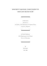
Figure 1. Steps applied to the input matrix in an iteration of the LU
factorization; Green: Just finished; Red & Orange: being processed;
Gray: Finished in previous iterations
Figure 1 presents the diagram of the basic operations applied
to the input matrix to perform the factorization. The block LU
factorization algorithm can be seen as a recursive process. At each
iteration, the panel factorization is applied on a block column. This
panel operation factorizes the upper square (selecting adequate
pivots and applying internal row swapping as necessary to ensure
numerical stability), and scales the lower polygon accordingly. The
output of this panel is used to apply row swapping to the result
of previous iterations, on the left, and to the trailing matrix on the
right. The triangular solver is applied to the right of the factored
block to scale it accordingly, and then the trailing matrix is updated
by applying a matrix-matrix multiply update. Then the trailing
matrix is used as the target for the next iteration of the recursive
algorithm, until the trailing matrix is empty. Technically, each of
these basic steps is usually performed by applying a parallel Basic
Linear Algebra Subroutine (PBLAS).
The structure of the other one-sided factorizations, Cholesky
and QR, are similar with minor differences. In the case of Cholesky,
the trailing matrix update involves only the upper triangle, as the
lower left factor is not critical. For QR, the computation of pivots
and the swapping are not necessary as the QR algorithm is more
stable. Moreover, there are a significant number of applications,
like iterative refinement and algorithms for eigenvalue problems,
where the entire factorization result, including the lower part, is
needed. Therefore, a scalable and efficient protection scheme for
the lower left triangular part of the factorization result is required.
4. Protection of the Right Factor Matrix with
ABFT
In this section, we detail the ABFT approach that is used to protect
the upper triangle from failures, while considering the intricacies
of typical block cyclic distributions and failure detection delays.
4.1 Checksum Relationship
ABFT approaches are based upon the principle of keeping an invariant
bijective relationship between protective supplementary
226

locks and the original data through the execution of the algorithm,
by the application of numerical updates to the checksum. In
order to use ABFT for matrix factorization, an initial checksum is
generated before the actual computation starts. In future references
we use G to refer to the generator matrix, and A to the original
input matrix. The checksum C for A is produced by
C = GA or C = AG (1)
When G is all-1 vector, the checksum is simply the sum of all
data items from a certain row or column. Referred to as the checksum
relationship, (1) can be used at any step of the computation for
checking data integrity (by detecting mismatching checksum and
data) and recovery (inverting the relation builds the difference between
the original and the degraded dataset). With the type of failures
we consider (Fail-Stop), data cannot be corrupted, so we will
use this relationship to implement the recovery mechanism only.
This relationship has been shown separately for Cholesky [18], and
HPL [12], both sharing the property of updating the trailing matrix
with a lower triangular matrix. However, in this work we consider
the general case of matrix factorization algorithms, including those
where the full matrix is used for trailing matrix updates (as is the
case for QR and LU with partial pivoting). In this context, the invariant
property has not been demonstrated; we will now demonstrate
that it holds for full matrix based updates algorithms as well.
4.2 Checksum Invariant with Full Matrix Update
In [22], ZU is used to represent a matrix factorization (optionally
with pairwise pivoting for LU), where Z is the left matrix (lower
triangular in the case of Cholesky or full for LU and QR) and U is
an upper triangular matrix. The factorization is then regarded as the
process of applying a series of matrices Z i to A from the left until
Z iZ i 1 ···Z 0A becomes upper triangular.
Theorem 4.1. Checksum relationship established before ZU factorization
is maintained during and after factorization.
Proof. Suppose data matrix A 2 R n⇥n is to be factored as A =
ZU, where ZandU2 R n⇥n and U is an upper triangular matrix.
A is checkpointed using generator matrix G 2 R n⇥nc , where nc
is the width of checksum. To factor A into upper triangular form,
a series of transformation matrices Z i is applied to A (with partial
pivoting in LU).
Case 1: No Pivoting
U = Z nZ n 1 ...Z 1A (2)
Now the same operation is applied to A c =[A, AG]
U c = Z nZ n 1 ...Z 1 [A, AG]
= [Z nZ n 1 ...Z 1A, Z nZ n 1 ...Z 1AG]
= [U, UG] (3)
For any k apple n, using U k to represent the result of U at step k,
Uc k = Z k Z k 1 ...Z 1 [A, AG]
= [Z k Z k 1 ...Z 1A, Z k Z k 1 ...Z 1AG]
h i
= U k , U k G
(4)
Case 2: With partial pivoting:
Uc k = Z k P k Z k 1 P k 1 ...Z 1P 1 [A, AG]
= [Z k P k Z k 1 P k 1 ...Z 1P 1A,
h
Z k P k Z k
i
1 P k 1 ...Z 1P 1AG]
= U k , U k G
(5)
Therefore the checksum relationship holds for LU with partial
pivoting, Cholesky and QR factorizations.
4.3 Checksum Invariant in Block Algorithms
Theorem 4.1 shows the mathematical checksum relationship in
matrix factorizations. However, in real-world, HPC factorizations
are performed in block algorithms, and execution is carried out
in a recursive way. Linear algebra packages, like ScaLAPACK,
consist of several function components for each factorization. For
instance, LU has a panel factorization, a triangular solver and a
matrix-matrix multiplication. We need to ensure that the checksum
relationship also holds for block algorithms, both at the end of each
iteration, and after the factorization is completed.
Theorem 4.2. For ZU factorization in block algorithm, checksum
at the end of each iteration only covers the upper triangular part of
data that has already been factored and are still being factored in
the trailing matrix.
Proof. Input Matrix A is split into blocks of data of size nb ⇥ nb
(A ij, Z ij, U ij), and the following stands:
apple apple apple
A11 A 12 A 13 Z11 Z
=
12 U11 U 12 U 13
, (6)
A 21 A 22 A 23 Z 21 Z 22 0 U 22 U 23
where A 13 = A 11 + A 12, and A 23 = A 21 + A 22.
Since A 13 = Z 11U 13 +Z 12U 23, and A 23 = Z 21U 13 +Z 22U 23,
and using the relation
8
><
>:
A 11 = Z 11U 11
A 12 = Z 11U 12 + Z 12U 22
A 21 = Z 21U 11
A 22 = Z 21U 12 + Z 22U 22
in (6), we have the following system of equations:
⇢
Z21(U 11 + U 12 U 13) =Z 22(U 23 U 22)
Z 11(U 11 + U 12 U 13) =Z 12(U 23 U 22)
This can be written as:
apple apple
Z11 Z 12 U11 + U 12 U 13
Z 21 Z 22 (U 23 U 22)
apple
Z11 Z
For LU, Cholesky and QR,
12
apple
U11 + U 12 U 13
=0
is always nonsingular, so
Z 21 Z
⇢ 22
U11 + U 12 = U 13
.
U 23 = U 22
=0, and
U 23 U 22
This shows that after ZU factorization, checksum blocks cover
the upper triangular matrix U only, even for the diagonal blocks. At
the end of each iteration, for example the first iteration in (6), Z 11,
U 11, Z 21 and U 12 are completed, and U 13 is already U 11 + U 12.
The trailing matrix A 22 is updated with
and A 23 is updated to
A 23
0
A 22 0 = A 22 Z 21U 12 = Z 22U 22.
= A 23 Z 21U 13
= A 21 + A 22 Z 21(U 11 + U 12)
= Z 21U 11 + A 22 Z 21U 11 Z 21U 12
= A 22 Z 21U 12 = Z 22U 22
Therefore, at the end of each iteration, data blocks that have already
been and are still being factored remain covered by checksum
blocks.
227

&
"
&
"
& " # &
!"" !"# !"$ !"%
!#" !## !#$ !#%
!$" !$# !$$ !$%
!%" !%# !%$ !%%
&
"
& "
!"" !"%
!$" !$%
!#" !#%
!%" !%%
!"#
!$#
!##
!%#
'()*+(,-./0 1)2+(,-./0
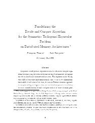
Figure 2. Example of a 2D block-cyclic data distribution
4.4 Issues with Two-Dimensional Block-cyclic Distribution
It has been well established that data layout plays an important
role in the performance of parallel matrix operations on distributed
memory systems [11, 20]. In 2D block-cyclic distributions, data
is divided into equally sized blocks, and all computing units are
organized into a virtual two-dimension grid P by Q. Each data
block is distributed to computing units in round robin following
the two dimensions of the virtual grid. Figure 2 is an example of a
P =2,Q=3grid applied to a global matrix of 4 ⇥ 4 blocks. The
same color represents the same process while numbering in A ij
indicates the location in the global matrix. This layout helps with
load balancing and reduces data communication frequency, because
in each step of the algorithm, many computing units can be engaged
in computations concurrently, and communications pertaining
to blocks positioned on the same unit can be grouped. Thanks to
these advantages, many prominent software libraries (like ScaLA-
PACK [13]) assume a 2D block-cyclic distribution.
"
!
"
!
"
" ! # "
!
# " ! #
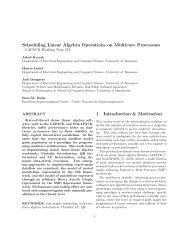
Figure 3. Holes in a checksum protected matrix caused by a single
failure and the naive checksum duplication protection scheme (3x2
process grid)
However, with a 2D block-cyclic data distribution, the failure of
a single process, usually a computing node which keeps several
non-contiguous blocks of the matrix, results in holes scattered
across the whole matrix. Figure 3 is an example of a 5 ⇥ 5 blocks
matrix (on the left) with a 2 ⇥ 3 process grid. Red blocks represent
holes caused by the failure of the single process (1, 0). In the
general case, these holes can impact both checksum and matrix data
at the same time.
4.5 Checksum Protection Against Failure
Our algorithm works under the assumption that any process can
fail and therefore the data, including the checksum, can be lost.
Rather than forcing checksum and data on different processes and
assuming only one would be lost, as in [12], we put checksum
and data together in the process grid and design the checksum
protection algorithm accordingly.
4.5.1 Minimum Checksum Amount for Block Cyclic
Distributions
Theoretically, the sum-based checksum C k of a series of N blocks
A i, 1 apple i apple N, where N is the total number of blocks in one
#
!"$
!$$
!#$
!%$
row/column of the matrix, is computed by:
NX
C k = A k (7)
k=1
With the 2D block-cyclic distribution, a single failure punches
multiple holes in the global matrix. With more than one hole per
row/column, C k in (7) is not sufficient to recover all lost data. A
slightly more sophisticated checksum scheme is required.
Theorem 4.3. Using sum-based checkpointing, for N data items
distributed in block-cyclic onto Q processes, the size of the checksum
to recover from the loss of one process is d N e Q
Proof. With 2D block-cyclic, each process gets d N e items. At the
Q
failure of one process, all data items in the group held by the
process are lost. Take data item a i, 1 apple i apple d N e, from group
Q
k, 1 apple k apple Q. To be able to recover a i, any data item in group k
cannot be used, so at least one item from another group is required
to create the checksum, and this generates one additional checksum
item. Therefore for all items in group k, d N e checksum items are
Q
generated so that any item in group k can be recovered.
Applying this theorem, we have the following checksum algorithm:
Suppose Q processes are in a process column or row, and let
each process have K blocks of data of size nb ⇥ nb. Without loss
of generality, let K be the largest number of blocks owned by any
of the Q processes. From Theorem 4.3, the size of the checksum in
this row is K blocks.
Let C i be the i th checksum item, and A j i , be the ith data item
on process j, 1 apple i appled N e, 1 apple j apple Q:
Q
QX
C k = A k k (8)
k=1
Under (8), we have the following corollary:
Corollary 4.4. The i th block of checksum is calculated using the
i th block of data of each process having at least i blocks.
4.5.2 Checksum Duplicates
Since ABFT checksum is stored by regular processors, it has to
be considered as fragile as the matrix data. From Theorem 4.3 and
using the same N and Q, the total number of checksum blocks is
K = d N e. These checksum blocks can be appended to the bottom
or to the right of the global data matrix accordingly, and since
Q
checksum is stored on computing processes, these K checksum
blocks are distributed over min (K, Q) processes (see Figure 3).
If a failure strikes any of these processes, like (1, 0) in this example,
some checksum is lost and cannot be recovered. Therefore,
checksum itself needs protection; in our work, duplication is used
to protect checksum from failure.
A straightforward way of performing duplication is to make
a copy of the entire checksum block, as illustrated by the two
rightmost columns in Figure 3. While simple to implement, this
method suffers from two major defects. First, if the checksum
width K is a multiple of Q (or P for column checksum), the
duplicate of a checksum block is located on the same processors,
defeating the purpose of duplication. This can be solved at the cost
of introducing an extra empty column in the process grid to resolve
the mapping conflict. More importantly, to maintain the checksum
invariant property, it is required to apply the trailing matrix update
on the checksum (and its duplicates) as well. From corollary 4.4,
once all the i th block columns on each process have finished the
panel factorization (in Q step), the i th checksum block column is
no longer active in any further computation (except pivoting) and
228

should be excluded from the computing scope to reduce the ABFT
overhead. This is problematic, as splitting the PBLAS calls to avoid
excluded columns has a significant impact on the trailing matrix
update efficiency.
4.5.3 Reverse Neighboring Checksum Storage
With the observation of how checksum is maintained during factorization,
we propose the following reverse neighboring checksum
duplication method that allows for applying the update in a single
PBLAS call without incurring extraneous computation.
Algorithm 1 Checksum Management
On a P ⇥ Q grid, matrix is M ⇥ N, block size is NB ⇥ NB
C k represents the k th checksum block column
A k represents the k th data block column
Before factorization:
Generate the initial checksum:
C k = P l m
(k 1)⇥Q+Q
j=(k 1)⇥Q+1 Aj, k =1, ··· , N
NB⇥Q
For each of C k , make a copy of the whole block column and put
right next to its original block column
Checksum C k and its copy are put in the k th position starting
from the far right end
Begin factorization
Host l malgorithm starts with an initial scope of M rows and
N + columns
N
Q
For each Q panel factorizations, the scope decreases M rows
and 2 ⇥ NB columns
End factorization
two last block columns of checksum are excluded from the TRSM
and GEMM scope. Since TRSM and GEMM claim most of the
computation in the LU factorization, this shrinking scope greatly
reduces the overhead of the ABFT mechanism. One can note that
only the upper part of the checksum is useful, we will explain in the
next section how this extra storage can be used to protect the lower
triangular part of the matrix.
4.6 Delayed Recovery and Error Propagation
In this work, we assume that a failure can strike at any moment
during the life span of factorization operations or even the recovery
process. Theorem 4.2 proves that at the moment where the failure
happens, the checksum invariant property is satisfied, meaning that
the recovery can proceed successfully. However, in large scale systems,
which are asynchronous by nature, the time interval between
the failure and the moment when it is detected by other processes
is unknown, leading to delayed recoveries, with opportunities for
error propagation.
The ZU factorization is composed of several sub-algorithms
that are called on different parts of the matrix. Matrix multiplication,
which is used for trailing matrix updates and claims more than
95% of the execution time, has been shown to be ABFT compatible
[4] , that is to compute the correct result even with delayed
recovery. One feature that has the potential to curb this compatibility
is pivoting, in LU, especially when a failure occurs between
the panel factorization and the row swapping updates, there is a
potential for destruction of rows in otherwise unaffected blocks.
! " # ! " # ! "
# ! " # ! "
!
"
!
"
!
"
!
"
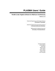
Figure 4. Reverse neighboring checksum storage, with two checksum
duplicates per Q-wide groups
Figure 4 is an example of the reverse neighboring checksum
method on a 2⇥3 grid. The data matrix has 8⇥8 blocks and therefore
the size of checksum is 8 ⇥ 3 blocks with an extra 8 ⇥ 3 blocks
copy. The arrows indicate where checksum blocks are stored on the
right of the data matrix, according to the reverse storage scheme.
For example, in the LU factorization, the first 3 block columns produce
the checksum in the last two block columns (hence making
2 duplicate copies of the checksum). Because copies are stored
in consecutive columns of the process grid, for any 2D grid with
Q>1, the checksum duplicates are guaranteed to be stored on different
processors. The triangular solve (TRSM) and trailing matrix
update (GEMM) are applied to the whole checksum area until the
first three columns are factored. In following factorization steps, the
Figure 5. Ghost pivoting Issue
Gray: Result in previous steps
Light Green: Panel factorization result in current step
Deep Green: The checksum that protects the light green
Blue: TRSM zone Yellow: GEMM zone
Red: one of the columns affected by pivoting
Figure 5 shows an example of such a case. Suppose the current
panel contributes to the i th column of checksum. When panel
factorization finishes, the i th column becomes intermediate data
which does not cover any column of matrix. If a failure at this
instant causes holes in the current panel area, then lost data can
be recovered right away. Pivoting for this panel factorization has
only been applied within the light green area. Panel factorization
is repeated to continue on the rest of the factorization. However, if
failure causes holes in other columns that also contribute to the
i th column of checksum, these holes cannot be recovered until
the end of the trailing matrix update. To make it worse, after the
panel factorization, pivoting starts to be applied outside the panel
area and can move rows in holes into healthy area or vice versa,
229

extending the recovery area to the whole column, as shown in red
in Figure 5 including triangular solving area. To recover from this
case, in addition to matrix multiplication, the triangular solver is
also required to be protected by ABFT.
Theorem 4.5. Failure in the right-hand sides of triangular solver
can recover from fail-stop failure using ABFT.
Proof. Suppose A is the upper or lower triangular matrix produced
by LU factorization (non-blocked in ScaLAPACK LU), B is the
right-hand side, and the triangular solver solves the equation Ax =
B.
Supplement B with checksum generated by B c = B ⇤ G r to
extended form ˆB =[B, B c], where G r is the generator matrix.
Solve the extended triangular equation:
Ax c = B c =[B, B c]
) x c = A 1 ⇥ [B, B c]
= ⇥ A 1 B, A 1 ⇤
B c
= ⇥ x, A 1 ⇤
BG r
= [x, xG r]
Therefore data in the right-hand sides of the triangular solver is
protected by ABFT.
With this theorem, if failure occurs during triangular solving,
lost data can be recovered when the triangular solver completes.
Since matrix multiplication is also ABFT compatible, the whole red
region in Figure 5 can be recovered after the entire trailing matrix
update is done, leaving the opportunity for failure detection and
recovery to be delayed at a convenient moment in the algorithm.
PBLAS kernel used to compute the panel factorization (see Figure
1) performs simultaneously the search for the best pivot in the
column and the scaling of the column with that particular pivot. If
applied directly on the matrix and the checksum blocks, similarly to
what the trailing update approach does, checksum elements are at
risk of being selected as pivots, which results in exchanging checksum
rows into the matrix. This difficulty could be circumvented by
introducing a new PBLAS kernel that does not search for pivots in
the checksum.
Unfortunately, legitimate pivoting would still break the checksum
invariant property, due to row swapping. In LU, for matrix A,
A =
=
✓ ◆ ✓ ◆✓ ◆
A11 A 12 L11 0 U11 U
=
12
A 21 A 22 L 21 L 22 0 U 22
✓ ◆
L11U 11 L 11U 12
(9)
L 21U 11 L 21U 12 + L 22U 22
Panel factorization is:
✓
A11
A 21
◆
=
✓
L11U 11
L 21U 11
◆
=
✓
L11
L 21
◆
U 11 (10)
To protect L 11 and L 21, imagine that we maintain a separate
checksum, stored at the bottom of the matrix, as shown in the
yellow bottom rectangle of Figure 6, that we plan on updating
by scaling it accordingly to the panel operation. In this vertical
checksum, each P tall group of blocks in the 2D block cyclic
distribution is protected by a particular checksum block. Suppose
rows i 1 and i 2 reside on blocks k i1 and k j1 of two processes.
It is not unusual that k i1 6= k j1 . By Corollary 4.4, block k i1
and k j1 contribute to column-wise checksum block k i1 and k j1
respectively in the column that local blocks k i1 and k j1 belong to.
This relationship is expressed as
row i 1
7! checksum block k i1
row j 1
7! checksum block k j1
7! reads ’contributes to’. After the swapping, the relationship
should be updated to
Figure 6. Separation of lower and upper areas protected by checksum
(green) and checkpoint (yellow) during the course of the factorization
algorithm
5. Protection of the Left Factor Matrix with
Q-parallel Checkpoint
It has been proven in Theorem 4.2 that the checksum only covers
the upper triangular part of the matrix until the current panel, and
the trailing matrix is subject to future updates. This is depicted in
Figure 6, where the green checksum on the right of the matrix protects
exclusively the green part of the matrix. Another mechanism
must be added for the protection of the left factor (the yellow area).
5.1 Impracticability of ABFT for Left Factor Protection
The most straightforward idea, when considering the need of protecting
the lower triangle of the matrix, is to use an approach similar
to the one described above, but column-wise. Unfortunately, such
an approach is difficult, if not impossible in some cases, as proved
in the remaining of this Section.
5.1.1 Pivoting and Vertical Checksum Validity
In LU, partial pivoting prevents the left factor from being protected
through ABFT. The most immediate reason is as follow: The
row i 1 7! checksum block k j1
row j 1 7! checksum block k i1
This requires a re-generation of checksum blocks k i1 and k j1 in
order to maintain the checkpoint validity. Considering there are nb
potential pivoting operations per panel, hence a maximum of nb+1
checksum blocks to discard, this operation has the potential to be
as expensive as computing a complete vertical checkpoint.
5.1.2 QR Factorization
Although QR has no pivoting, it still cannot benefit from ABFT to
cover Q, as we prove below.
Theorem 5.1. Q in Householder QR factorization cannot be protected
by performing factorization along with the vertical checksum.
Proof. Append a m ⇥ n nonsingular matrix A with checksum apple GA
A
of size c⇥n along the column direction to get matrix A c =
GA .
G is c ⇥ m generator matrix. Suppose A has a QR factorization
Q 0R 0.
Perform QR factorization to A c:
apple apple apple
A
GA = QcRc = Qc11 Q c12 Rc11
Q c21 Q c22 ?
230

Q c11 is m ⇥ m and Q c21 is c ⇥ m. R c is m ⇥ n and ? represents
c ⇥ n zero matrix. R c 6= 0and is full rank. Because R c is upper
triangular with nonzero diagonal elements and therefore nonsingular.
Therefore
Q cQ T c =
apple
Qc11
Q c12
Q c21 Q c22
apple
Q
T
c11 Q T c21
Q T c12
Q T c22
= I
Q c11Q T c11 + Q c12Q T c12 = I. (11)
Since A = Q c11R c11 and R c11 is nonsingular, then Q c11 6= 0and
nonsingular.
Assume Q c12 =0:
Q c11Q T c21 + Q c12Q T c22 =0, therefore Q c11Q T c21 =0. We have
shown that Q c11 is nonsingular, so Q T c21 = 0 and this conflicts
with GA = Q c21R c11 6= 0, so the assumption Q c12 =0does not
hold. From Equation 11, Q c11Q T c11 6= I. This means even though
A = Q c11R c11, Q c11R c11 is not a QR factorization of A.
5.2 Panel Checkpointing
Given that the ZU factorization cannot protect Z by applying
ABFT in the same way as for U, separate efforts are needed.
For the rest of this paper, we use the term “checksum” to refer
to the ABFT checksum, generated before the factorization, that
is maintained by the application of numerical updates during the
course of the algorithm, in contrast to “checkpointing” for the
operation that creates a new protection block during the course
of the factorization. LU factorization with partial pivoting being
the most complex problem, it is used here for the discussion. The
method proposed in this section can be applied to the QR and
Cholesky factorizations with minimal efforts nonetheless.
In a ZU block factorization using 2D cyclic distribution, once a
panel of Z is generated, it is stored into the lower triangular region
of the original matrix. For example, in LU, vectors of L, except the
diagonal ones, are stored in L. These lower triangular parts from the
panel factorization are final results, and are not subject to further
updates during the course of the algorithm, except for partial pivoting
row swapping in LU. Therefore only one vertical checkpointing
“should be” necessary to maintain each panel’s safety, as is discussed
in [12]. We will show how this idea, while mathematically
trivial, needs to be refined to support partial pivoting. We will then
propose a novel checkpointing scheme, leveraging properties of the
block algorithm to checkpoint Z in parallel, that demonstrates a
much lower overhead when compared to this basic approach.
5.3 Postponed Left Pivoting
Although once a panel is factored, it is not changed until the end
of the computation, row swaps incurred by pivoting are still to
be applied to the left factor as the algorithm progresses in the
trailing matrix, as illustrated in Figure 1. The second step (pivoting
to the left) swaps two rows to the left of the current panel. The
same reasoning as presented in section 5.1.1 holds, meaning that
the application of pivoting row swaps to the left factor has the
potential to invalidate checkpoint blocks. Since pivoting to the left
is carried out in every step of LU, this causes significant checkpoint
maintenance overhead.
Unlike pivoting to the right, which happens during updates and
inside the panel operation, whose result are reused in following
steps of the algorithm, pivoting to the left can be postponed. The
factored L is stored in the lower triangular part of the matrix
without further usage during the algorithm. As a consequence,
we delay the application of all left pivoting to the end of the
computation, in order to avoid expensive checkpoint management.
We keep track of all pivoting that should have been applied to the
left factor, and when the algorithm has completed, all row swaps are
applied just in time before returning the end-result of the routine.
5.4 Q-Parallel Checkpointing of Z
The vertical checkpointing of the panel result requires a set of
reduction operations immediately after each panel factorization.
Panel factorization is on the critical path and has lower parallelism,
compared to other routines of the factorization (such as trailing
matrix update). The panel factorization works only on a single
block column of the matrix, hence benefits from only a P degree of
parallelism, in a P ⇥ Q process grid. Checkpointing worsens this
situation, because it applies to the same block column, and is bound
to the same low level of exploitable parallelism. Furthermore, the
checkpointing cannot be overlapped with the computation of the
trailing matrix update: all processes who do not appear on the
same column of the process grid are waiting in the matrix-matrix
multiply PBLAS, stalled because they require the panel column to
enter the call in order for the result of the panel to be broadcasted. If
the algorithm enters the checkpointing routine before going into the
trailing update routine, the entire update is delayed. If the algorithm
enters the trailing update before starting the checkpointing, the
checksum is damaged in a way that prevents recovering that panel,
leaving it vulnerable to failures.
Our proposition is then twofold: we protect the content of the
blocks before the panel, which then enables starting immediately
the trailing update without jeopardizing the safety of the panel
result. Then, we wait until sufficient checkpointing is pending to
benefit from the maximal parallelism allowed by the process grid.
5.4.1 Enabling Trailing Matrix Update Before Checkpointing
The major problem with enabling the trailing matrix update to proceed
while the checkpointing of the panel is not finished is that the
ABFT protection of the update modifies the checksum in a way that
disables protection for the panel blocks. To circumvent this limitation,
in a P ⇥ Q grid, processes are grouped by section of width
Q, that are called a panel scope. When the panel operation starts
applying to a new section, the processes of this panel scope make
a local copy of the impending column and the associated checksum,
called a snapshot. This operation involves no communication,
and features the maximum P ⇥ Q parallelism. The memory overhead
is limited, as it requires only the space for at most two extra
columns to be available at all time, one for saving the state before
the application of the panel to the target column, and one for the
checksum column associated to these Q columns. The algorithm
then proceeds as usual, without waiting for checkpoints before entering
the next Q trailing updates. Because of the availability of this
extra protection column, the original checksum can be modified to
protect the trailing matrix without threatening the recovery of the
panel scope, which can rollback to that previous dataset should a
failure occur.
5.4.2 Q-Parallel Checkpointing
When a panel scope is completed, the P ⇥Q group of processes undergo
checkpointing simultaneously. Effectively, P simultaneous
checkpointing reductions are taking place along the block rows,
involving the Q processes of that row to generate a new protection
block. This scheme enables the maximum parallelism for the
checkpoint operation, hence decreasing its global impact on the
failure free overhead. Another strong benefit is that it scales with
the process grid perfectly, whereas regular checkpointing suffers
from scaling with the square root of the number of processes (as it
involves only one dimension of the process grid).
231

!"#$%&'
()*+,-./'
!"#$%&'
0' 1'
(' 2'
Figure 7. Recovery example
(matrix size 800 ⇥ 800, grid size 2 ⇥ 3, failure of process (0,1), failure step:41,
A: Failure occurs B: Checksum recovered
C: Data recovered using ABFT checksum and checkpointing output D: Three panels restored using snapshots
5.4.3 Optimized Checkpoint Storage
According to Corollary 4.4, starting from the first block column on
the left, every Q block columns contribute to one block column
of checksum, which means that once the factorization is done
for these Q block columns, the corresponding checksum block
column becomes useless (it does not protect the trailing matrix
anymore, it has never protected the left factor, see Theorem 4.2).
Therefore, this checksum storage space is available for storing the
resultant checkpoint block generated to protect the panel result.
Following the same policy as the checksum storage, discussed in
Section 4.5.2, the checkpoint data is stored in reverse order from the
right of the checksum (see Figure 4). As this part of the checksum
is excluded from the trailing matrix update, the checkpoint blocks
are not modified by the continued operation of the algorithm.
5.4.4 Recovery
The hybrid checkpointing approach requires a special recovery algorithm.
Two cases are considered. First, when failure strikes during
the trailing update, immediately after a panel scope checkpointing.
For this case, the recovery is not attempted until the current
step of the trailing update is done. When the recovery time comes,
the checksum/checkpointing on the right of the matrix matches the
matrix data as if the initial ABFT checksum had just been performed.
Therefore any lost data blocks can be recovered by the
simple reverse application of the ABFT checksum relationship.
The second case is when a failure occurs during the Q panel
factorization, before the checkpointing for this panel scope can
successfully finish. In this situation, all processes revert the panel
scope columns to the snapshot copy. Holes in the snapshot data are
recreated by using the snapshot copy of the checksum, applying the
usual ABFT recovery. The algorithm is resumed in the panel scope,
so that panel and updates are applied again within the scope of the
Q wide section; updates outside the panel scope are discarded, until
the pre-failure iteration has been reached. Outside the panel scope,
regular recovery mechanisms are deployed (ABFT checksum inversion
for the trailing matrix, checkpoint recovery for the left factor).
When the re-factorization of panels finishes, the entire matrix, including
the checksum, is recovered back to the correct state. The
computation then resumes from the next panel factorization, after
the failing step.
Figure 7 shows an example of the recovery when the process
(1,0) in a 2 ⇥ 3 grid failed. It presents the difference between
the correct matrix dataset and the current dataset during various
steps of failure recovery as a “temperature map”, brighter colors
meaning large differences and black insignificant differences. The
matrix size is 80 ⇥ 80 and NB =10, therefore the checksum size
is 80 ⇥ 60. Failure occurs after the panel factorization starting at
(41,41) is completed, within the Q =3panel scope. First, using
a fault tolerant MPI infrastructures, like FT-MPI [15], the failed
process (0,1) is replaced and reintegrates the process grid with a
blank dataset, showing as evenly distributed erroneous blocks (A).
Then the recovery process starts by mending the checksum using
duplicates (B). The next step recovers the data which is outside
the current panel scope (31:80,31:60), using the corresponding
checksum for the right factor, and the checkpoints for the left factor
(C). At this moment, all the erroneous blocks are repaired, except
those in the panel scope (41:80, 41:50). Snapshots are applied to
the three columns of the panel scope (31:80,31:60). Since these do
not match the state of the matrix before the failure, but a previous
state, this area appears as very different (D). Panel factorization
is re-launched in the panel scope, in the area (31:80,31:60), with
the trailing update limited within this area. This re-factorization
continues until it finishes panel (41:80,41:50) and by that time the
whole matrix is recovered to the correct state (not presented, all
black). The LU factorization can then proceed normally.
6. Evaluation
In this section, we evaluate the performance of the proposed fault
tolerant algorithm based on ABFT and reverse neighboring checkpointing.
For a fault tolerant algorithm, the most important consid-
232

./012$34567589:;4$%/($ B7:0./$12$34567589:;4$%/($ /$7C45D49E$%F($
1)*2#*3,45)&.!"#$6%0&
&"$
@"$
)"$
,"$
!"$
*"$
"$
!"#$%&'&($ )"#$%*!'*!($ +"#$%!)'!)($ *&"#$%)+')+($ ,!"#$%-&'-&($ &)"#$%*-!'*-!($
./012$34567589:;4$%/($ "?*)!,&**)$ "?@&+@&A!&-$ !?!*"-&,A+!$ &?+&+-+"+"+$ !"?@A,,!*"&$ )+?+-+&-@,*$
B7:0./$12$34567589:;4$%/($ "?*-!-"-,A$ "?&,)!@+*)A$ !?!+",&A)+*$ &?+-"!&-@-*$ !"?@-*"!!)-$ )+?-"&@"A@+$
/$7C45D49E$%F($ !&?!","-A,,$ *"?,@A**---$ ,?"),@,*,)!$ "?,"+-&++",$ "?"+@-&&A!+$ "?"*@-A,+A*$
!"#$%&'()*+),-&./0&
3,7*89&%8:)&.;*8-&%8:)0&
Figure 8. Weak scalability of FT-LU: performance and overhead
on Kraken, compared to non fault tolerant LU
FT overhead (Tflop/s) 0.051 0.066 0.070 0.021 0.018 0.008
FT overhead (%) 26.203 10.357 3.044 0.309 0.086 0.016
eration is the overhead added to failure free execution rate, due to
various fault tolerance mechanisms such as checksum generation,
checkpointing and extra flops. An efficient and scalable algorithm
will incur a minimal overhead over the original algorithm while
enabling scalable reconstruction of lost dataset in case of failure.
We use the NSF Kraken supercomputer, hosted at the National
Institute for Computational Science (NICS, Oak Ridge, TN) as
our testing platform. This machine features 112,896 2.6GHz AMD
Opteron cores, 12 cores per node, with the Seastar interconnect. At
the software level, to serve as a comparison base, we use the non
fault tolerant ScaLAPACK LU and QR in double precision with
block size NB = 100. The fault tolerance functions are implemented
and inserted as drop-in replacements for ScaLAPACK routines.
In this section, we first evaluate the storage overhead in the form
of extra memory usage, then show experimental result on Kraken
to assess the computational overhead.
6.1 Storage Overhead
Checksum takes extra storage (memory), but on large scale systems,
memory usage is usually maximized for computing tasks.
Therefore, it is preferable to have a small ratio of checksum size
over matrix size, in order to minimize the impact on the memory
available to the application itself. For the sake of simplicity, and
because of the small impact in term of memory usage, neither the
pivoting vector nor the column shift are considered in this evaluation.
Different protection algorithms require different amounts of
memory. In the following, we consider the duplication algorithm
presented in Section 4.5.2 for computing the upper memory bound.
The storage of the checksum includes the row-wise and columnwise
checksums and a small portion at the bottom-right corner.
For an input matrix of size M ⇥ N on a P ⇥ Q process grid, the
memory used for checksum (including duplicates) is M ⇥ N ⇥ 2. Q
The ratio R mem of checksum memory over the memory of the
input matrix, equals to 2 , becomes negligible with the increase
Q
in the number of processes used for the computation.
6.2 Overhead without Failures
Figure 8 evaluates the completion time overhead and performance,
using the LU factorization routine PDGETRF. The performance of
both the original and fault tolerant version are presented, in Tflop/s
,"$
!@$
!"$
*@$
*"$
@$
"$
!"#$%&'$()'*+',-$./0$
#!"
'#"
'!"
&#"
&!"
%#"
%!"
$#"
$!"
#"
!"
./01234"56"7"8/6419":53;43"
./01234"06"7"8/6419"
?5"43353"
%!(")*+*," '!(")$%+$%," -!(")%'+%'," $*!(")'-+'-,"
1,2*34$536'$.7*3-$536'0$
Figure 9. Weak scalability of FT-LU: run time overhead on
Kraken when failures strike at different steps
(the two curves overlap due to the little performance difference).
This experiment is carried out to test the weak scalability, where
both the matrix and grid dimension doubles. The result outlines
that as the problem size and grid size increases, the overhead drops
quickly and eventually becomes negligible. At the matrix size of
640, 000 ⇥ 640, 000, on 36, 864 (192 ⇥ 192) cores, both versions
achieved over 48Tflop/s, with an overhead of 0.016% for the ABFT
algorithm. As a side experiment, we implemented the naive vertical
checkpointing method discussed in section 5.2, and as expected the
measured overhead quickly exceeds 100%.
As the left factor is touched only once during the computation,
the approach of checkpointing the result of a panel synchronously
can, a-priori, look sound when compared to system based checkpoint,
where the entire dataset is checkpointed periodically. However,
as the checkpointing of a particular panel suffers from its inability
to exploit the full parallelism of the platform, it is subject to
a derivative of Amdahl’s law, its parallel efficiency is bound by P,
while the overall computation enjoys a P ⇥ Q parallel efficiency:
its importance is bound to grow when the number of computing resources
increases. As a consequence, in the experiments, the time
to compute the naive checkpoint dominates the computation time.
On the other hand, the hybrid checkpointing approach exchanges
the risk of a Q-step rollback with the opportunity to benefit from
a P ⇥ Q parallel efficiency for the panel checkpointing. Because
of this improved parallel efficiency, the hybrid checkpointing approach
benefits from a competitive level of performance, that follows
the same trend as the original non fault tolerant algorithm.
6.3 Recovery Cost
In addition to the “curb” overhead of fault tolerance functions, the
recovery from failure adds extra overhead to the host algorithm.
There are two cases for the recovery. The first one is when failure
occurs right after the reverse neighboring checkpointing of Q panels.
At this moment the matrix is well protected by the checksum
and therefore the lost data can be recovered directly from the checksum.
We refer to this case as “failure on Q panels border”. The second
case is when the failure occurs during the reverse neighboring
checkpointing and therefore local snapshots have to be used along
with re-factorization to recover the lost data and restore the matrix
state. This is referred to as the ”failure within Q panels”.
Figure 9 shows the overhead from these two cases for the LU
factorization, along with the no-error overhead as a reference. In
the “border” case, the failure is simulated to strike when the 96 th
panel (which is a multiple of grid columns, 6, 12, ··· , 48) has
233

!"#$%&'$()'*+',-$./0$
'#"
'!"
&#"
&!"
%#"
%!"
$#"
$!"
#"
!"
./"0123"45678549"
./"0123":7"54474"
%!(")*+*," '!(")$%+$%," -!(")%'+%'," $*!(")'-+'-,"
1,2*34$536'$.7*3-$536'0$
Figure 10. Weak scalability of FT-QR: run time overhead on
Kraken when failures strike
just finished. In the “non-border” case, failure occurs during the
(Q +2) th panel factorization. For example, when Q =12, the
failure is injected when the trailing update for the step with panel
(1301,1301) finishes. From the result in Figure 9, the recovery
procedure in both cases adds a small overhead that also decreases
when scaled to large problem size and process grid. For largest
setups, only 2-3 percent of the execution time is spent recovering
from a failure.
6.4 Extension to Other factorization
The algorithm proposed in this work can be applied to a wide range
of dense matrix factorizations other than LU. As a demonstration
we have extended the fault tolerance functions to the ScaLAPACK
QR factorization in double precision. Since QR uses a block algorithm
similar to LU (and also similar to Cholesky), the integration
of fault tolerance functions is mostly straightforward. Figure 10
shows the performance of QR with and without recovery. The overhead
drops as the problem and grid size increase, although it remains
higher than that of LU for the same problem size. This is
expected: as the QR algorithm has a higher complexity than LU
( 4 N 3 v.s. 2 N 3 ), the ABFT approach incurs more extra computation
when updating checksums. Similar to the LU result, recovery
3 3
adds an extra 2% overhead. At size 160,000 a failure incurs about
5.7% penalty to be recovered. This overhead becomes lower, the
larger the problem or processor grid size considered.
7. Conclusion
In this paper, by assuming a failure model in which fail-stop failures
can occur anytime on any process during a parallel execution, a
general scheme of ABFT algorithms for protecting one-sided matrix
factorizations is proposed. This scheme can be applied to a
wide range of dense matrix factorizations, including Cholesky, LU
and QR. A significant property of the proposed algorithms is that
both the left and right factorization results are protected. ABFT is
used to protect the right factor with checksum generated before, and
carried along during the factorizations. A highly scalable checkpointing
method is proposed to protect the left factor. This method
cooperatively reutilizes the memory space originally designed to
store the ABFT checksum, and has minimal overhead by strategically
coalescing checkpoints of many iterations. Large scale experimental
results validate the design of the proposed fault tolerance
method by highlighting scalable performance and decreasing overhead
for both LU and QR. In the future this work will be extended
to support multiple simultaneous failures.
References
[1] Fault tolerance for extreme-scale computing workshop report, 2009.
[2] http://www.top500.org/, 2011.
[3] L. Blackford, A. Cleary, J. Choi, E. D’Azevedo, J. Demmel, I. Dhillon,
J. Dongarra, S. Hammarling, G. Henry, A. Petitet, et al. ScaLAPACK
users’ guide. Society for Industrial Mathematics, 1997.
[4] G. Bosilca, R. Delmas, J. Dongarra, and J. Langou. Algorithm-based
fault tolerance applied to high performance computing. Journal of
Parallel and Distributed Computing, 69(4):410–416, 2009.
[5] A. Bouteiller, G. Bosilca, and J. Dongarra. Redesigning the message
logging model for high performance. Concurrency and Computation:
Practice and Experience, 22(16):2196–2211, 2010.
[6] G. Burns, R. Daoud, and J. Vaigl. LAM: An open cluster environment
for MPI. In Proceedings of SC’94, volume 94, pages 379–386, 1994.
[7] F. Cappello. Fault tolerance in petascale/exascale systems: Current
knowledge, challenges and research opportunities. International Journal
of High Performance Computing Applications, 23(3):212, 2009.
[8] Z. Chen and J. Dongarra. Algorithm-based checkpoint-free fault
tolerance for parallel matrix computations on volatile resources. In
IPDPS’06, pages 10–pp. IEEE, 2006.
[9] Z. Chen and J. Dongarra. Scalable techniques for fault tolerant
high performance computing. PhD thesis, University of Tennessee,
Knoxville, TN, 2006.
[10] Z. Chen and J. Dongarra. Algorithm-based fault tolerance for fail-stop
failures. IEEE TPDS, 19(12):1628–1641, 2008.
[11] J. Choi, J. Demmel, I. Dhillon, J. Dongarra, S. Ostrouchov, A. Petitet,
K. Stanley, D. Walker, and R. Whaley. ScaLAPACK: a portable linear
algebra library for distributed memory computers–design issues and
performance. Computer Physics Comm., 97(1-2):1–15, 1996.
[12] T. Davies, C. Karlsson, H. Liu, C. Ding, , and Z. Chen. High Performance
Linpack Benchmark: A Fault Tolerant Implementation without
Checkpointing. In Proceedings of the 25th ACM International Conference
on Supercomputing (ICS 2011). ACM.
[13] J. Dongarra, L. Blackford, J. Choi, A. Cleary, E. D’Azevedo, J. Demmel,
I. Dhillon, S. Hammarling, G. Henry, A. Petitet, et al. ScaLA-
PACK user’s guide. Society for Industrial and Applied Mathematics,
Philadelphia, PA, 1997.
[14] E. Elnozahy, D. Johnson, and W. Zwaenepoel. The performance
of consistent checkpointing. In Reliable Distributed Systems, 1992.
Proceedings., 11th Symposium on, pages 39–47. IEEE, 1991.
[15] G. Fagg and J. Dongarra. FT-MPI: Fault tolerant MPI, supporting
dynamic applications in a dynamic world. EuroPVM/MPI, 2000.
[16] G. Gibson. Failure tolerance in petascale computers. In Journal of
Physics: Conference Series, volume 78, page 012022, 2007.
[17] G. Golub and C. Van Loan. Matrix computations. Johns Hopkins Univ
Pr, 1996.
[18] D. Hakkarinen and Z. Chen. Algorithmic Cholesky factorization fault
recovery. In Parallel & Distributed Processing (IPDPS), 2010 IEEE
International Symposium on, pages 1–10. IEEE, 2010.
[19] K. Huang and J. Abraham. Algorithm-based fault tolerance for matrix
operations. Computers, IEEE Transactions on, 100(6):518–528, 1984.
[20] V. Kumar, A. Grama, A. Gupta, and G. Karypis. Introduction to
parallel computing: design and analysis of algorithms, volume 400.
Benjamin/Cummings, 1994.
[21] C. Lu. Scalable diskless checkpointing for large parallel systems. PhD
thesis, Citeseer, 2005.
[22] F. Luk and H. Park. An analysis of algorithm-based fault tolerance
techniques* 1. Journal of Parallel and Distributed Computing,
5(2):172–184, 1988.
[23] J. Plank, K. Li, and M. Puening. Diskless checkpointing. Parallel and
Distributed Systems, IEEE Transactions on, 9(10):972–986, 1998.
[24] F. Streitz, J. Glosli, M. Patel, B. Chan, R. Yates, B. Supinski, J. Sexton,
and J. Gunnels. Simulating solidification in metals at high pressure:
The drive to petascale computing. In Journal of Physics: Conference
Series, volume 46, page 254. IOP Publishing, 2006.
234