ChemFlux Tutorial Manual - SoilVision Systems, Ltd

2D / 3D Contaminant Transport Modeling
Software
Tutorial Manual
ED-4B
Date: November 19, 2004
Written by:
Jason Stianson, B.Sc.C.E.
Robert Thode, B.Sc.G.E.
Edited by:
Murray Fredlund, Ph.D.
SoilVision Systems Ltd.
Saskatoon, Saskatchewan, Canada

Software License
The software described in this manual is furnished under a license agreement. The software may be used or
copied only in accordance with the terms of the agreement.
Software Support
Support for the software is furnished under the terms of a support agreement.
Copyright
Information contained within this Tutorial Manual is copyrighted and all rights are reserved by SoilVision
Systems Ltd. The CHEMFLUX software is a proprietary product and trade secret of SoilVision Systems. The
Tutorial Manual may be reproduced or copied in whole or in part by the software licensee for use with running
the software. The Tutorial Manual may not be reproduced or copied in any form or by any means for the
purpose of selling the copies.
Disclaimer of Warranty
SoilVision Systems Ltd. reserves the right to make periodic modifications of this product without obligation to
notify any person of such revision. SoilVision does not guarantee, warrant, or make any representation
regarding the use of, or the results of, the programs in terms of correctness, accuracy, reliability, currentness, or
otherwise; the user is expected to make the final evaluation in the context of his (her) own problems.
Trademarks
Windows is a registered trademark of Microsoft Corporation.
SoilVision is a registered trademark of SoilVision Systems Ltd.
CHEMFLUX is a trademark of SoilVision Systems Ltd.
SVFLUX is a trademark of SoilVision Systems Ltd.
FlexPDE ® is a registered trademark of PDE Solutions Inc.
Copyright © 2004
by
SoilVision Systems Ltd.
Saskatoon, Saskatchewan, Canada
ALL RIGHTS RESERVED
Printed in Canada

SoilVision Systems Ltd. Table of Contents Page 3 of 58
1 A TWO DIMENSIONAL EXAMPLE PROBLEM...................................................................... 5
1.1 STEADY-STATE SVFLUX SOLUTION ........................................................................... 5
1.2 CHEMFLUX SOLUTION DATA....................................................................................... 8
1.3 SVFLUX GRADIENTS FILE............................................................................................ 8
1.4
1.5
ADDING A CHEMFLUX PROJECT ............................................................................... 9
ADDING A CHEMFLUX PROBLEM............................................................................. 11
1.6 OPENING THE CHEMFLUX PROBLEM ..................................................................... 12
1.7 DEFINING THE CHEMFLUX PROBLEM..................................................................... 13
1.7.1 Import SVFLUX Geometry........................................................................................ 13
1.7.2 Specify Settings......................................................................................................... 15
1.7.3
1.7.4
Define Material Properties........................................................................................ 17
Assign Soils to Regions.......................................................................................... 18
1.7.5 Specify Boundary Conditions.................................................................................... 19
1.8
1.9
SPECIFY PLOTS ........................................................................................................... 20
SPECIFY OUTPUT FILES ............................................................................................ 22
1.10 ANALYZE......................................................................................................................... 23
1.11 RESULTS ........................................................................................................................ 23
2 A THREE DIMENSIONAL EXAMPLE PROBLEM................................................................ 27
2.1 STEADY STATE SVFLUX SOLUTION........................................................................ 27
2.2
2.3
CHEMFLUX SOLUTION DATA..................................................................................... 33
SVFLUX GRADIENTS FILE.......................................................................................... 34
2.4 ADDING A CHEMFLUX PROJECT ............................................................................. 34
2.5
2.6
ADDING A CHEMFLUX PROBLEM............................................................................. 36
OPENING THE PROBLEM........................................................................................... 37
2.7 DEFINING THE PROBLEM........................................................................................... 38
2.7.1 Import SVFLUX Geometry........................................................................................ 38
2.7.2 Specify Settings......................................................................................................... 39
2.7.3 Define Material Properties........................................................................................ 42
2.7.4 Specifying a Soil by Region and Layer............................................................... 44
2.7.5 Specify Boundary Conditions.................................................................................... 45
2.8 SPECIFY PLOTS ........................................................................................................... 46
2.9 SPECIFY OUTPUT FILES ............................................................................................ 48
2.10 ANALYZE......................................................................................................................... 49
2.11 RESULTS ........................................................................................................................ 49
2.11.1 Solution Mesh............................................................................................................ 50
2.11.2 Concentration Contours............................................................................................. 51
2.11.3 Flow Vectors.............................................................................................................. 52
2.11.4 AcuMesh..................................................................................................................... 52

SoilVision Systems Ltd. Table of Contents Page 4 of 58
3 REFERENCES.......................................................................................................................... 56
4 INDEX ....................................................................................................................................... 57

SoilVision Systems Ltd. A Two Dimensional Example Problem Page 5 of 58
1 A TWO DIMENSIONAL EXAMPLE PROBLEM
Sudicky (1989) developed the following example. The problem considers flow and solute transport in a
heterogeneous cross section with a highly irregular flow field, dispersion parameters that are small compared
with the spatial discretization, and a large contrast between longitudinal and transverse dispersivities (Zheng
and Wang 1999). Below is a description of the seepage problem including problem dimensions, boundary
conditions, soil properties, and the final flow regime. This is followed by step by step instructions on how to
enter and solve the contaminant transport model.
ProjectID: Tutorial ProblemID: Example2D
1.1 STEADY-STATE SVFLUX SOLUTION
ProjectID: Examples ProblemID: ChemFlux2D
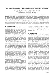
• Problem Dimensions
40 40 45 50
(40,6.447)
(40,6.393)
0.833
0.125
6.5
2
5.375
120 70
2
250
Figure 1: 2D example, problem dimensions

SoilVision Systems Ltd. A Two Dimensional Example Problem Page 6 of 58
• SVFLUX Boundary Conditions
Normal Flux Expression = 0.1 m/yr
• SVFLUX Soil Properties
Zero Flux
Figure 2: 2D example, seepage boundary conditions
0.35
Ksat = 5.0e-06 m/s
Ksat = 1.0e-04 m/s
ky-ratio = 1.0 ky-ratio = 1.0
Volumetric water content = 0.35 Volumetric water content =
A uniform volumetric water content was set by entering a soil water characteristic curve with three points,
(0.0001,0.351), (100,0.35), and (1000,0.349). This soil water characteristic curve was used for both the soils in
the problem.
Steady state seepage solutions do not require that the soil water characteristic curves have an
initial positive slope. An initial positive slope is only required in transient problems where the soil
storage will change with time.

SoilVision Systems Ltd. A Two Dimensional Example Problem Page 7 of 58
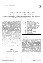
• SVFLUX Flow Regime
7
6
Elevation (m)
5
4
3
2
1
0
0 100 200
Distance Along Flow Direction (m)
Figure 3: 2D example, flow regime
Note that the problem is completely saturated.

SoilVision Systems Ltd. A Two Dimensional Example Problem Page 8 of 58
1.2 CHEMFLUX SOLUTION DATA
• CHEMFLUX Boundary Conditions
Figure 4: 2D example, CHEMFLUX boundary conditions
• CHEMFLUX Soil Properties
Only one soil is used for the problem with these properties:
Longitudinal Dispersivity, α L = 0.5m
Transverse Dispersivity, α T = 0.005m
Diffusion Coefficient, D* = 0.0423m 2 /yr
1.3 SVFLUX GRADIENTS FILE
A gradient file generated by SVFLUX is required for this example. The seepage problem described above has
been included in the database file distributed with the SVFLUX software. To generate the necessary seepage
gradient file, follow these instructions.
1. Open the SVFLUX software.
2. From the menu select Model > Projects/Problems.
3. The Projects/Problems form should now be open. By clicking on plus signs (+)
expand the tree under Examples > 2D > Steady State.
4. Click the problem name ChemFlux2D.
5. Click OK.

SoilVision Systems Ltd. A Two Dimensional Example Problem Page 9 of 58
6. When the problem has opened click the analyze button to run the problem.
When the problem is finished, the necessary gradient file will be created in the solution folder automatically by
SVFLUX. The file is called Examples_ChemFlux2D.GRD (i.e. Project_Problem.GRD). The file is given a
.GRD extension to separate it as a gradient file.
1.4 ADDING A CHEMFLUX PROJECT
The first step in defining a problem is to decide the project under which the problem is going to be organized.
If the project is not yet included you must add the project before proceeding with the problem. In this case, the
problem is placed under a project called Tutorial.
Follow these steps in order to add this project:
1. Select Model > Projects/Problems… from the menu to open the Projects / Problems
form.
2. Click New Project… in the lower left of the form.
3. The Project Properties form is opened along with a prompt asking for a new ProjectID.
4. Type “Tutorial” as the new ProjectID and press OK.
The Project Properties form is where you information specific to each project is stored. This will include the
Project ID, Project Name, Location, Start Date, End Date, Project Notes, client information, contractor and
project engineer information.
The Project ID is the only required information needed to define a project. The rest of the fields
are optional.
The form is opened ready to accept information.

SoilVision Systems Ltd. A Two Dimensional Example Problem Page 10 of 58
It should be noted that once the project is defined it would be identified by the ProjectID throughout the rest of
the program. Also, CHEMFLUX does not allow you to specify two projects with the same ProjectID.
5. Fill out the form with the desired information.
6. To exit this form and return to Projects / Problems click OK. The project information is
automatically saved upon entry.

SoilVision Systems Ltd. A Two Dimensional Example Problem Page 11 of 58
1.5 ADDING A CHEMFLUX PROBLEM
Once a project has been created any number of problems may be stored in it. When the Projects/Problems form
is opened there will be a list of the projects that have been defined. In this case there is only the Tutorial
project. To add a problem:
1. Click on the plus sign and expand the project Tutorial.
2. Select 2D.
3. Click the New Problem button. The New Problem form will open.

SoilVision Systems Ltd. A Two Dimensional Example Problem Page 12 of 58
4. Enter the ProblemID: Example2D. The description is optional.
5. Click the OK button to save the problem and close the New Problem form.
6. The new problem will automatically be opened in the workspace.
You will notice that there is no distinction between steady state and transient state in
CHEMFLUX. This is because all models are considered to be transient state.
1.6 OPENING THE CHEMFLUX PROBLEM
If the problem was just added it will already be open in the workspace. When returning to the problem follow
these steps to open it in the workspace:

SoilVision Systems Ltd. A Two Dimensional Example Problem Page 13 of 58
1. Navigate back to the problem via Tutorial, 2D.
2. Select Example2D.
3. The problem may opened by clicking the OK button or by double clicking on the
ProblemID.
1.7 DEFINING THE CHEMFLUX PROBLEM
The following section provides instructions on how to begin defining the problem in the workspace.
1.7.1 Import SVFLUX Geometry
Geometry must be imported from SVFLUX before any other modeling can be done in CHEMFLUX.
1. Select Model > SVFlux Geometry from the menu.

SoilVision Systems Ltd. A Two Dimensional Example Problem Page 14 of 58
2. Click Browse.
3. Select the SVFlux_Data_J.mdb file that contains the ChemFlux2D problem.
4. Expand the tree and select ChemFlux2D.
5. Press the Import button.
6. Once the import is complete press OK to close the form.
The import includes any regions, region shapes, surfaces, surface grids and elevations. These parts of the
problem definition are fixed in CHEMFLUX. World coordinate system settings and features are also imported
if present, but may be edited in CHEMFLUX.

SoilVision Systems Ltd. A Two Dimensional Example Problem Page 15 of 58
1.7.2 Specify Settings
The next step in defining the problem is to specify the settings that will be used for the problem.
The Settings form will contain information about the current problem System, Units, Time, and contaminant
transport processes.
1. To open the Settings form select Model > Settings in the workspace menu.
2. Check Advection and Dispersion in the Processes section.
3. Enter a Start Time of 0, a Time Increment of 1 yr, and an End Time of 20 yr.
4. Select the Advection tab.

SoilVision Systems Ltd. A Two Dimensional Example Problem Page 16 of 58
5. Choose Import from SVFlux from the Advection Control option.
6. Click Browse.
7. Specify the file Examples_ChemFlux2D_2.grd that was generated by SVFLUX.
8. Press OK to close the Settings form.
It is very important that the .GRD file and the geometry are obtained from the same SVFLUX
problem.

SoilVision Systems Ltd. A Two Dimensional Example Problem Page 17 of 58
1.7.3 Define Material Properties
The next step in defining the problem is to enter the material properties for the single soil that will be used in
the model.
1. Open the Soils form by selecting Model > Soils from the menu or click the soils button,
in the Tools toolbar.
2. Click the New Soil button to create a soil in the database. A unique Soil Index is
generated that is used to reference the soil in other CHEMFLUX forms.
3. Double-click on the new soil to open the Soil Properties form.

SoilVision Systems Ltd. A Two Dimensional Example Problem Page 18 of 58
4. Enter the information above into the appropriate fields on the Description tab
5. Move to the Dispersion tab.
6. Refer to the data provided at the beginning of this tutorial. Enter the Longitudinal
Dispersivity, α L = 0.5m .
7. Enter the Transverse Dispersivity, α T = 0.005m .
8. Select Constant as the Diffusion option.
9. Enter the Diffusion Coefficient, D* = 0.0423m 2 /yr.
10. Close the Soil Properties and Soil Manager forms.
1.7.4 Assign Soils to Regions
A region in CHEMFLUX is the basic building block for a model. A region represents both a physical portion of
soil being modeled and a visualization area in the CHEMFLUX CAD workspace. A region will have a set of
geometric shapes that define its soil boundaries. Also, other modeling objects including features, flux sections,
water tables, text, and line art are defined on any given region.
This problem is divided into three regions, but the same soil will be assigned to each region. To specify the soil
for the regions follow these steps:
1. Open the regions form by clicking the Regions button, at the top of the
workspace.

SoilVision Systems Ltd. A Two Dimensional Example Problem Page 19 of 58
2. Select the Soil Index from the drop-down corresponding to Soil#1 for Region 1.
3. Repeat for Region 2 and Region 3.
4. Click OK to close the form.
1.7.5 Specify Boundary Conditions
The next step is to specify the boundary conditions. Refer to the diagram at the beginning of this tutorial. A
zero flux condition will be defined on sides and base of the problem with various concentration conditions
being applied to the top boundary. The boundary conditions are applied to the outer Region 1; none are applied
to the other 2 regions.
1. Select the “Region 1” region in the drawing space with the mouse.
2. From the menu select Model > Boundaries. The boundary conditions form will open.

SoilVision Systems Ltd. A Two Dimensional Example Problem Page 20 of 58
3. Select the point (0,0) from the list.
4. From the Boundary Condition drop down select a Zero Flux boundary condition.
5. Click the Update button to save the boundary condition to the list.
6. Repeat these steps to define the boundary conditions for the remaining Region 1
segment as shown in the diagram and in the screen-shot above. (Be sure to define a
Zero Flux condition for the last point in the list)
Any boundary condition becomes the boundary condition for the following line segments that
have a Continue boundary condition until a new boundary condition is specified.
1.8 SPECIFY PLOTS
There are many plot types that can be specified to visualize the results of the model. A few will be generated
for this tutorial example problem including a plot of the solution mesh, concentration contours, and water
gradient vectors.
1. Open the Plot Manager form by selecting Model > Plot Manager from the menu.

SoilVision Systems Ltd. A Two Dimensional Example Problem Page 21 of 58
2. The toolbar at the bottom left of the form contains a button for each plot type. Click on
the Contour button to begin adding the first contour plot. The Plot Properties form will
open.
3. Enter the title Concentration.
4. Select c as the variable to plot from the drop-down.
5. Select the PLOT output option.
6. Move to the Time tab and enter a Start Time = 0, a Time Increment = 1, and an End
Time = 20.
7. Move to the Zoom tab and enter X = 100, Y = 0.1, Width = 100, and Height = 6.6.
8. Click OK to close the form and add the plot to the list.
9. Repeat steps 2 – 8 to create the plots shown above. Note that the Mesh plot does not
require entry of a variable.

SoilVision Systems Ltd. A Two Dimensional Example Problem Page 22 of 58
10. Click OK to close the Plot Manager and return to the workspace.
1.9 SPECIFY OUTPUT FILES
There are 4 output file types that can be specified to export the results of the model. One will be generated for
this tutorial example problem: a file to output variables for advanced visualization in the AcuMesh software.
1. Open the Output Manager form by selecting Model > Output Manager from the menu.
2. The toolbar at the bottom left of the form contains a button for each output file type.
Click on the AcuMesh button to begin adding the output file. The Output File
Properties form will open.

SoilVision Systems Ltd. A Two Dimensional Example Problem Page 23 of 58
3. Enter the title AcuMesh.
4. Press the Select All button.
5. Press the Add Selection button.
6. Check the Write File box.
7. Click OK to close the form and add the output file to the list.
8. Click OK to close the Output Manager and return to the workspace.
1.10 ANALYZE
The next step is to analyze the problem. Click the Analyze button located in the left toolbar. This action will
write the descriptor file and open the CHEMFLUX solver. The solver will automatically begin solving the
problem.
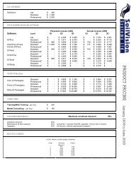
1.11 RESULTS
After the problem has finished solving, the results will be displayed in the form of thumbnail plots within the
CHEMFLUX solver. Right-click the mouse and select Maximize to enlarge any of the thumbnail plots. The
following is a short summary of plots illustrating the movement of the plume through the problem for times of
8 years, 12 years, and 20 years.

SoilVision Systems Ltd. A Two Dimensional Example Problem Page 24 of 58
• Time = 8 years
10.
8.
6.
Concentration
zoom(0,0,250,10)
0.80
0.70
0.60
0.50
0.40
0.30
0.20
0.10
0.00
-0.10
16:36:05 2/20/02
FlexPDE 2.22
Y
4.
2.
0.
0. 50. 100. 150. 200. 250.
X
Examples_2DExample: Cycle=96 Time= 8.0000 dt= 0.1961 p2 Nodes=6375 Cells=3068 RMS Err= 2.9e-4
Integral= 56.74936
The source has been shut off for 3 years

SoilVision Systems Ltd. A Two Dimensional Example Problem Page 25 of 58
• Time = 12 years
10.
8.
Concentration
zoom(0,0,250,10)
0.60
0.50
0.40
0.30
0.20
0.10
0.00
-0.10
16:36:05 2/20/02
FlexPDE 2.22
6.
Y
4.
2.
0.
0. 50. 100. 150. 200. 250.
X
Examples_2DExample: Cycle=129 Time= 12.000 dt= 0.1492 p2 Nodes=7314 Cells=3559 RMS Err= 3.6e-4
Integral= 57.30137

SoilVision Systems Ltd. A Two Dimensional Example Problem Page 26 of 58
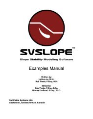
• Time = 20 years
10.
8.
Concentration
zoom(0,0,250,10)
0.30
0.25
0.20
0.15
0.10
0.05
0.00
-0.05
16:36:05 2/20/02
FlexPDE 2.22
6.
Y
4.
2.
0.
0. 50. 100. 150. 200. 250.
X
Examples_2DExample: Cycle=178 Time= 20.000 dt= 0.3099 p2 Nodes=12577 Cells=6140 RMS Err= 3.7e-4
Integral= 61.18735

SoilVision Systems Ltd. A Three Dimensional Example Problem Page 27 of 58
2 A THREE DIMENSIONAL EXAMPLE PROBLEM
The following example will introduce you to the three dimensional model in CHEMFLUX. The model will be
used to investigate if contaminant from a reservoir will travel to a river channel due to advection and dispersion
processes within a 400 day time period. The 400-day time period was chosen as the time necessary to install a
pumping well between the river channel and the reservoir. The well will be used to pump contaminant from
the ground to ensure the plume will not reach the river channel. The example problem begins with a brief
description of the steady state seepage analysis completed to provide CHEMFLUX with computed seepage
gradients. Next a detailed set of instructions guides the user through the creation of the 3D contaminant
transport problem.
ProjectID: Tutorial
ProblemID: Example3D
2.1 STEADY STATE SVFLUX SOLUTION
Advection is known as the process by which solutes are transported by the bulk motion of the flowing
groundwater Freeze & Cherry (1979). The bulk motion of the flowing groundwater or seepage gradients are
solved using SVFLUX. SVFLUX calculates the seepage gradients and writes them to a text file. The
CHEMFLUX solver then reads this text file when calculating the contaminant transport solution. Below is a
description of the seepage problem solved by SVFLUX.
ProjectID: Examples
ProblemID: ChemFlux3D

SoilVision Systems Ltd. A Three Dimensional Example Problem Page 28 of 58
• Problem Dimensions
27
10 1 5 1
2 1
11
24
Figure 5: 3D Example; Problem Dimensions

SoilVision Systems Ltd. A Three Dimensional Example Problem Page 29 of 58
• Surface 1 Grid

SoilVision Systems Ltd. A Three Dimensional Example Problem Page 30 of 58
• Surface 2 Grid

SoilVision Systems Ltd. A Three Dimensional Example Problem Page 31 of 58
• Boundary Conditions
Figure 6: 3D Example; Boundary Conditions
The steady state seepage model is set up to simulate a pond or reservoir a certain distance from
a river channel. The water levels in the reservoir and river channel are set using head boundary
conditions. The level of water in the reservoir is set using a Head Expression = 10.5m set on
surface 2 for the reservoir region. The level of water in the river channel is set using a Head
Expression = 7m set on the line segment extending from point (14,0) to (14,27) on surface 1.
• Soil Properties
There is only one soil in the saturated 3D example problem despite the presence of separate
colors for the two regions. Two regions have been implemented in this problem in order to
apply the necessary boundary conditions. The soil in the problem has a hydraulic conductivity,
ksat = 2.17e –01 m/d.

SoilVision Systems Ltd. A Three Dimensional Example Problem Page 32 of 58
• Flow Regime
Figure 7: 3D Example; Flow Regime
Flow lines show that groundwater is flowing from the reservoir toward the adjacent river
channel. The presence of unsaturated soil near the surface of the problem is causing water to
first flow down to the saturated zone and then move toward the river channel.

SoilVision Systems Ltd. A Three Dimensional Example Problem Page 33 of 58
2.2 CHEMFLUX SOLUTION DATA
• CHEMFLUX Boundary Conditions
Figure 8: 3D example, CHEMFLUX boundary conditions
• CHEMFLUX Soil Properties
Only one soil is used for the problem with these properties:
Longitudinal Dispersivity, α L = 1m
Transverse Dispersivity, α T = 1m
Diffusion Coefficient, D* = 0m 2 /day

SoilVision Systems Ltd. A Three Dimensional Example Problem Page 34 of 58
2.3 SVFLUX GRADIENTS FILE
A gradient file generated by SVFLUX is required for this example. The seepage problem described above has
been included in the database file distributed with the SVFLUX software. To generate the necessary seepage
gradient file, follow these instructions.
1. Open the SVFLUX software.
2. From the menu select Model > Projects/Problems.
3. The Projects/Problems form should now be open. By clicking on plus signs (+)
expand the tree under Examples > 3D > Steady State.
4. Click the problem name ChemFlux3D.
5. Click OK.
6. When the problem has opened click the analyze button to run the problem.
When the problem is finished, the necessary gradient file will be created in the solution folder automatically by
SVFLUX. The file is called Examples_ChemFlux3D.GRD (i.e. Project_Problem.GRD). The file is given a
.GRD extension to separate it as a gradient file.
2.4 ADDING A CHEMFLUX PROJECT
The first step in defining a problem is to decide the project under which the problem is going to be organized.
If the project is not yet included you must add the project before proceeding with the problem. In this case, the
problem is placed under a project called Tutorial.
Follow these steps in order to add this project:
1. Select Model > Projects/Problems… from the menu to open the Projects / Problems
form.
2. Click New Project… in the lower left of the form.
3. The Project Properties form is opened along with a prompt asking for a new ProjectID.
4. Type “Tutorial” as the new ProjectID and press OK.
The Project Properties form is where you information specific to each project is stored. This will include the
Project ID, Project Name, Location, Start Date, End Date, Project Notes, client information, contractor and
project engineer information.
The Project ID is the only required information needed to define a project. The rest of the fields
are optional.

SoilVision Systems Ltd. A Three Dimensional Example Problem Page 35 of 58
The form is opened ready to accept information.
Note that once the project is defined it will be identified by the ProjectID throughout the rest of the program.
Also, CHEMFLUX does not allow you to specify two projects with the same ProjectID.
5. Fill out the form with the desired information.
6. To exit this form and return to Projects / Problems click OK. The project information is
automatically saved upon entry.

SoilVision Systems Ltd. A Three Dimensional Example Problem Page 36 of 58
2.5 ADDING A CHEMFLUX PROBLEM
Once a project has been created any number of problems may be stored in it. When the Projects/Problems form
is opened there will be a list of the projects that have been defined. In this case there is only the Tutorial
project. To add a problem:
1. Click on the plus sign and expand the project Tutorial.
2. Select 3D.
3. Click the New Problem button. The New Problem form will open.

SoilVision Systems Ltd. A Three Dimensional Example Problem Page 37 of 58
4. Enter the ProblemID: Example3D. The description is optional.
5. Click the OK button to save the problem and close the New Problem form.
6. The new problem will automatically be opened in the workspace.
2.6 OPENING THE PROBLEM
If the problem was just added it will already be open in the workspace. When returning to the problem follow
these steps to open it in the workspace:

SoilVision Systems Ltd. A Three Dimensional Example Problem Page 38 of 58
1. Navigate back to the problem via Tutorial, 3D.
2. Select Example3D.
3. The problem may opened by clicking the OK button or by double clicking on the
ProblemID.
2.7 DEFINING THE PROBLEM
The following section provides instructions on how to begin defining the problem in the workspace.
2.7.1 Import SVFLUX Geometry
Geometry must be imported from SVFLUX before any other modeling can be done in CHEMFLUX.
1. Select Model > SVFlux Geometry from the menu.

SoilVision Systems Ltd. A Three Dimensional Example Problem Page 39 of 58
2. Click Browse.
3. Select the SVFlux_Data_J.mdb file that contains the ChemFlux3D problem.
4. Expand the tree and select ChemFlux3D.
5. Press the Import button.
6. Once the import is complete press OK to close the form.
The import includes any regions, region shapes, surfaces, surface grids and elevations. These parts of the
problem definition are fixed in CHEMFLUX. World coordinate system settings and features are also imported
if present, but may be edited in CHEMFLUX.
2.7.2 Specify Settings
The next step in defining the problem is to specify the settings that will be used for the problem.

SoilVision Systems Ltd. A Three Dimensional Example Problem Page 40 of 58
The Settings form will contain information about the current problem System, Units, Time, and contaminant
transport processes.
1. To open the Settings form select Model > Settings in the workspace menu.
2. Check Advection and Dispersion in the Processes section.
3. Enter a Start Time of 0, a Time Increment of 50 days, and an End Time of 400 days.
4. Select the Advection tab.

SoilVision Systems Ltd. A Three Dimensional Example Problem Page 41 of 58
5. Choose Import from SVFlux from the Advection Control option.
6. Click Browse.
7. Specify the file Examples_ChemFlux3D_2.grd that was generated by SVFLUX.
It is very important that the .GRD file and the geometry are obtained from the same SVFLUX
problem.
In order to improve solution time for the purposes of this tutorial certain finite-element options will be set. The
finite element mesh node limit and grid spacing will be set to generate a simpler mesh that will increase the
solution time.
8. Press the FEM Options button to open the FEM Options form.
9. Set the NODELIMIT as 800. (This is the student version maximum)
10. Set the NGRID parameter to 5. (This is the student version maximum)
11. Press OK to close the FEM Options form.
12. Press OK to close the Settings form.

SoilVision Systems Ltd. A Three Dimensional Example Problem Page 42 of 58
2.7.3 Define Material Properties
The next step in defining the problem is to enter the material properties for the single soil that will be used in
the model.
1. Open the Soils form by selecting Model > Soils from the menu or click the soils button,
in the Tools toolbar.
2. Click the New Soil button to create a soil in the database. A unique Soil Index is
generated that is used to reference the soil in other CHEMFLUX forms.
3. Double-click on the new soil to open the Soil Properties form.

SoilVision Systems Ltd. A Three Dimensional Example Problem Page 43 of 58
4. Enter the information above into the appropriate fields on the Description tab
5. Move to the Dispersion tab.

SoilVision Systems Ltd. A Three Dimensional Example Problem Page 44 of 58
6. Refer to the data provided at the beginning of this tutorial. Enter the Longitudinal
Dispersivity, α L = 1m .
7. Enter the Transverse Dispersivity, α T = 1m .
8. The Diffusion option is set to Constant as the gradient file specified does not contain
volumetric water content, which is required to define a diffusion curve.
9. Enter the Diffusion Coefficient, D* = 0m 2 /day.
10. Close the Soil Properties and Soil Manager forms.
2.7.4 Specifying a Soil by Region and Layer
Each region will cut through all the layers in a problem creating a separate “block” on each layer. Each block
can be assigned a soil or be left as void. A void area is essentially air space. In this problem all “blocks” will be
assigned a soil.
1. Select “Slope” in the Region Selector.
2. Press the Region Soils button, at the top of the workspace to open the Region Soils
form.

SoilVision Systems Ltd. A Three Dimensional Example Problem Page 45 of 58
3. Select the soil from the drop-down for Layer 1.
4. Close the form using the OK button.
5. Select “Reservoir” in the Region Selector.
6. Press the Region Soils button, at the top of the workspace to open the Region Soils
form.
7. Select the soil from the drop-down for Layer 1.
8. Close the form using the OK button.
2.7.5 Specify Boundary Conditions
The next step is to specify the boundary conditions on the region shapes. The only boundary condition that is
required for this problem is to set a Concentration Expression condition for the reservoir region on Surface 2.
The steps for specifying the boundary condition are thus:
1. Select the “Reservoir” region in the drawing space.
2. From the menu select Model > Boundaries. The boundary conditions form will open
and display the boundary conditions for Surface 1.
3. Select Surface 2 from the Surface option box.

SoilVision Systems Ltd. A Three Dimensional Example Problem Page 46 of 58
4. Select Concentration Expression from the Boundary Condition combo box under the
Surface Boundary Condition section. This will cause the Concentration Expression
box to be enabled.
5. In the Expression box enter a concentration of 1.
6. Click the OK button to close the form.
2.8 SPECIFY PLOTS
There are many plot types that can be specified to visualize the results of the model. A few will be generated
for this tutorial example problem including a plot of the concentration contours, solution mesh, and water
gradient vectors.
1. Open the Plot Manager form by selecting Model > Plot Manager from the menu.

SoilVision Systems Ltd. A Three Dimensional Example Problem Page 47 of 58
2. The toolbar at the bottom left of the form contains a button for each plot type. Click on
the Contour button to begin adding the first contour plot. The Plot Properties form will
open.
3. Enter the title Concentration.
4. Select c as the variable to plot from the drop-down.
5. Select the PLOT output option.
6. Move to the Time tab.
7. Press the Arrow to put the problem times in the plot time fields.
8. Move to the Projection tab.
9. Select Plane Projection option.
10. Select Y from the Coordinate Direction drop-down.

SoilVision Systems Ltd. A Three Dimensional Example Problem Page 48 of 58
11. Enter 14 in the Coordinate field. This will generate a 2D slice at Y = 14m on which the
concentration contours will be plotted.
12. Click OK to close the form and add the plot to the list.
13. Repeat these steps 2 – 12 to create the plots shown above. Note that the Mesh plot
does not require entry of a variable.
14. Click OK to close the Plot Manager and return to the workspace.
2.9 SPECIFY OUTPUT FILES
There are 4 output file types that can be specified to export the results of the model. One will be generated for
this tutorial example problem: a file to output the results to AcuMesh for advanced visualization.
1. Open the Output Manager form by selecting Model > Output Manager from the menu.
2. The toolbar at the bottom left of the form contains a button for each output file type.
Click on the AcuMesh button to begin adding the output file. The Output File
Properties form will open.

SoilVision Systems Ltd. A Three Dimensional Example Problem Page 49 of 58
3. Enter the title TutorialAcuMesh.
4. Select variables c, vx, vy, and vz in the list.
5. Press the Add Selection button.
6. Check the Write File box.
7. Click OK to close the form and add the output file to the list.
8. Click OK to close the Output Manager and return to the workspace.
2.10 ANALYZE
The next step is to analyze the problem. Click the Analyze button located in the left toolbar. This action will
write the descriptor file and open the CHEMFLUX solver. The solver will automatically begin solving the
problem.
2.11 RESULTS
After the problem has finished solving, the results will be displayed in the form of thumbnail plots within the
CHEMFLUX solver. Right-click the mouse and select Maximize to enlarge any of the thumbnail plots. This
section will give a brief analysis for each plot that was generated.

SoilVision Systems Ltd. A Three Dimensional Example Problem Page 50 of 58
2.11.1 Solution Mesh
The Mesh plot displays the finite-element mesh generated by the solver. The mesh is automatically refined in
critical areas. Right-click on the plot and select Rotate to enable the rotate window.

SoilVision Systems Ltd. A Three Dimensional Example Problem Page 51 of 58
2.11.2 Concentration Contours
In this contour plot it can be seen the concentration is equal to 1 at the reservoir and decreases to 0 at the river.

SoilVision Systems Ltd. A Three Dimensional Example Problem Page 52 of 58
2.11.3 Flow Vectors
Gradient Vectors show both the direction and the magnitude of the flow at specific points in the problem.
Vectors illustrate that flow is from right to left towards the river in this view with higher gradients near the
reservoir.
2.11.4 AcuMesh
The following is a short summary of plots created in AcuMesh illustrating the movement of the plume through
the problem for times of 50 days, 100 days, and 400 days. Note that the plume does not reach the river channel
in within the 400 day time period.

SoilVision Systems Ltd. A Three Dimensional Example Problem Page 53 of 58
• Time = 50 days

SoilVision Systems Ltd. A Three Dimensional Example Problem Page 54 of 58
• Time = 100 days

SoilVision Systems Ltd. A Three Dimensional Example Problem Page 55 of 58
• Time = 400 days

SoilVision Systems Ltd. References Page 56 of 58
3 REFERENCES
C.W. Fetter, 1994. Applied Hydrogeology, Third Edition. Prentice-Hall, Inc. Upper Saddle River,
New Jersey.
C.W. Fetter, 1993. Contaminant Hydrogeology. MacMillan Publishing Company. New York, New
York.
D. G. Fredlund and H. Rahardjo, 1993. Soil Mechanics for Unsaturated Soils. John Wiley & Sons,
New York
FlexPDE 3.x Reference Manual, 1999. PDE Solutions Inc. Antioch, CA 94509
Jacob Bear, 1972. Dynamics of Fluids in Porous Media. Dover Publications Inc., New York
Jacob Bear, 1979. Hydraulics of Groundwater. McGraw-Hill, New York.
Jason S. Pentland, 2000. Use of a General Partial Differential Equation Solver for Solution of Heat
and Mass Transfer Problems in Soils. University of Saskatchewan, Canada
Nguyen Thi Minh Thieu, 1999. Solution of Saturated/Unsaturated Seepage Problems Using a
General Partial Differential Equation Solver. University of Saskatchewan, Canada
R. Allan Freeze and John A. Cherry, 1979. Groundwater. Prentice –Hall, Inc., Englewood Cliffs,
New Jersey
Tecplot User’s Manual, version 8.0, 1999. Amtec Engineering Inc. Bellevue, WA 98009-3633

SoilVision Systems Ltd. Index Page 57 of 58
4 INDEX
Advection, 15, 16, 27, 40, 41
Boundaries, 19, 45
Boundary Conditions, 6, 8, 19, 31, 33, 45
Concentration, 21, 45, 46, 47, 51
Contaminant, 56
Diffusion, 8, 18, 33, 44
Dispersion, 15, 18, 40, 43
Dispersivity, 8, 18, 33, 44
Fill, 10, 35
Geometry, 13, 38
Gradient, 52
Grid, 29, 30
Head Expression, 31
Mass, 56
Mesh, 21, 48, 50
Output, 22, 23, 48, 49
Output Files, 22, 48
Plots, 20, 46
Problem, 5, 9, 11, 12, 13, 27, 28, 34, 36, 37,
38
ProblemID, 5, 12, 13, 27, 37, 38
Problems, 8, 9, 10, 11, 34, 35, 36, 56
Processes, 15, 40
Project, 9, 34
ProjectID, 5, 9, 10, 27, 34, 35
Projects, 8, 9, 10, 11, 34, 35, 36
Properties, 6, 8, 9, 17, 18, 21, 22, 31, 33, 34,
42, 44, 47, 48
Region, 19, 20, 44, 45
Regions, 18
Seepage, 56
Selector, 44, 45
Soil, 6, 8, 17, 18, 19, 31, 33, 42, 44, 56
Soils, 17, 18, 42, 44, 45, 56
Solution, 5, 8, 27, 33, 50, 56
Steady-State, 5
Surface, 29, 30, 45, 46
SVFLUX, 2, 5, 6, 7, 8, 9, 13, 16, 27, 34, 38,
41
Tecplot, 48, 52, 56
Time, 15, 21, 24, 25, 26, 40, 47, 53, 54, 55
Zero Flux, 20
Zoom, 21

SoilVision Systems Ltd. Index Page 58 of 58
This page is intentionally left blank.