Elementary Number Theory - Index of
Elementary Number Theory - Index of
Elementary Number Theory - Index of

Create successful ePaper yourself
Turn your PDF publications into a flip-book with our unique Google optimized e-Paper software.
This is page i<br />
Printer: Opaque this<br />
<strong>Elementary</strong> <strong>Number</strong> <strong>Theory</strong><br />
William Stein<br />
October 2005
ii<br />
To my students and my wife, Clarita Lefthand.
Contents<br />
This is page iii<br />
Printer: Opaque this<br />
Preface 3<br />
1 Prime <strong>Number</strong>s 5<br />
1.1 Prime Factorization . . . . . . . . . . . . . . . . . . . . . . 5<br />
1.2 The Sequence <strong>of</strong> Prime <strong>Number</strong>s . . . . . . . . . . . . . . . 13<br />
1.3 Exercises . . . . . . . . . . . . . . . . . . . . . . . . . . . . 20<br />
2 The Ring <strong>of</strong> Integers Modulo n 21<br />
2.1 Congruences Modulo n . . . . . . . . . . . . . . . . . . . . . 21<br />
2.2 The Chinese Remainder Theorem . . . . . . . . . . . . . . . 27<br />
2.3 Quickly Computing Inverses and Huge Powers . . . . . . . . 29<br />
2.4 Finding Primes . . . . . . . . . . . . . . . . . . . . . . . . . 33<br />
2.5 The Structure <strong>of</strong> (Z/pZ) ∗ . . . . . . . . . . . . . . . . . . . 34<br />
2.6 Exercises . . . . . . . . . . . . . . . . . . . . . . . . . . . . 38<br />
3 Public-Key Cryptography 43<br />
3.1 The Diffie-Hellman Key Exchange . . . . . . . . . . . . . . 46<br />
3.2 The RSA Cryptosystem . . . . . . . . . . . . . . . . . . . . 51<br />
3.3 Attacking RSA . . . . . . . . . . . . . . . . . . . . . . . . . 54<br />
3.4 Exercises . . . . . . . . . . . . . . . . . . . . . . . . . . . . 58<br />
4 Quadratic Reciprocity 59<br />
4.1 Statement <strong>of</strong> the Quadratic Reciprocity Law . . . . . . . . 60<br />
4.2 Euler’s Criterion . . . . . . . . . . . . . . . . . . . . . . . . 62
Contents 1<br />
4.3 First Pro<strong>of</strong> <strong>of</strong> Quadratic Reciprocity . . . . . . . . . . . . . 63<br />
4.4 A Pro<strong>of</strong> <strong>of</strong> Quadratic Reciprocity Using Gauss Sums . . . . 68<br />
4.5 Finding Square Roots . . . . . . . . . . . . . . . . . . . . . 72<br />
4.6 Exercises . . . . . . . . . . . . . . . . . . . . . . . . . . . . 74<br />
5 Continued Fractions 77<br />
5.1 Finite Continued Fractions . . . . . . . . . . . . . . . . . . 78<br />
5.2 Infinite Continued Fractions . . . . . . . . . . . . . . . . . . 83<br />
5.3 The Continued Fraction <strong>of</strong> e . . . . . . . . . . . . . . . . . . 88<br />
5.4 Quadratic Irrationals . . . . . . . . . . . . . . . . . . . . . . 91<br />
5.5 Recognizing Rational <strong>Number</strong>s . . . . . . . . . . . . . . . . 96<br />
5.6 Sums <strong>of</strong> Two Squares . . . . . . . . . . . . . . . . . . . . . 97<br />
5.7 Exercises . . . . . . . . . . . . . . . . . . . . . . . . . . . . 100<br />
6 Elliptic Curves 103<br />
6.1 The Definition . . . . . . . . . . . . . . . . . . . . . . . . . 103<br />
6.2 The Group Structure on an Elliptic Curve . . . . . . . . . . 104<br />
6.3 Integer Factorization Using Elliptic Curves . . . . . . . . . 107<br />
6.4 Elliptic Curve Cryptography . . . . . . . . . . . . . . . . . 113<br />
6.5 Elliptic Curves Over the Rational <strong>Number</strong>s . . . . . . . . . 117<br />
6.6 Exercises . . . . . . . . . . . . . . . . . . . . . . . . . . . . 122<br />
7 Computational <strong>Number</strong> <strong>Theory</strong> 125<br />
7.1 Prime <strong>Number</strong>s . . . . . . . . . . . . . . . . . . . . . . . . . 127<br />
7.2 The Ring <strong>of</strong> Integers Modulo n . . . . . . . . . . . . . . . . 133<br />
7.3 Public-Key Cryptography . . . . . . . . . . . . . . . . . . . 141<br />
7.4 Quadratic Reciprocity . . . . . . . . . . . . . . . . . . . . . 147<br />
7.5 Continued Fractions . . . . . . . . . . . . . . . . . . . . . . 150<br />
7.6 Elliptic Curves . . . . . . . . . . . . . . . . . . . . . . . . . 154<br />
7.7 Exercises . . . . . . . . . . . . . . . . . . . . . . . . . . . . 162<br />
Answers and Hints 165<br />
References 173
2 Contents
Preface<br />
This is page 3<br />
Printer: Opaque this<br />
This is a textbook about prime numbers, congruences, basic public-key<br />
cryptography, quadratic reciprocity, continued fractions, elliptic curves, and<br />
number theory algorithms. We assume the reader has some familiarity with<br />
groups, rings, and fields, and for Chapter 7 some programming experience.<br />
This book grew out <strong>of</strong> an undergraduate course that the author taught at<br />
Harvard University in 2001 and 2002.<br />
Notation and Conventions. We let N = {1, 2, 3, . . .} denote the natural<br />
numbers, and use the standard notation Z, Q, R, and C for the rings <strong>of</strong><br />
integer, rational, real, and complex numbers, respectively. In this book we<br />
will use the words proposition, theorem, lemma, and corollary as follows.<br />
Usually a proposition is a less important or less fundamental assertion, a<br />
theorem a deeper culmination <strong>of</strong> ideas, a lemma something that we will<br />
use later in this book to prove a proposition or theorem, and a corollary<br />
an easy consequence <strong>of</strong> a proposition, theorem, or lemma.<br />
Acknowledgements. Brian Conrad and Ken Ribet made a large number<br />
<strong>of</strong> clarifying comments and suggestions throughout the book. Baurzhan<br />
Bektemirov, Lawrence Cabusora, and Keith Conrad read drafts <strong>of</strong> this book<br />
and made many comments. Frank Calegari used the course when teaching<br />
Math 124 at Harvard, and he and his students provided much feedback.<br />
Noam Elkies made comments and suggested Exercise 4.5. Seth Kleinerman<br />
wrote a version <strong>of</strong> Section 5.3 as a class project. Samit Dasgupta, George<br />
Stephanides, Kevin Stern, and Heidi Williams all suggested corrections. I
4 Contents<br />
also benefited from conversations with Henry Cohn and David Savitt. I<br />
used Emacs, L A TEX, and Python in the preparation <strong>of</strong> this book.
1<br />
Prime <strong>Number</strong>s<br />
This is page 5<br />
Printer: Opaque this<br />
In Section 1.1 we describe how the integers are built out <strong>of</strong> the prime<br />
numbers 2, 3, 5, 7, 11, . . .. In Section 1.2 we discuss theorems about the set<br />
<strong>of</strong> primes numbers, starting with Euclid’s pro<strong>of</strong> that this set is infinite,<br />
then explore the distribution <strong>of</strong> primes via the prime number theorem and<br />
the Riemann Hypothesis (without pro<strong>of</strong>s).<br />
1.1 Prime Factorization<br />
1.1.1 Primes<br />
The set <strong>of</strong> natural numbers is<br />
and the set <strong>of</strong> integers is<br />
N = {1, 2, 3, 4, . . .},<br />
Z = {. . . , −2, −1, 0, 1, 2, . . .}.<br />
Definition 1.1.1 (Divides). If a, b ∈ Z we say that a divides b, written<br />
a | b, if ac = b for some c ∈ Z. In this case we say a is a divisor <strong>of</strong> b. We say<br />
that a does not divide b, written a ∤ b, if there is no c ∈ Z such that ac = b.<br />
For example, we have 2 | 6 and −3 | 15. Also, all integers divide 0, and 0<br />
divides only 0. However, 3 does not divide 7 in Z.<br />
Remark 1.1.2. The notation b . : a for “b is divisible by a” is common in<br />
Russian literature on number theory.
6 1. Prime <strong>Number</strong>s<br />
Definition 1.1.3 (Prime and Composite). An integer n > 1 is prime<br />
if it the only positive divisors <strong>of</strong> n are 1 and n. We call n composite if n is<br />
not prime.<br />
The number 1 is neither prime nor composite. The first few primes <strong>of</strong> N<br />
are<br />
2, 3, 5, 7, 11, 13, 17, 19, 23, 29, 31, 37, 41, 43, 47, 53, 59, 61, 67, 71, 73, 79, . . . ,<br />
and the first few composites are<br />
4, 6, 8, 9, 10, 12, 14, 15, 16, 18, 20, 21, 22, 24, 25, 26, 27, 28, 30, 32, 33, 34, . . . .<br />
Remark 1.1.4. J. H. Conway argues in [Con97, viii] that −1 should be<br />
considered a prime, and in the 1914 table [Leh14], Lehmer considers 1 to<br />
be a prime. In this book we consider neither −1 nor 1 to be prime.<br />
Every natural number is built, in a unique way, out <strong>of</strong> prime numbers:<br />
Theorem 1.1.5 (Fundamental Theorem <strong>of</strong> Arithmetic). Every natural<br />
number can be written as a product <strong>of</strong> primes uniquely up to order.<br />
Note that primes are the products with only one factor and 1 is the<br />
empty product.<br />
Remark 1.1.6. Theorem 1.1.5, which we will prove in Section 1.1.4, is trickier<br />
to prove than you might first think. For example, unique factorization<br />
fails in the ring<br />
Z[ √ −5] = {a + b √ −5 : a, b ∈ Z} ⊂ C,<br />
where 6 factors into irreducible elements in two different ways:<br />
2 · 3 = 6 = (1 + √ −5) · (1 − √ −5).<br />
1.1.2 The Greatest Common Divisor<br />
We will use the notion <strong>of</strong> greatest common divisor <strong>of</strong> two integers to prove<br />
that if p is a prime and p | ab, then p | a or p | b. Proving this is the key<br />
step in our pro<strong>of</strong> <strong>of</strong> Theorem 1.1.5.<br />
Definition 1.1.7 (Greatest Common Divisor). Let<br />
gcd(a, b) = max {d ∈ Z : d | a and d | b} ,<br />
unless both a and b are 0 in which case gcd(0, 0) = 0.<br />
For example, gcd(1, 2) = 1, gcd(6, 27) = 3, and for any a, gcd(0, a) =<br />
gcd(a, 0) = a.<br />
If a ≠ 0, the greatest common divisor exists because if d | a then d ≤ a,<br />
and there are only a positive integers ≤ a. Similarly, the gcd exists when<br />
b ≠ 0.
Lemma 1.1.8. For any integers a and b we have<br />
1.1 Prime Factorization 7<br />
gcd(a, b) = gcd(b, a) = gcd(±a, ±b) = gcd(a, b − a) = gcd(a, b + a).<br />
Pro<strong>of</strong>. We only prove that gcd(a, b) = gcd(a, b − a), since the other cases<br />
are proved in a similar way. Suppose d | a and d | b, so there exist integers<br />
c 1 and c 2 such that dc 1 = a and dc 2 = b. Then b−a = dc 2 −dc 1 = d(c 2 −c 1 ),<br />
so d | b − a. Thus gcd(a, b) ≤ gcd(a, b − a), since the set over which we are<br />
taking the max for gcd(a, b) is a subset <strong>of</strong> the set for gcd(a, b − a). The<br />
same argument with a replaced by −a and b replaced by b − a, shows that<br />
gcd(a, b − a) = gcd(−a, b − a) ≤ gcd(−a, b) = gcd(a, b), which proves that<br />
gcd(a, b) = gcd(a, b − a).<br />
Lemma 1.1.9. Suppose a, b, n ∈ Z. Then gcd(a, b) = gcd(a, b − an).<br />
Pro<strong>of</strong>. By repeated application <strong>of</strong> Lemma 1.1.8, we have<br />
gcd(a, b) = gcd(a, b − a) = gcd(a, b − 2a) = · · · = gcd(a, b − 2n).<br />
Assume for the moment that we have already proved Theorem 1.1.5.<br />
A natural (and naive!) way to compute gcd(a, b) is to factor a and b as<br />
a product <strong>of</strong> primes using Theorem 1.1.5; then the prime factorization <strong>of</strong><br />
gcd(a, b) can read <strong>of</strong>f from that <strong>of</strong> a and b. For example, if a = 2261 and<br />
b = 1275, then a = 7 · 17 · 19 and b = 3 · 5 2 · 17, so gcd(a, b) = 17. It turns<br />
out that the greatest common divisor <strong>of</strong> two integers, even huge numbers<br />
(millions <strong>of</strong> digits), is surprisingly easy to compute using Algorithm 1.1.12<br />
below, which computes gcd(a, b) without factoring a or b.<br />
To motivate Algorithm 1.1.12, we compute gcd(2261, 1275) in a different<br />
way. First, we recall a helpful fact.<br />
Proposition 1.1.10. Suppose that a and b are integers with b ≠ 0. Then<br />
there exists unique integers q and r such that 0 ≤ r < |b| and a = bq + r.<br />
Pro<strong>of</strong>. For simplicity, assume that both a and b are positive (we leave the<br />
general case to the reader). Let Q be the set <strong>of</strong> all nonnegative integers n<br />
such that a − bn is nonnegative. Then Q is nonempty because 0 ∈ Q and Q<br />
is bounded because a − bn < 0 for all n > a/b. Let q be the largest element<br />
<strong>of</strong> Q. Then r = a − bq < b, otherwise q + 1 would also be in Q. Thus q<br />
and r satisfy the existence conclusion.<br />
To prove uniqueness, suppose for the sake <strong>of</strong> contradiction that q ′ and<br />
r ′ = a − bq ′ also satisfy the conclusion but that q ′ ≠ q. Then q ′ ∈ Q since<br />
r ′ = a − bq ′ ≥ 0, so q ′ < q and we can write q ′ = q − m for some m > 0.<br />
But then r ′ = a − bq ′ = a − b(q − m) = a − bq + bm = r + bm > b since<br />
r ≥ 0, a contradiction.
8 1. Prime <strong>Number</strong>s<br />
For us an algorithm is a finite sequence <strong>of</strong> instructions that can be followed<br />
to perform a specific task, such as a sequence <strong>of</strong> instructions in a<br />
computer program, which must terminate on any valid input. The word “algorithm”<br />
is sometimes used more loosely (and sometimes more precisely)<br />
than defined here, but this definition will suffice for us.<br />
Algorithm 1.1.11 (Division Algorithm). Suppose a and b are integers<br />
with b ≠ 0. This algorithm computes integers q and r such that 0 ≤ r < |b|<br />
and a = bq + r. We will not describe the actual steps <strong>of</strong> this algorithm, since<br />
it is just the familiar long division algorithm.<br />
We use the division algorithm repeatedly to compute gcd(2261, 1275).<br />
Dividing 2261 by 1275 we find that<br />
2261 = 1 · 1275 + 986,<br />
so q = 1 and r = 986. Notice that if a natural number d divides both 2261<br />
and 1275, then d divides their difference 986 and d still divides 1275. On<br />
the other hand, if d divides both 1275 and 986, then it has to divide their<br />
sum 2261 as well! We have made progress:<br />
gcd(2261, 1275) = gcd(1275, 986).<br />
This equality also follows by repeated application <strong>of</strong> Lemma 1.1.8. Repeating,<br />
we have<br />
1275 = 1 · 986 + 289,<br />
so gcd(1275, 986) = gcd(986, 289). Keep going:<br />
986 = 3 · 289 + 119<br />
289 = 2 · 119 + 51<br />
119 = 2 · 51 + 17.<br />
Thus gcd(2261, 1275) = · · · = gcd(51, 17), which is 17 because 17 | 51. Thus<br />
gcd(2261, 1275) = 17.<br />
Aside from some tedious arithmetic, that computation was systematic, and<br />
it was not necessary to factor any integers (which is something we do not<br />
know how to do quickly if the numbers involved have hundreds <strong>of</strong> digits).<br />
Algorithm 1.1.12 (Greatest Common Division). Given integers a, b,<br />
this algorithm computes gcd(a, b).<br />
1. [Assume a > b ≥ 0] We have gcd(a, b) = gcd(|a|, |b|) = gcd(|b|, |a|),<br />
so we may replace a and b by their absolute value and hence assume<br />
a, b ≥ 0. If a = b output a and terminate. Swapping if necessary we<br />
assume a > b.
1.1 Prime Factorization 9<br />
2. [Quotient and Remainder] Using Algorithm 1.1.11, write a = bq+r, with<br />
0 ≤ r < b and q ∈ Z.<br />
3. [Finished?] If r = 0 then b | a, so we output b and terminate.<br />
4. [Shift and Repeat] Set a ← b and b ← r, then go to step 2.<br />
Pro<strong>of</strong>. Lemmas 1.1.8–1.1.9 imply that gcd(a, b) = gcd(b, r) so the gcd does<br />
not change in step 4. Since the remainders form a decreasing sequence <strong>of</strong><br />
nonnegative integers, the algorithm terminates.<br />
See Section 7.1.1 for an implementation <strong>of</strong> Algorithm 1.1.12.<br />
Example 1.1.13. Set a = 15 and b = 6.<br />
15 = 6 · 2 + 3 gcd(15, 6) = gcd(6, 3)<br />
6 = 3 · 2 + 0 gcd(6, 3) = gcd(3, 0) = 3<br />
Note that we can just as easily do an example that is ten times as big, an<br />
observation that will be important in the pro<strong>of</strong> <strong>of</strong> Theorem 1.1.17 below.<br />
Example 1.1.14. Set a = 150 and b = 60.<br />
150 = 60 · 2 + 30 gcd(150, 60) = gcd(60, 30)<br />
60 = 30 · 2 + 0 gcd(60, 30) = gcd(30, 0) = 30<br />
Lemma 1.1.15. For any integers a, b, n, we have<br />
gcd(an, bn) = gcd(a, b) · n.<br />
Pro<strong>of</strong>. The idea is to follow Example 1.1.14; we step through Euclid’s algorithm<br />
for gcd(an, bn) and note that at every step the equation is the<br />
equation from Euclid’s algorithm for gcd(a, b) but multiplied through by n.<br />
For simplicity, assume that both a and b are positive. We will prove the<br />
lemma by induction on a + b. The statement is true in the base case when<br />
a + b = 2, since then a = b = 1. Now assume a, b are arbitrary with a ≤ b.<br />
Let q and r be such that a = bq + r and 0 ≤ r < b. Then by Lemmas 1.1.8–<br />
1.1.9, we have gcd(a, b) = gcd(b, r). Multiplying a = bq + r by n we see<br />
that an = bnq + rn, so gcd(an, bn) = gcd(bn, rn). Then<br />
b + r = b + (a − bq) = a − b(q − 1) ≤ a < a + b,<br />
so by induction gcd(bn, rn) = gcd(b, r) · n. Since gcd(a, b) = gcd(b, r), this<br />
proves the lemma.<br />
Lemma 1.1.16. Suppose a, b, n ∈ Z are such that n | a and n | b. Then<br />
n | gcd(a, b).<br />
Pro<strong>of</strong>. Since n | a and n | b, there are integers c 1 and c 2 , such that a = nc 1<br />
and b = nc 2 . By Lemma 1.1.15, gcd(a, b) = gcd(nc 1 , nc 2 ) = n gcd(c 1 , c 2 ),<br />
so n divides gcd(a, b).
10 1. Prime <strong>Number</strong>s<br />
At this point it would be natural to formally analyze the complexity <strong>of</strong><br />
Algorithm 1.1.12. We will not do this, because the main reason we introduced<br />
Algorithm 1.1.12 is that it will allow us to prove Theorem 1.1.5,<br />
and we have not chosen to formally analyze the complexity <strong>of</strong> the other<br />
algorithms in this book. For an extensive analysis <strong>of</strong> the complexity <strong>of</strong><br />
Algorithm 1.1.12, see [Knu98, §4.5.3].<br />
With Algorithm 1.1.12, we can prove that if a prime divides the product<br />
<strong>of</strong> two numbers, then it has got to divide one <strong>of</strong> them. This result is the<br />
key to proving that prime factorization is unique.<br />
Theorem 1.1.17 (Euclid). Let p be a prime and a, b ∈ N. If p | ab then<br />
p | a or p | b.<br />
You might think this theorem is “intuitively obvious”, but that might be<br />
because the fundamental theorem <strong>of</strong> arithmetic (Theorem 1.1.5) is deeply<br />
ingrained in your intuition. Yet Theorem 1.1.17 will be needed in our pro<strong>of</strong><br />
<strong>of</strong> the fundamental theorem <strong>of</strong> arithmetic.<br />
Pro<strong>of</strong> <strong>of</strong> Theorem 1.1.17. If p | a we are done. If p ∤ a then gcd(p, a) = 1,<br />
since only 1 and p divide p. By Lemma 1.1.15, gcd(pb, ab) = b. Since p | pb<br />
and, by hypothesis, p | ab, it follows from Lemma 1.1.15 that<br />
p | gcd(pb, ab) = b.<br />
1.1.3 <strong>Number</strong>s Factor as Products <strong>of</strong> Primes<br />
In this section, we prove that every natural number factors as a product<br />
<strong>of</strong> primes. Then we discuss the difficulty <strong>of</strong> finding such a decomposition<br />
in practice. We will wait until Section 1.1.4 to prove that factorization is<br />
unique.<br />
As a first example, let n = 1275. The sum <strong>of</strong> the digits <strong>of</strong> n is divisible<br />
by 3, so n is divisible by 3 (see Proposition 2.1.3), and we have n = 3 · 425.<br />
The number 425 is divisible by 5, since its last digit is 5, and we have<br />
1275 = 3 · 5 · 85. Again, dividing 85 by 5, we have 1275 = 3 · 5 2 · 17,<br />
which is the prime factorization <strong>of</strong> 1275. Generalizing this process proves<br />
the following proposition:<br />
Proposition 1.1.18. Every natural number is a product <strong>of</strong> primes.<br />
Pro<strong>of</strong>. Let n be a natural number. If n = 1, then n is the empty product<br />
<strong>of</strong> primes. If n is prime, we are done. If n is composite, then n = ab with<br />
a, b < n. By induction, a and b are products <strong>of</strong> primes, so n is also a product<br />
<strong>of</strong> primes.<br />
Two questions immediately arise: (1) is this factorization unique, and<br />
(2) how quickly can we find such a factorization? Addressing (1), what if
1.1 Prime Factorization 11<br />
we had done something differently when breaking apart 1275 as a product<br />
<strong>of</strong> primes? Could the primes that show up be different? Let’s try: we have<br />
1275 = 5 · 255. Now 255 = 5 · 51 and 51 = 17 · 3, and again the factorization<br />
is the same, as asserted by Theorem 1.1.5 above. We will prove uniqueness<br />
<strong>of</strong> the prime factorization <strong>of</strong> any integer in Section 1.1.4.<br />
Regarding (2), there are algorithms for integer factorization; e.g., in Sections<br />
6.3 and 7.1.3 we will study and implement some <strong>of</strong> them. It is a major<br />
open problem to decide how fast integer factorization algorithms can be.<br />
Open Problem 1.1.19. Is there an algorithm which can factor any integer<br />
n in polynomial time? (See below for the meaning <strong>of</strong> polynomial time.)<br />
By polynomial time we mean that there is a polynomial f(x) such that<br />
for any n the number <strong>of</strong> steps needed by the algorithm to factor n is less<br />
than f(log 10 (n)). Note that log 10 (n) is an approximation for the number<br />
<strong>of</strong> digits <strong>of</strong> the input n to the algorithm.<br />
Peter Shor [Sho97] devised a polynomial time algorithm for factoring<br />
integers on quantum computers. We will not discuss his algorithm further,<br />
except to note that in 2001 IBM researchers built a quantum computer<br />
that used Shor’s algorithm to factor 15 (see [LMG + 01, IBM01]).<br />
You can earn money by factoring certain large integers. Many cryptosystems<br />
would be easily broken if factoring certain large integers were easy.<br />
Since nobody has proven that factoring integers is difficult, one way to increase<br />
confidence that factoring is difficult is to <strong>of</strong>fer cash prizes for factoring<br />
certain integers. For example, until recently there was a $10000 bounty<br />
on factoring the following 174-digit integer (see [RSA]):<br />
1881988129206079638386972394616504398071635633794173827007<br />
6335642298885971523466548531906060650474304531738801130339<br />
6716199692321205734031879550656996221305168759307650257059<br />
This number is known as RSA-576 since it has 576 digits when written in<br />
binary (see Section 2.3.2 for more on binary numbers). It was factored at the<br />
German Federal Agency for Information Technology Security in December<br />
2003 (see [Wei03]):<br />
398075086424064937397125500550386491199064362342526708406<br />
385189575946388957261768583317<br />
×<br />
472772146107435302536223071973048224632914695302097116459<br />
852171130520711256363590397527<br />
The previous RSA challenge was the 155-digit number<br />
1094173864157052742180970732204035761200373294544920599091<br />
3842131476349984288934784717997257891267332497625752899781<br />
833797076537244027146743531593354333897.
12 1. Prime <strong>Number</strong>s<br />
It was factored on 22 August 1999 by a group <strong>of</strong> sixteen researchers in four<br />
months on a cluster <strong>of</strong> 292 computers (see [ACD + 99]). They found that<br />
RSA-155 is the product <strong>of</strong> the following two 78-digit primes:<br />
p = 10263959282974110577205419657399167590071656780803806<br />
6803341933521790711307779<br />
q = 10660348838016845482092722036001287867920795857598929<br />
1522270608237193062808643.<br />
The next RSA challenge is RSA-640:<br />
31074182404900437213507500358885679300373460228427275457201619<br />
48823206440518081504556346829671723286782437916272838033415471<br />
07310850191954852900733772482278352574238645401469173660247765<br />
2346609,<br />
and its factorization was worth $20000 until November 2005 when it was<br />
factored by F. Bahr, M. Boehm, J. Franke, and T. Kleinjun. This factorization<br />
took 5 months. Here is one <strong>of</strong> the prime factors (you can find the<br />
other):<br />
16347336458092538484431338838650908598417836700330923121811108<br />
52389333100104508151212118167511579.<br />
(This team also factored a 663-bit RSA challenge integer.)<br />
The smallest currently open challenge is RSA-704, worth $30000:<br />
74037563479561712828046796097429573142593188889231289084936232<br />
63897276503402826627689199641962511784399589433050212758537011<br />
89680982867331732731089309005525051168770632990723963807867100<br />
86096962537934650563796359<br />
These RSA numbers were factored using an algorithm called the number<br />
field sieve (see [LL93]), which is the best-known general purpose factorization<br />
algorithm. A description <strong>of</strong> how the number field sieve works is beyond<br />
the scope <strong>of</strong> this book. However, the number field sieve makes extensive use<br />
<strong>of</strong> the elliptic curve factorization method, which we will describe in Section<br />
6.3.<br />
1.1.4 The Fundamental Theorem <strong>of</strong> Arithmetic<br />
We are ready to prove Theorem 1.1.5 using the following idea. Suppose<br />
we have two factorizations <strong>of</strong> n. Using Theorem 1.1.17 we cancel common<br />
primes from each factorization, one prime at a time. At the end, we discover<br />
that the factorizations must consist <strong>of</strong> exactly the same primes. The<br />
technical details are given below.
1.2 The Sequence <strong>of</strong> Prime <strong>Number</strong>s 13<br />
Pro<strong>of</strong>. If n = 1, then the only factorization is the empty product <strong>of</strong> primes,<br />
so suppose n > 1.<br />
By Proposition 1.1.18, there exist primes p 1 , . . . , p d such that<br />
Suppose that<br />
n = p 1 p 2 · · · p d .<br />
n = q 1 q 2 · · · q m<br />
is another expression <strong>of</strong> n as a product <strong>of</strong> primes. Since<br />
p 1 | n = q 1 (q 2 · · · q m ),<br />
Euclid’s theorem implies that p 1 = q 1 or p 1 | q 2 · · · q m . By induction, we<br />
see that p 1 = q i for some i.<br />
Now cancel p 1 and q i , and repeat the above argument. Eventually, we<br />
find that, up to order, the two factorizations are the same.<br />
1.2 The Sequence <strong>of</strong> Prime <strong>Number</strong>s<br />
This section is concerned with three questions:<br />
1. Are there infinitely many primes?<br />
2. Given a, b ∈ Z, are there infinitely many primes <strong>of</strong> the form ax + b?<br />
3. How are the primes spaced along the number line?<br />
We first show that there are infinitely many primes, then state Dirichlet’s<br />
theorem that if gcd(a, b) = 1, then ax + b is a prime for infinitely many<br />
values <strong>of</strong> x. Finally, we discuss the Prime <strong>Number</strong> Theorem which asserts<br />
that there are asymptotically x/ log(x) primes less than x, and we make a<br />
connection between this asymptotic formula and the Riemann Hypothesis.<br />
1.2.1 There Are Infinitely Many Primes<br />
Each number on the left in the following table is prime. We will see soon<br />
that this pattern does not continue indefinitely, but something similar<br />
works.<br />
3 = 2 + 1<br />
7 = 2 · 3 + 1<br />
31 = 2 · 3 · 5 + 1<br />
211 = 2 · 3 · 5 · 7 + 1<br />
2311 = 2 · 3 · 5 · 7 · 11 + 1
14 1. Prime <strong>Number</strong>s<br />
Theorem 1.2.1 (Euclid). There are infinitely many primes.<br />
Pro<strong>of</strong>. Suppose that p 1 , p 2 , . . . , p n are n distinct primes. We construct a<br />
prime p n+1 not equal to any <strong>of</strong> p 1 , . . . , p n as follows. If<br />
then by Proposition 1.1.18 there is a factorization<br />
N = p 1 p 2 p 3 · · · p n + 1, (1.2.1)<br />
N = q 1 q 2 · · · q m<br />
with each q i prime and m ≥ 1. If q 1 = p i for some i, then p i | N. Because<br />
<strong>of</strong> (1.2.1), we also have p i | N − 1, so p i | 1 = N − (N − 1), which is a<br />
contradiction. Thus the prime p n+1 = q 1 is not in the list p 1 , . . . , p n , and<br />
we have constructed our new prime.<br />
For example,<br />
2 · 3 · 5 · 7 · 11 · 13 + 1 = 30031 = 59 · 509.<br />
Multiplying together the first 6 primes and adding 1 doesn’t produce a<br />
prime, but it produces an integer that is merely divisible by a new prime.<br />
Joke 1.2.2 (Hendrik Lenstra). There are infinitely many composite<br />
numbers. Pro<strong>of</strong>. To obtain a new composite number, multiply together the<br />
first n composite numbers and don’t add 1.<br />
1.2.2 Enumerating Primes<br />
The Sieve <strong>of</strong> Eratosthenes is an efficient way to enumerate all primes up<br />
to n. The sieve works by first writing down all numbers up to n, noting<br />
that 2 is prime, and crossing <strong>of</strong>f all multiples <strong>of</strong> 2. Next, note that the first<br />
number not crossed <strong>of</strong>f is 3, which is prime, and cross <strong>of</strong>f all multiples <strong>of</strong> 3,<br />
etc. Repeating this process, we obtain a list <strong>of</strong> the primes up to n. Formally,<br />
the algorithm is as follows:<br />
Algorithm 1.2.3 (Sieve <strong>of</strong> Eratosthenes). Given a positive integer n,<br />
this algorithm computes a list <strong>of</strong> the primes up to n.<br />
1. [Initialize] Let X = [3, 5, . . .] be the list <strong>of</strong> all odd integers between 3<br />
and n. Let P = [2] be the list <strong>of</strong> primes found so far.<br />
2. [Finished?] Let p to be the first element <strong>of</strong> X. If p ≥ √ n, append each<br />
element <strong>of</strong> X to P and terminate. Otherwise append p to P .<br />
3. [Cross Off] Set X equal to the sublist <strong>of</strong> elements in X that are not<br />
divisible by p. Go to step 2.
1.2 The Sequence <strong>of</strong> Prime <strong>Number</strong>s 15<br />
For example, to list the primes ≤ 40 using the sieve, we proceed as<br />
follows. First P = [2] and<br />
X = [3, 5, 7, 11, 13, 15, 17, 19, 21, 23, 25, 27, 29, 31, 33, 35, 37, 39].<br />
We append 3 to P and cross <strong>of</strong>f all multiples <strong>of</strong> 3 to obtain the new list<br />
X = [5, 7, 11, 13, 17, 19, 23, 25, 29, 31, 35, 37].<br />
Next we append 5 to P , obtaining P = [2, 3, 5], and cross <strong>of</strong>f the multiples<br />
<strong>of</strong> 5, to obtain X = [7, 11, 13, 17, 19, 23, 29, 31, 37]. Because 7 2 ≥ 40, we<br />
append X to P and find that the primes less than 40 are<br />
2, 3, 5, 7, 11, 13, 17, 19, 23, 29, 31, 37.<br />
Pro<strong>of</strong> <strong>of</strong> Algorithm 1.2.3. The part <strong>of</strong> the algorithm that is not clear is<br />
that when the first element a <strong>of</strong> X satisfies a ≥ √ n, then each element <strong>of</strong><br />
X is prime. To see this, suppose m is in X, so √ n ≤ m ≤ n and that m is<br />
divisible by no prime that is ≤ √ n. Write m = ∏ p ei<br />
i<br />
with the p i distinct<br />
primes and p 1 < p 2 < . . .. If p i > √ n for each i and there is more than<br />
one p i , then m > n, a contradiction. Thus some p i is less than √ n, which<br />
also contradicts out assumptions on m.<br />
See Section 7.1.2 for an implementation <strong>of</strong> Algorithm 1.2.3.<br />
1.2.3 The Largest Known Prime<br />
Though Theorem 1.2.1 implies that there are infinitely many primes, it still<br />
makes sense to ask the question “What is the largest known prime?”<br />
A Mersenne prime is a prime <strong>of</strong> the form 2 q − 1. According to [Cal] the<br />
largest known prime as <strong>of</strong> July 2004 is the Mersenne prime<br />
p = 2 24036583 − 1,<br />
which has 7235733 decimal digits, so writing it out would fill over 10 books<br />
the size if this book. Euclid’s theorem implies that there definitely is a prime<br />
bigger than this 7.2 million digit p. Deciding whether or not a number is<br />
prime is interesting, both as a motivating problem and for applications to<br />
cryptography, as we will see in Section 2.4 and Chapter 3.<br />
1.2.4 Primes <strong>of</strong> the Form ax + b<br />
Next we turn to primes <strong>of</strong> the form ax + b, where a and b are fixed integers<br />
with a > 1 and x varies over the natural numbers N. We assume that<br />
gcd(a, b) = 1, because otherwise there is no hope that ax + b is prime<br />
infinitely <strong>of</strong>ten. For example, 2x + 2 = 2(x + 1) is only prime if x = 0, and<br />
is not prime for any other x ∈ N.
16 1. Prime <strong>Number</strong>s<br />
Proposition 1.2.4. There are infinitely many primes <strong>of</strong> the form 4x − 1.<br />
Why might this be true? We list numbers <strong>of</strong> the form 4x−1 and underline<br />
those that are prime:<br />
3, 7, 11, 15, 19, 23, 27, 31, 35, 39, 43, 47, . . .<br />
It is plausible that underlined numbers would continue to appear indefinitely.<br />
Pro<strong>of</strong>. Suppose p 1 , p 2 , . . . , p n are distinct primes <strong>of</strong> the form 4x − 1. Consider<br />
the number<br />
N = 4p 1 p 2 · · · p n − 1.<br />
Then p i ∤ N for any i. Moreover, not every prime p | N is <strong>of</strong> the form<br />
4x + 1; if they all were, then N would be <strong>of</strong> the form 4x + 1. Thus there is<br />
a p | N that is <strong>of</strong> the form 4x − 1. Since p ≠ p i for any i, we have found a<br />
new prime <strong>of</strong> the form 4x − 1. We can repeat this process indefinitely, so<br />
the set <strong>of</strong> primes <strong>of</strong> the form 4x − 1 cannot be finite.<br />
Note that this pro<strong>of</strong> does not work if 4x − 1 is replaced by 4x + 1, since<br />
a product <strong>of</strong> primes <strong>of</strong> the form 4x − 1 can be <strong>of</strong> the form 4x + 1.<br />
Example 1.2.5. Set p 1 = 3, p 2 = 7. Then<br />
is a prime <strong>of</strong> the form 4x − 1. Next<br />
N = 4 · 3 · 7 − 1 = 83<br />
N = 4 · 3 · 7 · 83 − 1 = 6971,<br />
which is again a prime <strong>of</strong> the form 4x − 1. Again:<br />
N = 4 · 3 · 7 · 83 · 6971 − 1 = 48601811 = 61 · 796751.<br />
This time 61 is a prime, but it is <strong>of</strong> the form 4x + 1 = 4 · 15 + 1. However,<br />
796751 is prime and 796751 = 4 · 199188 − 1. We are unstoppable:<br />
N = 4 · 3 · 7 · 83 · 6971 · 796751 − 1 = 5591 · 6926049421.<br />
This time the small prime, 5591, is <strong>of</strong> the form 4x − 1 and the large one is<br />
<strong>of</strong> the form 4x + 1.<br />
Theorem 1.2.6 (Dirichlet). Let a and b be integers with gcd(a, b) = 1.<br />
Then there are infinitely many primes <strong>of</strong> the form ax + b.<br />
Pro<strong>of</strong>s <strong>of</strong> this theorem typically use tools from advanced number theory,<br />
and are beyond the scope <strong>of</strong> this book (see e.g., [FT93, §VIII.4]).
1.2 The Sequence <strong>of</strong> Prime <strong>Number</strong>s 17<br />
TABLE 1.1. Values <strong>of</strong> π(x)<br />
x 100 200 300 400 500 600 700 800 900 1000<br />
π(x) 25 46 62 78 95 109 125 139 154 168<br />
1.2.5 How Many Primes are There?<br />
We saw in Section 1.2.1 that there are infinitely many primes. In order to<br />
get a sense for just how many primes there are, we consider a few warm-up<br />
questions. Then we consider some numerical evidence and state the prime<br />
number theorem, which gives an asymptotic answer to our question, and<br />
connect this theorem with a form <strong>of</strong> the Riemann Hypothesis. Our discussion<br />
<strong>of</strong> counting primes in this section is very cursory; for more details,<br />
read Crandall and Pomerance’s excellent book [CP01, §1.1.5].<br />
The following vague discussion is meant to motivate a precise way to measure<br />
the number <strong>of</strong> primes. How many natural numbers are even? Answer:<br />
Half <strong>of</strong> them. How many natural numbers are <strong>of</strong> the form 4x − 1? Answer:<br />
One fourth <strong>of</strong> them. How many natural numbers are perfect squares? Answer:<br />
Zero percent <strong>of</strong> all natural numbers, in the sense that the limit <strong>of</strong> the<br />
proportion <strong>of</strong> perfect squares to all natural numbers converges to 0. More<br />
precisely,<br />
#{n ∈ N : n ≤ x and n is a perfect square}<br />
lim<br />
= 0,<br />
x→∞<br />
x<br />
since the numerator is roughly √ √<br />
x and lim x<br />
x→∞ x<br />
= 0. Likewise, it is an<br />
easy consequence <strong>of</strong> Theorem 1.2.8 below that zero percent <strong>of</strong> all natural<br />
numbers are prime (see Exercise 1.4).<br />
We are thus led to ask another question: How many positive integers ≤ x<br />
are perfect squares? Answer: roughly √ x. In the context <strong>of</strong> primes, we ask,<br />
Question 1.2.7. How many natural numbers ≤ x are prime?<br />
Let<br />
For example,<br />
π(x) = #{p ∈ N : p ≤ x is a prime}.<br />
π(6) = #{2, 3, 5} = 3.<br />
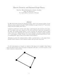
Some values <strong>of</strong> π(x) are given in Table 1.1, and Figures 1.1 and 1.2 contain<br />
graphs <strong>of</strong> π(x). These graphs look like straight lines, which maybe bend<br />
down slightly.<br />
Gauss had a lifelong love <strong>of</strong> enumerating primes. Eventually he computed<br />
π(3000000), though the author doesn’t know whether or not Gauss got the<br />
right answer, which is 216816. Gauss conjectured the following asymptotic<br />
formula for π(x), which was later proved independently by Hadamard and<br />
Vallée Poussin in 1896 (but will not be proved in this book):
18 1. Prime <strong>Number</strong>s<br />
y<br />
180<br />
Graph <strong>of</strong> π(x)<br />
100<br />
(200, 46)<br />
(100, 25)<br />
100<br />
FIGURE 1.1. Graph <strong>of</strong> π(x) for x < 1000<br />
(900, 154) (1000, 168)<br />
900<br />
x<br />
TABLE 1.2. Comparison <strong>of</strong> π(x) and x/(log(x) − 1)<br />
x π(x) x/(log(x) − 1) (approx)<br />
1000 168 169.2690290604408165186256278<br />
2000 303 302.9888734545463878029800994<br />
3000 430 428.1819317975237043747385740<br />
4000 550 548.3922097278253264133400985<br />
5000 669 665.1418784486502172369455815<br />
6000 783 779.2698885854778626863677374<br />
7000 900 891.3035657223339974352567759<br />
8000 1007 1001.602962794770080754784281<br />
9000 1117 1110.428422963188172310675011<br />
10000 1229 1217.976301461550279200775705<br />
Theorem 1.2.8 (Prime <strong>Number</strong> Theorem). The function π(x) is<br />
asymptotic to x/ log(x), in the sense that<br />
lim<br />
x→∞<br />
π(x)<br />
x/ log(x) = 1.<br />
We do nothing more here than motivate this deep theorem with a few<br />
further numerical observations.<br />
The theorem implies that<br />
so for any a,<br />
lim<br />
x→∞<br />
lim π(x)/x = lim 1/ log(x) = 0,<br />
x→∞ x→∞<br />
π(x)<br />
x/(log(x) − a) = lim<br />
x→∞<br />
π(x)<br />
x/ log(x) − aπ(x) = 1.<br />
x<br />
Thus x/(log(x)−a) is also asymptotic to π(x) for any a. See [CP01, §1.1.5]<br />
for a discussion <strong>of</strong> why a = 1 is the best choice. Table 1.2 compares π(x)<br />
and x/(log(x) − 1) for several x < 10000.<br />
As <strong>of</strong> 2004, the record for counting primes appears to be<br />
π(4 · 10 22 ) = 783964159847056303858.<br />
The computation <strong>of</strong> π(4 · 10 22 ) reportedly took ten months on a 350 Mhz<br />
Pentium II (see [GS02] for more details).
1.2 The Sequence <strong>of</strong> Prime <strong>Number</strong>s 19<br />
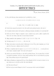
π(x)<br />
650<br />
1000 2000 3000 4000 5000 6000 7000 8000<br />
x<br />
9000 10000<br />
π(x)<br />
4800<br />
x<br />
10000 20000 30000 40000 50000 60000 70000 80000 90000 100000<br />
FIGURE 1.2. Graphs <strong>of</strong> π(x) for x < 10000 and x < 100000<br />
For the reader familiar with complex analysis, we mention a connection<br />
between π(x) and the Riemann Hypothesis. The Riemann zeta function<br />
ζ(s) is a complex analytic function on C \ {1} that extends the function<br />
defined on a right half plane by ∑ ∞<br />
n=1 n−s . The Riemann Hypothesis is<br />
the conjecture that the zeros in C <strong>of</strong> ζ(s) with positive real part lie on the<br />
line Re(s) = 1/2. This conjecture is one <strong>of</strong> the Clay Math Institute million<br />
dollar millennium prize problems [Cla].<br />
According to [CP01, §1.4.1], the Riemann Hypothesis is equivalent to the<br />
conjecture that<br />
Li(x) =<br />
∫ x<br />
2<br />
1<br />
log(t) dt<br />
is a “good” approximation to π(x), in the following precise sense:<br />
Conjecture 1.2.9 (Equivalent to the Riemann Hypothesis).<br />
For all x ≥ 2.01,<br />
|π(x) − Li(x)| ≤ √ x log(x).<br />
If x = 2, then π(2) = 1 and Li(2) = 0, but √ 2 log(2) = 0.9802 . . ., so the<br />
inequality is not true for x ≥ 2, but 2.01 is big enough. We will do nothing<br />
more to explain this conjecture, and settle for one numerical example.<br />
Example 1.2.10. Let x = 4 · 10 22 . Then<br />
π(x) = 783964159847056303858,<br />
Li(x) = 783964159852157952242.7155276025801473 . . . ,<br />
|π(x) − Li(x)| = 5101648384.71552760258014 . . . ,<br />
√ x log(x) = 10408633281397.77913344605 . . . ,<br />
x/(log(x) − 1) = 783650443647303761503.5237113087392967 . . . .<br />
One <strong>of</strong> the best popular article on the prime number theorem and the<br />
Riemann hypothesis is [Zag75].
20 1. Prime <strong>Number</strong>s<br />
1.3 Exercises<br />
1.1 Compute the greatest common divisor gcd(455, 1235) by hand.<br />
1.2 Use the Sieve <strong>of</strong> Eratosthenes to make a list <strong>of</strong> all primes up to 100.<br />
1.3 Prove that there are infinitely many primes <strong>of</strong> the form 6x − 1.<br />
π(x)<br />
1.4 Use Theorem 1.2.8 to deduce that lim<br />
x→∞ x = 0.
2<br />
The Ring <strong>of</strong> Integers Modulo n<br />
This is page 21<br />
Printer: Opaque this<br />
This chapter is about the ring Z/nZ <strong>of</strong> integers modulo n. First we discuss<br />
when linear equations modulo n have a solution, then introduce the Euler ϕ<br />
function and prove Fermat’s Little Theorem and Wilson’s theorem. Next<br />
we prove the Chinese Remainer Theorem, which addresses simultaneous<br />
solubility <strong>of</strong> several linear equations modulo coprime moduli. With these<br />
theoretical foundations in place, in Section 2.3 we introduce algorithms<br />
for doing interesting computations modulo n, including computing large<br />
powers quickly, and solving linear equations. We finish with a very brief<br />
discussion <strong>of</strong> finding prime numbers using arithmetic modulo n.<br />
2.1 Congruences Modulo n<br />
In this section we define the ring Z/nZ <strong>of</strong> integers modulo n, introduce<br />
the Euler ϕ-function, and relate it to the multiplicative order <strong>of</strong> certain<br />
elements <strong>of</strong> Z/nZ.<br />
If a, b ∈ Z and n ∈ N, we say that a is congruent to b modulo n if n | a−b,<br />
and write a ≡ b (mod n). Let nZ = (n) be the ideal <strong>of</strong> Z generated by n.<br />
Definition 2.1.1 (Integers Modulo n). The ring <strong>of</strong> integers modulo n<br />
is the quotient ring Z/nZ <strong>of</strong> equivalence classes <strong>of</strong> integers modulo n. It is<br />
equipped with its natural ring structure:<br />
(a + nZ) + (b + nZ) = (a + b) + nZ<br />
(a + nZ) · (b + nZ) = (a · b) + nZ.
22 2. The Ring <strong>of</strong> Integers Modulo n<br />
Example 2.1.2. For example,<br />
Z/3Z = {{. . . , −3, 0, 3, . . .}, {. . . , −2, 1, 4, . . .}, {. . . , −1, 2, 5, . . .}}<br />
We use the notation Z/nZ because Z/nZ is the quotient <strong>of</strong> the ring Z<br />
by the ideal nZ <strong>of</strong> multiples <strong>of</strong> n. Because Z/nZ is the quotient <strong>of</strong> a ring<br />
by an ideal, the ring structure on Z induces a ring structure on Z/nZ. We<br />
<strong>of</strong>ten let a or a (mod n) denote the equivalence class a + nZ <strong>of</strong> a. If p is a<br />
prime, then Z/pZ is a field (see Exercise 2.11).<br />
We call the natural reduction map Z → Z/nZ, which sends a to a + nZ,<br />
reduction modulo n. We also say that a is a lift <strong>of</strong> a + nZ. Thus, e.g., 7 is<br />
a lift <strong>of</strong> 1 mod 3, since 7 + 3Z = 1 + 3Z.<br />
We can use that arithmetic in Z/nZ is well defined is to derive tests for<br />
divisibility by n (see Exercise 2.7).<br />
Proposition 2.1.3. A number n ∈ Z is divisible by 3 if and only if the<br />
sum <strong>of</strong> the digits <strong>of</strong> n is divisible by 3.<br />
Pro<strong>of</strong>. Write<br />
n = a + 10b + 100c + · · · ,<br />
where the digits <strong>of</strong> n are a, b, c, etc. Since 10 ≡ 1 (mod 3),<br />
n = a + 10b + 100c + · · · ≡ a + b + c + · · · (mod 3),<br />
from which the proposition follows.<br />
2.1.1 Linear Equations Modulo n<br />
In this section, we are concerned with how to decide whether or not a linear<br />
equation <strong>of</strong> the form ax ≡ b (mod n) has a solution modulo n. Algorithms<br />
for computing solutions to ax ≡ b (mod n) are the topic <strong>of</strong> Section 2.3.<br />
First we prove a proposition that gives a criterion under which one can<br />
cancel a quantity from both sides <strong>of</strong> a congruence.<br />
Proposition 2.1.4 (Cancellation). If gcd(c, n) = 1 and<br />
ac ≡ bc<br />
(mod n),<br />
then a ≡ b (mod n).<br />
Pro<strong>of</strong>. By definition<br />
n | ac − bc = (a − b)c.<br />
Since gcd(n, c) = 1, it follows from Theorem 1.1.5 that n | a − b, so<br />
a ≡ b<br />
(mod n),<br />
as claimed.
2.1 Congruences Modulo n 23<br />
When a has a multiplicative inverse a ′ in Z/nZ (i.e., aa ′ ≡ 1 (mod n))<br />
then the equation ax ≡ b (mod n) has a unique solution x ≡ a ′ b (mod n)<br />
modulo n. Thus, it is <strong>of</strong> interest to determine the units in Z/nZ, i.e., the<br />
elements which have a multiplicative inverse.<br />
We will use complete sets <strong>of</strong> residues to prove that the units in Z/nZ<br />
are exactly the a ∈ Z/nZ such that gcd(ã, n) = 1 for any lift ã <strong>of</strong> a to Z<br />
(it doesn’t matter which lift).<br />
Definition 2.1.5 (Complete Set <strong>of</strong> Residues). We call a subset R ⊂ Z<br />
<strong>of</strong> size n whose reductions modulo n are pairwise distinct a complete set <strong>of</strong><br />
residues modulo n. In other words, a complete set <strong>of</strong> residues is a choice <strong>of</strong><br />
representative for each equivalence class in Z/nZ.<br />
For example,<br />
R = {0, 1, 2, . . . , n − 1}<br />
is a complete set <strong>of</strong> residues modulo n. When n = 5, R = {0, 1, −1, 2, −2}<br />
is a complete set <strong>of</strong> residues.<br />
Lemma 2.1.6. If R is a complete set <strong>of</strong> residues modulo n and a ∈ Z with<br />
gcd(a, n) = 1, then aR = {ax : x ∈ R} is also a complete set <strong>of</strong> residues<br />
modulo n.<br />
Pro<strong>of</strong>. If ax ≡ ax ′ (mod n) with x, x ′ ∈ R, then Proposition 2.1.4 implies<br />
that x ≡ x ′ (mod n). Because R is a complete set <strong>of</strong> residues, this implies<br />
that x = x ′ . Thus the elements <strong>of</strong> aR have distinct reductions modulo n. It<br />
follows, since #aR = n, that aR is a complete set <strong>of</strong> residues modulo n.<br />
Proposition 2.1.7 (Units). If gcd(a, n) = 1, then the equation ax ≡ b<br />
(mod n) has a solution, and that solution is unique modulo n.<br />
Pro<strong>of</strong>. Let R be a complete set <strong>of</strong> residues modulo n, so there is a unique<br />
element <strong>of</strong> R that is congruent to b modulo n. By Lemma 2.1.6, aR is also<br />
a complete set <strong>of</strong> residues modulo n, so there is a unique element ax ∈ aR<br />
that is congruent to b modulo n, and we have ax ≡ b (mod n).<br />
Algebraically, this proposition asserts that if gcd(a, n) = 1, then the map<br />
Z/nZ → Z/nZ given by left multiplication by a is a bijection.<br />
Example 2.1.8. Consider the equation 2x ≡ 3 (mod 7), and the complete<br />
set R = {0, 1, 2, 3, 4, 5, 6} <strong>of</strong> coset representatives. We have<br />
so 2 · 5 ≡ 3 (mod 7).<br />
2R = {0, 2, 4, 6, 8 ≡ 1, 10 ≡ 3, 12 ≡ 5},<br />
When gcd(a, n) ≠ 1, then the equation ax ≡ b (mod n) may or may<br />
not have a solution. For example, 2x ≡ 1 (mod 4) has no solution, but<br />
2x ≡ 2 (mod 4) does, and in fact it has more than one mod 4 (x = 1<br />
and x = 3). Generalizing Proposition 2.1.7, we obtain the following more<br />
general criterion for solvability.
24 2. The Ring <strong>of</strong> Integers Modulo n<br />
Proposition 2.1.9 (Solvability). The equation ax ≡ b (mod n) has a<br />
solution if and only if gcd(a, n) divides b.<br />
Pro<strong>of</strong>. Let g = gcd(a, n). If there is a solution x to the equation ax ≡ b<br />
(mod n), then n | (ax − b). Since g | n and g | a, it follows that g | b.<br />
Conversely, suppose that g | b. Then n | (ax − b) if and only if<br />
(<br />
n a<br />
g | g x − b )<br />
.<br />
g<br />
Thus ax ≡ b (mod n) has a solution if and only if a g x ≡ b g<br />
(mod n g ) has<br />
a solution. Since gcd(a/g, n/g) = 1, Proposition 2.1.7 implies this latter<br />
equation does have a solution.<br />
In Chapter 4 we will study quadratic reciprocity, which gives a nice<br />
criterion for whether or not a quadratic equation modulo n has a solution.<br />
2.1.2 Fermat’s Little Theorem<br />
The group <strong>of</strong> units (Z/nZ) ∗ <strong>of</strong> the ring Z/nZ will be <strong>of</strong> great interest<br />
to us. Each element <strong>of</strong> this group has an order, and Lagrange’s theorem<br />
from group theory implies that each element <strong>of</strong> (Z/nZ) ∗ has order that<br />
divides the order <strong>of</strong> (Z/nZ) ∗ . In elementary number theory this fact goes<br />
by the monicker “Fermat’s Little Theorem”, and we reprove it from basic<br />
principles in this section.<br />
Definition 2.1.10 (Order <strong>of</strong> an Element). Let n ∈ N and x ∈ Z and<br />
suppose that gcd(x, n) = 1. The order <strong>of</strong> x modulo n is the smallest m ∈ N<br />
such that<br />
x m ≡ 1<br />
(mod n).<br />
To show that the definition makes sense, we verify that such an m exists.<br />
Consider x, x 2 , x 3 , . . . modulo n. There are only finitely many residue classes<br />
modulo n, so we must eventually find two integers i, j with i < j such that<br />
x j ≡ x i<br />
(mod n).<br />
Since gcd(x, n) = 1, Proposition 2.1.4 implies that we can cancel x’s and<br />
conclude that<br />
x j−i ≡ 1<br />
(mod n).<br />
Definition 2.1.11 (Euler’s phi-function). For n ∈ N, let<br />
ϕ(n) = #{a ∈ N : a ≤ n and gcd(a, n) = 1}.
2.1 Congruences Modulo n 25<br />
For example,<br />
ϕ(1) = #{1} = 1,<br />
ϕ(2) = #{1} = 1,<br />
ϕ(5) = #{1, 2, 3, 4} = 4,<br />
ϕ(12) = #{1, 5, 7, 11} = 4.<br />
Also, if p is any prime number then<br />
ϕ(p) = #{1, 2, . . . , p − 1} = p − 1.<br />
In Section 2.2.1, we will prove that ϕ is a multiplicative function. This will<br />
yield an easy way to compute ϕ(n) in terms <strong>of</strong> the prime factorization <strong>of</strong> n.<br />
Theorem 2.1.12 (Fermat’s Little Theorem). If gcd(x, n) = 1, then<br />
x ϕ(n) ≡ 1<br />
(mod n).<br />
Pro<strong>of</strong>. As mentioned above, Fermat’s Little Theorem has the following<br />
group-theoretic interpretation. The set <strong>of</strong> units in Z/nZ is a group<br />
(Z/nZ) ∗ = {a ∈ Z/nZ : gcd(a, n) = 1}.<br />
which has order ϕ(n). The theorem then asserts that the order <strong>of</strong> an element<br />
<strong>of</strong> (Z/nZ) ∗ divides the order ϕ(n) <strong>of</strong> (Z/nZ) ∗ . This is a special case <strong>of</strong> the<br />
more general fact (Lagrange’s theorem) that if G is a finite group and<br />
g ∈ G, then the order <strong>of</strong> g divides the cardinality <strong>of</strong> G.<br />
We now give an elementary pro<strong>of</strong> <strong>of</strong> the theorem. Let<br />
P = {a : 1 ≤ a ≤ n and gcd(a, n) = 1}.<br />
In the same way that we proved Lemma 2.1.6, we see that the reductions<br />
modulo n <strong>of</strong> the elements <strong>of</strong> xP are the same as the reductions <strong>of</strong> the<br />
elements <strong>of</strong> P . Thus<br />
∏<br />
≡<br />
a∈P(xa) ∏ a (mod n),<br />
a∈P<br />
since the products are over the same numbers modulo n. Now cancel the<br />
a’s on both sides to get<br />
x #P ≡ 1<br />
(mod n),<br />
as claimed.
26 2. The Ring <strong>of</strong> Integers Modulo n<br />
2.1.3 Wilson’s Theorem<br />
The following characterization <strong>of</strong> prime numbers, from the 1770s, is called<br />
“Wilson’s Theorem”, though it was first proved by Lagrange.<br />
Proposition 2.1.13 (Wilson’s Theorem). An integer p > 1 is prime if<br />
and only if (p − 1)! ≡ −1 (mod p).<br />
For example, if p = 3, then (p − 1)! = 2 ≡ −1 (mod 3). If p = 17, then<br />
But if p = 15, then<br />
(p − 1)! = 20922789888000 ≡ −1 (mod 17).<br />
(p − 1)! = 87178291200 ≡ 0 (mod 15),<br />
so 15 is composite. Thus Wilson’s theorem could be viewed as a primality<br />
test, though, from a computational point <strong>of</strong> view, it is probably the least<br />
efficient primality test since computing (n − 1)! takes so many steps.<br />
Pro<strong>of</strong>. The statement is clear when p = 2, so henceforth we assume that<br />
p > 2. We first assume that p is prime and prove that (p − 1)! ≡ −1<br />
(mod p). If a ∈ {1, 2, . . . , p − 1} then the equation<br />
ax ≡ 1 (mod p)<br />
has a unique solution a ′ ∈ {1, 2, . . . , p − 1}. If a = a ′ , then a 2 ≡ 1 (mod p),<br />
so p | a 2 −1 = (a−1)(a+1), so p | (a−1) or p | (a+1), so a ∈ {1, p−1}. We<br />
can thus pair <strong>of</strong>f the elements <strong>of</strong> {2, 3, . . . , p − 2}, each with their inverse.<br />
Thus<br />
2 · 3 · · · · · (p − 2) ≡ 1 (mod p).<br />
Multiplying both sides by p − 1 proves that (p − 1)! ≡ −1 (mod p).<br />
Next we assume that (p − 1)! ≡ −1 (mod p) and prove that p must be<br />
prime. Suppose not, so that p ≥ 4 is a composite number. Let l be a prime<br />
divisor <strong>of</strong> p. Then l < p, so l | (p − 1)!. Also, by assumption,<br />
l | p | ((p − 1)! + 1).<br />
This is a contradiction, because a prime can not divide a number a and<br />
also divide a + 1, since it would then have to divide (a + 1) − a = 1.<br />
Example 2.1.14. We illustrate the key step in the above pro<strong>of</strong> in the case<br />
p = 17. We have<br />
2·3 · · · 15 = (2·9)·(3·6)·(4·13)·(5·7)·(8·15)·(10·12)·(14·11) ≡ 1 (mod 17),<br />
where we have paired up the numbers a, b for which ab ≡ 1 (mod 17).
2.2 The Chinese Remainder Theorem 27<br />
2.2 The Chinese Remainder Theorem<br />
In this section we prove the Chinese Remainder Theorem, which gives conditions<br />
under which a system <strong>of</strong> linear equations is guaranteed to have a<br />
solution. In the 4th century a Chinese mathematician asked the following:<br />
Question 2.2.1. There is a quantity whose number is unknown. Repeatedly<br />
divided by 3, the remainder is 2; by 5 the remainder is 3; and by 7 the<br />
remainder is 2. What is the quantity?<br />
In modern notation, Question 2.2.1 asks us to find a positive integer<br />
solution to the following system <strong>of</strong> three equations:<br />
x ≡ 2 (mod 3)<br />
x ≡ 3 (mod 5)<br />
x ≡ 2 (mod 7)<br />
The Chinese Remainder Theorem asserts that a solution exists, and the<br />
pro<strong>of</strong> gives a method to find one. (See Section 2.3 for the necessary algorithms.)<br />
Theorem 2.2.2 (Chinese Remainder Theorem). Let a, b ∈ Z and<br />
n, m ∈ N such that gcd(n, m) = 1. Then there exists x ∈ Z such that<br />
x ≡ a<br />
x ≡ b<br />
(mod m),<br />
(mod n).<br />
Moreover x is unique modulo mn.<br />
Pro<strong>of</strong>. If we can solve for t in the equation<br />
a + tm ≡ b<br />
(mod n),<br />
then x = a + tm will satisfy both congruences. To see that we can solve,<br />
subtract a from both sides and use Proposition 2.1.7 together with our<br />
assumption that gcd(n, m) = 1 to see that there is a solution.<br />
For uniqueness, suppose that x and y solve both congruences. Then z =<br />
x − y satisfies z ≡ 0 (mod m) and z ≡ 0 (mod n), so m | z and n | z. Since<br />
gcd(n, m) = 1, it follows that nm | z, so x ≡ y (mod nm).<br />
Algorithm 2.2.3 (Chinese Remainder Theorem). Given coprime integers<br />
m and n and integers a and b, this algorithm find an integer x such<br />
that x ≡ a (mod m) and x ≡ b (mod n).<br />
1. [Extended GCD] Use Algorithm 2.3.3 below to find integers c, d such<br />
that cm + dn = 1.<br />
2. [Answer] Output x = a + (b − a)cm and terminate.
28 2. The Ring <strong>of</strong> Integers Modulo n<br />
Pro<strong>of</strong>. Since c ∈ Z, we have x ≡ a (mod m), and using that cm + dn = 1,<br />
we have a + (b − a)cm ≡ a + (b − a) ≡ b (mod n).<br />
Now we can answer Question 2.2.1. First, we use Theorem 2.2.2 to find<br />
a solution to the pair <strong>of</strong> equations<br />
x ≡ 2 (mod 3),<br />
x ≡ 3 (mod 5).<br />
Set a = 2, b = 3, m = 3, n = 5. Step 1 is to find a solution to t · 3 ≡ 3 − 2<br />
(mod 5). A solution is t = 2. Then x = a + tm = 2 + 2 · 3 = 8. Since any x ′<br />
with x ′ ≡ x (mod 15) is also a solution to those two equations, we can<br />
solve all three equations by finding a solution to the pair <strong>of</strong> equations<br />
x ≡ 8 (mod 15)<br />
x ≡ 2 (mod 7).<br />
Again, we find a solution to t · 15 ≡ 2 − 8 (mod 7). A solution is t = 1, so<br />
x = a + tm = 8 + 15 = 23.<br />
Note that there are other solutions. Any x ′ ≡ x (mod 3 · 5 · 7) is also a<br />
solution; e.g., 23 + 3 · 5 · 7 = 128.<br />
2.2.1 Multiplicative Functions<br />
Definition 2.2.4 (Multiplicative Function). A function f : N → Z is<br />
multiplicative if, whenever m, n ∈ N and gcd(m, n) = 1, we have<br />
f(mn) = f(m) · f(n).<br />
Recall from Definition 2.1.11 that the Euler ϕ-function is<br />
ϕ(n) = #{a : 1 ≤ a ≤ n and gcd(a, n) = 1}.<br />
Lemma 2.2.5. Suppose that m, n ∈ N and gcd(m, n) = 1. Then the map<br />
ψ : (Z/mnZ) ∗ → (Z/mZ) ∗ × (Z/nZ) ∗ . (2.2.1)<br />
defined by<br />
is a bijection.<br />
ψ(c) = (c mod m, c mod n)<br />
Pro<strong>of</strong>. We first show that ψ is injective. If ψ(c) = ψ(c ′ ), then m | c−c ′ and<br />
n | c − c ′ , so nm | c − c ′ because gcd(n, m) = 1. Thus c = c ′ as elements <strong>of</strong><br />
(Z/mnZ) ∗ .<br />
Next we show that ψ is surjective. Given a and b with gcd(a, m) = 1<br />
and gcd(b, n) = 1, Theorem 2.2.2 implies that there exists c with c ≡ a<br />
(mod m) and c ≡ b (mod n). We may assume that 1 ≤ c ≤ nm, and<br />
since gcd(a, m) = 1 and gcd(b, n) = 1, we must have gcd(c, nm) = 1. Thus<br />
ψ(c) = (a, b).
2.3 Quickly Computing Inverses and Huge Powers 29<br />
Proposition 2.2.6 (Multiplicativity <strong>of</strong> ϕ). The function ϕ is multiplicative.<br />
Pro<strong>of</strong>. The map ψ <strong>of</strong> Lemma 2.2.5 is a bijection, so the set on the left in<br />
(2.2.1) has the same size as the product set on the right in (2.2.1). Thus<br />
ϕ(mn) = ϕ(m) · ϕ(n).<br />
The proposition is helpful in computing ϕ(n), at least if we assume we can<br />
compute the factorization <strong>of</strong> n (see Section 3.3.1 for a connection between<br />
factoring n and computing ϕ(n)). For example,<br />
Also, for n ≥ 1, we have<br />
ϕ(12) = ϕ(2 2 ) · ϕ(3) = 2 · 2 = 4.<br />
ϕ(p n ) = p n − pn p = pn − p n−1 = p n−1 (p − 1), (2.2.2)<br />
since ϕ(p n ) is the number <strong>of</strong> numbers less than p n minus the number <strong>of</strong><br />
those that are divisible by p. Thus, e.g.,<br />
ϕ(389 · 11 2 ) = 388 · (11 2 − 11) = 388 · 110 = 42680.<br />
2.3 Quickly Computing Inverses and Huge Powers<br />
This section is about how to solve the equation ax ≡ 1 (mod n) when<br />
we know it has a solution, and how to efficiently compute a m (mod n).<br />
We also discuss a simple probabilistic primality test that relies on our<br />
ability to compute a m (mod n) quickly. All three <strong>of</strong> these algorithms are<br />
<strong>of</strong> fundamental importance to the cryptography algorithms <strong>of</strong> Chapter 3.<br />
2.3.1 How to Solve ax ≡ 1 (mod n)<br />
Suppose a, n ∈ N with gcd(a, n) = 1. Then by Proposition 2.1.7 the equation<br />
ax ≡ 1 (mod n) has a unique solution. How can we find it?<br />
Proposition 2.3.1 (Extended Euclidean representation). Suppose<br />
a, b ∈ Z and let g = gcd(a, b). Then there exists x, y ∈ Z such that<br />
ax + by = g.<br />
Remark 2.3.2. If e = cg is a multiple <strong>of</strong> g, then cax + cby = cg = e, so<br />
e = (cx)a + (cy)b can also be written in terms <strong>of</strong> a and b.
30 2. The Ring <strong>of</strong> Integers Modulo n<br />
Pro<strong>of</strong> <strong>of</strong> Proposition 2.3.1. Let g = gcd(a, b). Then gcd(a/d, b/d) = 1, so<br />
by Proposition 2.1.9 the equation<br />
a<br />
(mod<br />
g · x ≡ 1 b )<br />
(2.3.1)<br />
g<br />
has a solution x ∈ Z. Multiplying (2.3.1) through by g yields ax ≡ g<br />
(mod b), so there exists y such that b · (−y) = ax − g. Then ax + by = g,<br />
as required.<br />
Given a, b and g = gcd(a, b), our pro<strong>of</strong> <strong>of</strong> Proposition 2.3.1 gives a way to<br />
explicitly find x, y such that ax+by = g, assuming one knows an algorithm<br />
to solve linear equations modulo n. Since we do not know such an algorithm,<br />
we now discuss a way to explicitly find x and y. This algorithm will in fact<br />
enable us to solve linear equations modulo n—to solve ax ≡ 1 (mod n)<br />
when gcd(a, n) = 1, use the algorithm below to find x and y such that<br />
ax + ny = 1. Then ax ≡ 1 (mod n).<br />
Suppose a = 5 and b = 7. The steps <strong>of</strong> Algorithm 1.1.12 to compute<br />
gcd(5, 7) are, as follows. Here we underlying, because it clarifies the subsequent<br />
back substitution we will use to find x and y.<br />
7 = 1 · 5 + 2 so 2 = 7 − 5<br />
5 = 2 · 2 + 1 so 1 = 5 − 2 · 2 = 5 − 2(7 − 5) = 3 · 5 − 2 · 7<br />
On the right, we have back-substituted in order to write each partial remainder<br />
as a linear combination <strong>of</strong> a and b. In the last step, we obtain<br />
gcd(a, b) as a linear combination <strong>of</strong> a and b, as desired.<br />
That example was not too complicated, so we try another one. Let a =<br />
130 and b = 61. We have<br />
130 = 2 · 61 + 8 8 = 130 − 2 · 61<br />
61 = 7 · 8 + 5 5 = −7 · 130 + 15 · 61<br />
8 = 1 · 5 + 3 3 = 8 · 130 − 17 · 61<br />
5 = 1 · 3 + 2 2 = −15 · 130 + 32 · 61<br />
3 = 1 · 2 + 1 1 = 23 · 130 − 49 · 61<br />
Thus x = 23 and y = −49 is a solution to 130x + 61y = 1.<br />
Algorithm 2.3.3 (Extended Euclidean Algorithm). Suppose a and b<br />
are integers and let g = gcd(a, b). This algorithm finds d, x and y such that<br />
ax + by = g. We describe only the steps when a > b ≥ 0, since one can easily<br />
reduce to this case.<br />
1. [Initialize] Set x = 1, y = 0, r = 0, s = 1.<br />
2. [Finished?] If b = 0, set g = a and terminate.
2.3 Quickly Computing Inverses and Huge Powers 31<br />
3. [Quotient and Remainder] Use Algorithm 1.1.11 to write a = qb+c with<br />
0 ≤ c < b.<br />
4. [Shift] Set (a, b, r, s, x, y) = (b, c, x − qr, y − qs, r, s) and go to step 2.<br />
Pro<strong>of</strong>. This algorithm is the same as Algorithm 1.1.12, except that we keep<br />
track <strong>of</strong> extra variables x, y, r, s, so it terminates and when it terminates<br />
d = gcd(a, b). We omit the rest <strong>of</strong> the inductive pro<strong>of</strong> that the algorithm<br />
is correct, and instead refer the reader to [Knu97, §1.2.1] which contains a<br />
detailed pro<strong>of</strong> in the context <strong>of</strong> a discussion <strong>of</strong> how one writes mathematical<br />
pro<strong>of</strong>s.<br />
Algorithm 2.3.4 (Inverse Modulo n). Suppose a and n are integers and<br />
gcd(a, n) = 1. This algorithm finds an x such that ax ≡ 1 (mod n).<br />
1. [Compute Extended GCD] Use Algorithm 2.3.3 to compute integers x, y<br />
such that ax + ny = gcd(a, n) = 1.<br />
2. [Finished] Output x.<br />
Pro<strong>of</strong>. Reduce ax+ny = 1 modulo n to see that x satisfies ax ≡ 1 (mod n).<br />
See Section 7.2.1 for implementations <strong>of</strong> Algorithms 2.3.3 and 2.3.4.<br />
Example 2.3.5. Solve 17x ≡ 1 (mod 61). First, we use Algorithm 2.3.3 to<br />
find x, y such that 17x + 61y = 1:<br />
61 = 3 · 17 + 10 10 = 61 − 3 · 17<br />
17 = 1 · 10 + 7 7 = −61 + 4 · 17<br />
10 = 1 · 7 + 3 3 = 2 · 61 − 7 · 17<br />
3 = 2 · 3 + 1 1 = −5 · 61 + 18 · 17<br />
Thus 17 · 18 + 61 · (−5) = 1 so x = 18 is a solution to 17x ≡ 1 (mod 61).<br />
2.3.2 How to Compute a m (mod n)<br />
Let a and n be integers, and m a nonnegative integer. In this section we describe<br />
an efficient algorithm to compute a m (mod n). For the cryptography<br />
applications in Chapter 3, m will have hundreds <strong>of</strong> digits.<br />
The naive approach to computing a m (mod n) is to simply compute<br />
a m = a · a · · · a (mod n) by repeatedly multiplying by a and reducing modulo<br />
m. Note that after each arithmetic operation is completed, we reduce<br />
the result modulo n so that the sizes <strong>of</strong> the numbers involved do not get<br />
too large. Nonetheless, this algorithm is horribly inefficient because it takes<br />
m − 1 multiplications, which is huge if m has hundreds <strong>of</strong> digits.<br />
A much more efficient algorithm for computing a m (mod n) involves<br />
writing m in binary, then expressing a m as a product <strong>of</strong> expressions a 2i , for
32 2. The Ring <strong>of</strong> Integers Modulo n<br />
various i. These latter expressions can be computed by repeatedly squaring<br />
a 2i . This more clever algorithm is not “simpler”, but it is vastly more<br />
efficient since the number <strong>of</strong> operations needed grows with the number <strong>of</strong><br />
binary digits <strong>of</strong> m, whereas with the naive algorithm above the number <strong>of</strong><br />
operations is m − 1.<br />
Algorithm 2.3.6 (Write a number in binary). Let m be a nonnegative<br />
integer. This algorithm writes m in binary, so it finds ε i ∈ {0, 1} such that<br />
m = ∑ r<br />
i=0 ε i2 i with each ε i ∈ {0, 1}.<br />
1. [Initialize] Set i = 0.<br />
2. [Finished?] If m = 0, terminate.<br />
3. [Digit] If m is odd, set ε i = 1, otherwise ε i = 0. Increment i.<br />
4. [Divide by 2] Set m = ⌊ ⌋<br />
m<br />
2 , the greatest integer ≤ m/2. Goto step 2.<br />
Algorithm 2.3.7 (Compute Power). Let a and n be integers and m a<br />
nonnegative integer. This algorithm computes a m modulo n.<br />
1. [Write in Binary] Write m in binary using Algorithm 2.3.6, so a m =<br />
(mod n).<br />
∏<br />
ε i=1 a2i<br />
2. [Compute Powers] Compute a, a 2 , a 22 = (a 2 ) 2 , a 23 = (a 22 ) 2 , etc., up<br />
to a 2r , where r + 1 is the number <strong>of</strong> binary digits <strong>of</strong> m.<br />
3. [Multiply Powers] Multiply together the a 2i such that ε i = 1, always<br />
working modulo n.<br />
See Section 7.2.2 for an implementation <strong>of</strong> Algorithms 2.3.6 and 2.3.7.<br />
We can compute the last 2 digits <strong>of</strong> 6 91 , by finding 6 91 (mod 100). Make a<br />
table whose first column, labeled i, contains 0, 1, 2, etc. The second column,<br />
labeled m, is got by dividing the entry above it by 2 and taking the integer<br />
part <strong>of</strong> the result. The third column, labeled ε i , records whether or not the<br />
second column is odd. The fourth column is computed by squaring, modulo<br />
n = 100, the entry above it.<br />
We have<br />
i m ε i 6 2i mod 100<br />
0 91 1 6<br />
1 45 1 36<br />
2 22 0 96<br />
3 11 1 16<br />
4 5 1 56<br />
5 2 0 36<br />
6 1 1 96<br />
6 91 ≡ 6 26 · 6 24 · 6 23 · 6 2 · 6 ≡ 96 · 56 · 16 · 36 · 6 ≡ 56 (mod 100).<br />
That is easier than multiplying 6 by itself 91 times.
2.4 Finding Primes 33<br />
Remark 2.3.8. Alternatively, we could simplify the computation using Theorem<br />
2.1.12. By that theorem, 6 ϕ(100) ≡ 1 (mod 100), so since ϕ(100) =<br />
ϕ(2 2 · 5 2 ) = (2 2 − 2) · (5 2 − 5) = 40, we have 6 91 ≡ 6 11 (mod 100).<br />
2.4 Finding Primes<br />
Theorem 2.4.1 (Pseudoprimality). An integer p > 1 is prime if and<br />
only if for every a ≢ 0 (mod p),<br />
a p−1 ≡ 1<br />
(mod p).<br />
Pro<strong>of</strong>. If p is prime, then the statement follows from Proposition 2.1.13.<br />
If p is composite, then there is a divisor a <strong>of</strong> p with a ≠ 1, p. If a p−1 ≡ 1<br />
(mod p), then p | a p−1 − 1. Since a | p, we have a | a p−1 − 1 hence a | 1, a<br />
contradiction.<br />
Suppose n ∈ N. Using this theorem and Algorithm 2.3.7, we can either<br />
quickly prove that n is not prime, or convince ourselves that n is likely<br />
prime (but not quickly prove that n is prime). For example, if 2 n−1 ≢ 1<br />
(mod n), then we have proved that n is not prime. On the other hand,<br />
if a n−1 ≡ 1 (mod n) for a few a, it “seems likely” that n is prime, and<br />
we loosely refer to such a number that seems prime for several bases as a<br />
pseudoprime.<br />
There are composite numbers n (called Carmichael numbers) with the<br />
amazing property that a n−1 ≡ 1 (mod n) for all a with gcd(a, n) = 1. The<br />
first Carmichael number is 561, and it is a theorem that there are infinitely<br />
many such numbers ([AGP94]).<br />
Example 2.4.2. Is p = 323 prime? We compute 2 322 (mod 323). Making a<br />
table as above, we have<br />
Thus<br />
i m ε i 2 2i mod 323<br />
0 322 0 2<br />
1 161 1 4<br />
2 80 0 16<br />
3 40 0 256<br />
4 20 0 290<br />
5 10 0 120<br />
6 5 1 188<br />
7 2 0 137<br />
8 1 1 35<br />
2 322 ≡ 4 · 188 · 35 ≡ 157 (mod 323),<br />
so 323 is not prime, though this computation gives no information about<br />
323 factors as a product <strong>of</strong> primes. In fact, one finds that 323 = 17 · 19.
34 2. The Ring <strong>of</strong> Integers Modulo n<br />
It’s possible to easily prove that a large number is composite, but the<br />
pro<strong>of</strong> does not easily yield a factorization. For example if<br />
n = 95468093486093450983409583409850934850938459083,<br />
then 2 n−1 ≢ 1 (mod n), so n is composite.<br />
Another practical primality test is the Miller-Rabin test, which has the<br />
property that each time it is run on a number n it either correctly asserts<br />
that the number is definitely not prime, or that it is probably prime, and<br />
the probability <strong>of</strong> correctness goes up with each successive call. For a precise<br />
statement and implementation <strong>of</strong> Miller-Rabin, along with pro<strong>of</strong> <strong>of</strong><br />
correctness, see Section 7.2.4. If Miller-Rabin is called m times on n and<br />
in each case claims that n is probably prime, then one can in a precise<br />
sense bound the probability that n is composite in terms <strong>of</strong> m. For an<br />
implementation <strong>of</strong> Miller-Rabin, see Listing 7.2.9 in Chapter 7.<br />
Until recently it was an open problem to give an algorithm (with pro<strong>of</strong>)<br />
that decides whether or not any integer is prime in time bounded by a polynomial<br />
in the number <strong>of</strong> digits <strong>of</strong> the integer. Agrawal, Kayal, and Saxena<br />
recently found the first polynomial-time primality test (see [AKS02]). We<br />
will not discuss their algorithm further, because for our applications to<br />
cryptography Miller-Rabin or pseudoprimality tests will be sufficient.<br />
2.5 The Structure <strong>of</strong> (Z/pZ) ∗<br />
This section is about the structure <strong>of</strong> the group (Z/pZ) ∗ <strong>of</strong> units modulo<br />
a prime number p. The main result is that this group is always cyclic. We<br />
will use this result later in Chapter 4 in our pro<strong>of</strong> <strong>of</strong> quadratic reciprocity.<br />
Definition 2.5.1 (Primitive root). A primitive root modulo an integer n<br />
is an element <strong>of</strong> (Z/nZ) ∗ <strong>of</strong> order ϕ(n).<br />
We will prove that there is a primitive root modulo every prime p. Since<br />
the unit group (Z/pZ) ∗ has order p−1, this implies that (Z/pZ) ∗ is a cyclic<br />
group, a fact this will be extremely useful, since it completely determines<br />
the structure <strong>of</strong> (Z/pZ) ∗ as an abelian group.<br />
If n is an odd prime power, then there is a primitive root modulo n (see<br />
Exercise 2.25), but there is no primitive root modulo the prime power 2 3 ,<br />
and hence none mod 2 n for n ≥ 3 (see Exercise 2.24).<br />
Section 2.5.1 is the key input to our pro<strong>of</strong> that (Z/pZ) ∗ is cyclic; here<br />
we show that for every divisor d <strong>of</strong> p − 1 there are exactly d elements <strong>of</strong><br />
(Z/pZ) ∗ whose order divides d. We then use this result in Section 2.5.2 to<br />
produce an element <strong>of</strong> (Z/pZ) ∗ <strong>of</strong> order q r when q r is a prime power that<br />
exactly divides p − 1 (i.e., q r divides p − 1, but q r+1 does not divide p − 1),<br />
and multiply together these elements to obtain an element <strong>of</strong> (Z/pZ) ∗ <strong>of</strong><br />
order p − 1.
2.5 The Structure <strong>of</strong> (Z/pZ) ∗ 35<br />
2.5.1 Polynomials over Z/pZ<br />
The polynomials x 2 − 1 has four roots in Z/8Z, namely 1, 3, 5, and 7.<br />
In contrast, the following proposition shows that a polynomial <strong>of</strong> degree d<br />
over a field, such as Z/pZ, can have at most d roots.<br />
Proposition 2.5.2 (Root Bound). Let f ∈ k[x] be a nonzero polynomial<br />
over a field k. Then there are at most deg(f) elements α ∈ k such that<br />
f(α) = 0.<br />
Pro<strong>of</strong>. We prove the proposition by induction on deg(f). The cases in which<br />
deg(f) ≤ 1 are clear. Write f = a n x n + · · · a 1 x + a 0 . If f(α) = 0 then<br />
f(x) = f(x) − f(α)<br />
= a n (x n − α n ) + · · · a 1 (x − α) + a 0 (1 − 1)<br />
= (x − α)(a n (x n−1 + · · · + α n−1 ) + · · · + a 2 (x + α) + a 1 )<br />
= (x − α)g(x),<br />
for some polynomial g(x) ∈ k[x]. Next suppose that f(β) = 0 with β ≠ α.<br />
Then (β − α)g(β) = 0, so, since β − α ≠ 0, we have g(β) = 0. By our<br />
inductive hypothesis, g has at most n − 1 roots, so there are at most n − 1<br />
possibilities for β. It follows that f has at most n roots.<br />
Proposition 2.5.3. Let p be a prime number and let d be a divisor <strong>of</strong><br />
p − 1. Then f = x d − 1 ∈ (Z/pZ)[x] has exactly d roots in Z/pZ.<br />
Pro<strong>of</strong>. Let e = (p − 1)/d. We have<br />
x p−1 − 1 = (x d ) e − 1<br />
= (x d − 1)((x d ) e−1 + (x d ) e−2 + · · · + 1)<br />
= (x d − 1)g(x),<br />
where g ∈ (Z/pZ)[x] and deg(g) = de − d = p − 1 − d. Theorem 2.1.12<br />
implies that x p−1 − 1 has exactly p − 1 roots in Z/pZ, since every nonzero<br />
element <strong>of</strong> Z/pZ is a root! By Proposition 2.5.2, g has at most p − 1 − d<br />
roots and x d − 1 has at most d roots. Since a root <strong>of</strong> (x d − 1)g(x) is a root<br />
<strong>of</strong> either x d − 1 or g(x) and x p−1 − 1 has p − 1 roots, g must have exactly<br />
p − 1 − d roots and x d − 1 must have exactly d roots, as claimed.<br />
We pause to reemphasize that the analogue <strong>of</strong> Proposition 2.5.3 is false<br />
when p is replaced by a composite integer n, since a root mod n <strong>of</strong> a<br />
product <strong>of</strong> two polynomials need not be a root <strong>of</strong> either factor. For example,<br />
f = x 2 − 1 ∈ Z/15Z[x] has the four roots 1, 4, 11, and 14.
36 2. The Ring <strong>of</strong> Integers Modulo n<br />
2.5.2 Existence <strong>of</strong> Primitive Roots<br />
Recall from Section 2.1.2 that the order <strong>of</strong> an element x in a finite group<br />
is the smallest m ≥ 1 such that x m = 1. In this section, we prove that<br />
(Z/pZ) ∗ is cyclic by using the results <strong>of</strong> Section 2.5.1 to produce an element<br />
<strong>of</strong> (Z/pZ) ∗ <strong>of</strong> order d for each prime power divisor d <strong>of</strong> p − 1, and then we<br />
multiply these together to obtain an element <strong>of</strong> order p − 1.<br />
We will use the following lemma to assemble elements <strong>of</strong> each order<br />
dividing p − 1 to produce an element <strong>of</strong> order p − 1.<br />
Lemma 2.5.4. Suppose a, b ∈ (Z/nZ) ∗ have orders r and s, respectively,<br />
and that gcd(r, s) = 1. Then ab has order rs.<br />
Pro<strong>of</strong>. This is a general fact about commuting elements <strong>of</strong> any group; our<br />
pro<strong>of</strong> only uses that ab = ba and nothing special about (Z/nZ) ∗ . Since<br />
(ab) rs = a rs b rs = 1,<br />
the order <strong>of</strong> ab is a divisor <strong>of</strong> rs. Write this divisor as r 1 s 1 where r 1 | r and<br />
s 1 | s. Raise both sides <strong>of</strong> the equation<br />
to the power r 2 = r/r 1 to obtain<br />
a r1s1 b r1s1 = (ab) r1s1 = 1.<br />
a r1r2s1 b r1r2s1 = 1.<br />
Since a r1r2s1 = (a r1r2 ) s1 = 1, we have<br />
b r1r2s1 = 1,<br />
so s | r 1 r 2 s 1 . Since gcd(s, r 1 r 2 ) = gcd(s, r) = 1, it follows that s = s 1 .<br />
Similarly r = r 1 , so the order <strong>of</strong> ab is rs.<br />
Theorem 2.5.5 (Primitive Roots). There is a primitive root modulo<br />
any prime p. In particular, the group (Z/pZ) ∗ is cyclic.<br />
Pro<strong>of</strong>. The theorem is true if p = 2, since 1 is a primitive root, so we may<br />
assume p > 2. Write p − 1 as a product <strong>of</strong> distinct prime powers q ni<br />
i :<br />
p − 1 = q n1<br />
1 qn2 2 · · · qnr r .<br />
By Proposition 2.5.3, the polynomial x qn i<br />
i<br />
the polynomial x qn i −1<br />
i<br />
− 1 has exactly q ni−1<br />
i<br />
(q i − 1) elements a ∈ Z/pZ such that a qn i<br />
i<br />
<strong>of</strong> these elements has order q ni<br />
i<br />
q ni−1<br />
i<br />
an a i <strong>of</strong> order q ni<br />
i<br />
− 1 has exactly q ni<br />
i<br />
roots, and<br />
roots. There are q ni<br />
i − q ni−1<br />
i =<br />
= 1 but a qn i −1<br />
i ≠ 1; each<br />
. Thus for each i = 1, . . . , r, we can choose<br />
. Then, using Lemma 2.5.4 repeatedly, we see that<br />
a = a 1 a 2 · · · a r<br />
has order q n1<br />
1 · · · qnr r = p − 1, so a is a primitive root modulo p.
2.5 The Structure <strong>of</strong> (Z/pZ) ∗ 37<br />
Example 2.5.6. We illustrate the pro<strong>of</strong> <strong>of</strong> Theorem 2.5.5 when p = 13. We<br />
have<br />
p − 1 = 12 = 2 2 · 3.<br />
The polynomial x 4 − 1 has roots {1, 5, 8, 12} and x 2 − 1 has roots {1, 12},<br />
so we may take a 1 = 5. The polynomial x 3 − 1 has roots {1, 3, 9}, and we<br />
set a 2 = 3. Then a = 5 · 3 = 15 ≡ 2 is a primitive root. To verify this, note<br />
that the successive powers <strong>of</strong> 2 (mod 13) are<br />
2, 4, 8, 3, 6, 12, 11, 9, 5, 10, 7, 1.<br />
Example 2.5.7. Theorem 2.5.5 is false if, e.g., p is replaced by a power <strong>of</strong> 2<br />
bigger than 4. For example, the four elements <strong>of</strong> (Z/8Z) ∗ each have order<br />
dividing 2, but ϕ(8) = 4.<br />
Theorem 2.5.8 (Primitive Roots mod p n ). Let p n be a power <strong>of</strong> an<br />
odd prime. Then there is a primitive root modulo p n .<br />
The pro<strong>of</strong> is left as Exercise 2.25.<br />
Proposition 2.5.9 (<strong>Number</strong> <strong>of</strong> primitive roots). If there is a primitive<br />
root modulo n, then there are exactly ϕ(ϕ(n)) primitive roots modulo n.<br />
Pro<strong>of</strong>. The primitive roots modulo n are the generators <strong>of</strong> (Z/nZ) ∗ , which<br />
by assumption is cyclic <strong>of</strong> order ϕ(n). Thus they are in bijection with the<br />
generators <strong>of</strong> any cyclic group <strong>of</strong> order ϕ(n). In particular, the number <strong>of</strong><br />
primitive roots modulo n is the same as the number <strong>of</strong> elements <strong>of</strong> Z/ϕ(n)Z<br />
with additive order ϕ(n). An element <strong>of</strong> Z/ϕ(n)Z has additive order ϕ(n)<br />
if and only if it is coprime to ϕ(n). There are ϕ(ϕ(n)) such elements, as<br />
claimed.<br />
Example 2.5.10. For example, there are ϕ(ϕ(17)) = ϕ(16) = 2 4 − 2 3 =<br />
8 primitive roots mod 17, namely 3, 5, 6, 7, 10, 11, 12, 14. The ϕ(ϕ(9)) =<br />
ϕ(6) = 2 primitive roots modulo 9 are 2 and 5. There are no primitive<br />
roots modulo 8, even though ϕ(ϕ(8)) = ϕ(4) = 2 > 0.<br />
2.5.3 Artin’s Conjecture<br />
Conjecture 2.5.11 (Emil Artin). Suppose a ∈ Z is not −1 or a perfect<br />
square. Then there are infinitely many primes p such that a is a primitive<br />
root modulo p.<br />
There is no single integer a such that Artin’s conjecture is known to<br />
be true. For any given a, Pieter [Mor93] proved that there are infinitely<br />
many p such that the order <strong>of</strong> a is divisible by the largest prime factor<br />
<strong>of</strong> p − 1. Hooley [Hoo67] proved that something called the Generalized<br />
Riemann Hypothesis implies Conjecture 2.5.11.
38 2. The Ring <strong>of</strong> Integers Modulo n<br />
Remark 2.5.12. Artin conjectured more precisely that if N(x, a) is the<br />
number <strong>of</strong> primes p ≤ x such that a is a primitive root modulo p, then<br />
N(x, a) is asymptotic to C(a)π(x), where C(a) is a positive constant that<br />
depends only on a and π(x) is the number <strong>of</strong> primes up to x.<br />
2.5.4 Computing Primitive Roots<br />
Theorem 2.5.5 does not suggest an efficient algorithm for finding primitive<br />
roots. To actually find a primitive root mod p in practice, we try a = 2,<br />
then a = 3, etc., until we find an a that has order p − 1. Computing the<br />
order <strong>of</strong> an element <strong>of</strong> (Z/pZ) ∗ requires factoring p − 1, which we do not<br />
know how to do quickly in general, so finding a primitive root modulo p<br />
for large p seems to be a difficult problem.<br />
See Section 7.2.3 for an implementation <strong>of</strong> this algorithm for finding a<br />
primitive root.<br />
Algorithm 2.5.13 (Primitive Root). Given a prime p this algorithm<br />
computes the smallest positive integer a that generates (Z/pZ) ∗ .<br />
1. [p = 2?] If p = 2 output 1 and terminate. Otherwise set a = 2.<br />
2. [Prime Divisors] Compute the prime divisors p 1 , . . . , p r <strong>of</strong> p − 1 (see<br />
Section 7.1.3).<br />
3. [Generator?] If for every p i , we have a (p−1)/pi ≢ 1 (mod p), then a is a<br />
generator <strong>of</strong> (Z/pZ) ∗ , so output a and terminate.<br />
4. [Try next] Set a = a + 1 and go to step 3.<br />
Pro<strong>of</strong>. Let a ∈ (Z/pZ) ∗ . The order <strong>of</strong> a is a divisor d <strong>of</strong> the order p − 1 <strong>of</strong><br />
the group (Z/pZ) ∗ . Write d = (p − 1)/n, for some divisor n <strong>of</strong> p − 1. If a is<br />
not a generator <strong>of</strong> (Z/pZ) ∗ , then since n | (p − 1), there is a prime divisor<br />
p i <strong>of</strong> p − 1 such that p i | n. Then<br />
a (p−1)/pi = (a (p−1)/n ) n/pi ≡ 1 (mod p).<br />
Conversely, if a is a generator, then a (p−1)/pi ≢ 1 (mod p) for any p i . Thus<br />
the algorithm terminates with step 3 if and only if the a under consideration<br />
is a primitive root. By Theorem 2.5.5 there is at least one primitive root,<br />
so the algorithm terminates.<br />
We implement Algorithm 2.5.13 in Section 7.2.3.<br />
2.6 Exercises<br />
2.1 Compute the following gcd’s using Algorithm 1.1.12:<br />
gcd(15, 35), gcd(247, 299), gcd(51, 897), gcd(136, 304)
2.6 Exercises 39<br />
2.2 Use Algorithm 2.3.3 to find x, y ∈ Z such that 2261x + 1275y = 17.<br />
2.3 Prove that if a and b are integers and p is a prime, then (a + b) p ≡<br />
a p + b p (mod p). You may assume that the binomial coefficient<br />
is an integer.<br />
p!<br />
r!(p − r)!<br />
2.4 (a) Prove that if x, y is a solution to ax + by = d, then for all c ∈ Z,<br />
x ′ = x + c · b<br />
d ,<br />
is also a solution to ax + by = d.<br />
y′ = y − c · a<br />
d<br />
(b) Find two distinct solutions to 2261x + 1275y = 17.<br />
(c) Prove that all solutions are <strong>of</strong> the form (2.6.1) for some c.<br />
(2.6.1)<br />
2.5 Let f(x) = x 2 + ax + b ∈ Z[x] be a quadratic polynomial with integer<br />
coefficients and positive leading coefficients, e.g., f(x) = x 2 +<br />
x + 6. Formulate a conjecture about when the set {f(n) : n ∈<br />
Z and f(n) is prime} is infinite. Give numerical evidence that supports<br />
your conjecture.<br />
2.6 Find four complete sets <strong>of</strong> residues modulo 7, where the ith set satisfies<br />
the ith condition: (1) nonnegative, (2) odd, (3) even, (4) prime.<br />
2.7 Find rules in the spirit <strong>of</strong> Proposition 2.1.3 for divisibility <strong>of</strong> an integer<br />
by 5, 9, and 11, and prove each <strong>of</strong> these rules using arithmetic modulo<br />
a suitable n.<br />
2.8 (*) The following problem is from the 1998 Putnam Competition.<br />
Define a sequence <strong>of</strong> decimal integers a n as follows: a 1 = 0, a 2 =<br />
1, and a n+2 is obtained by writing the digits <strong>of</strong> a n+1 immediately<br />
followed by those <strong>of</strong> a n . For example, a 3 = 10, a 4 = 101, and a 5 =<br />
10110. Determine the n such that a n a multiple <strong>of</strong> 11, as follows:<br />
(a) Find the smallest integer n > 1 such that a n is divisible by 11.<br />
(b) Prove that a n is divisible by 11 if and only if n ≡ 1 (mod 6).<br />
2.9 Find an integer x such that 37x ≡ 1 (mod 101).<br />
2.10 What is the order <strong>of</strong> 2 modulo 17?<br />
2.11 Let p be a prime. Prove that Z/pZ is a field.<br />
2.12 Find an x ∈ Z such that x ≡ −4 (mod 17) and x ≡ 3 (mod 23).
40 2. The Ring <strong>of</strong> Integers Modulo n<br />
2.13 Prove that if n > 4 is composite then<br />
2.14 For what values <strong>of</strong> n is ϕ(n) odd?<br />
(n − 1)! ≡ 0 (mod n).<br />
2.15 (a) Prove that ϕ is multiplicative as follows. Suppose m, n are positive<br />
integers and gcd(m, n) = 1. Show that the natural map<br />
ψ : Z/mnZ → Z/mZ × Z/nZ is an injective homomorphism <strong>of</strong><br />
rings, hence bijective by counting, then look at unit groups.<br />
(b) Prove conversely that if gcd(m, n) > 1 then the natural map<br />
ψ : Z/mnZ → Z/mZ × Z/nZ is not an isomorphism.<br />
2.16 Seven competitive math students try to share a huge hoard <strong>of</strong> stolen<br />
math books equally between themselves. Unfortunately, six books are<br />
left over, and in the fight over them, one math student is expelled.<br />
The remaining six math students, still unable to share the math books<br />
equally since two are left over, again fight, and another is expelled.<br />
When the remaining five share the books, one book is left over, and<br />
it is only after yet another math student is expelled that an equal<br />
sharing is possible. What is the minimum number <strong>of</strong> books which<br />
allow this to happen?<br />
2.17 Show that if p is a positive integer such that both p and p 2 + 2 are<br />
prime, then p = 3.<br />
2.18 Let ϕ : N → N be the Euler ϕ function.<br />
(a) Find all natural numbers n such that ϕ(n) = 1.<br />
(b) Do there exist natural numbers m and n such that ϕ(mn) ≠<br />
ϕ(m) · ϕ(n)?<br />
2.19 Find a formula for ϕ(n) directly in terms <strong>of</strong> the prime factorization<br />
<strong>of</strong> n.<br />
2.20 Find all four solutions to the equation<br />
x 2 − 1 ≡ 0 (mod 35).<br />
2.21 Prove that for any positive integer n the fraction (12n + 1)/(30n + 2)<br />
is in reduced form.<br />
2.22 Suppose a and b are positive integers.<br />
(a) Prove that gcd(2 a − 1, 2 b − 1) = 2 gcd(a,b) − 1.<br />
(b) Does it matter if 2 is replaced by an arbitrary prime p?<br />
(c) What if 2 is replaced by an arbitrary positive integer n?
2.6 Exercises 41<br />
2.23 For every positive integer b, show that there exists a positive integer<br />
n such that the polynomial x 2 − 1 ∈ (Z/nZ)[x] has at least b roots.<br />
2.24 (a) Prove that there is no primitive root modulo 2 n for any n ≥ 3.<br />
(b) (*) Prove that (Z/2 n Z) ∗ is generated by −1 and 5.<br />
2.25 Let p be an odd prime.<br />
(a) (*) Prove that there is a primitive root modulo p 2 . (Hint: Use<br />
that if a, b have orders n, m, with gcd(n, m) = 1, then ab has<br />
order nm.)<br />
(b) Prove that for any n, there is a primitive root modulo p n .<br />
(c) Explicitly find a primitive root modulo 125.<br />
2.26 (*) In terms <strong>of</strong> the prime factorization <strong>of</strong> n, characterize the integers n<br />
such that there is a primitive root modulo n.
42 2. The Ring <strong>of</strong> Integers Modulo n
3<br />
Public-Key Cryptography<br />
This is page 43<br />
Printer: Opaque this<br />
The author recently watched a TV show (not<br />
movie!) called La Femme Nikita about a woman<br />
named Nikita who is forced to be an agent for a<br />
shady anti-terrorist organization called Section<br />
One. Nikita has strong feelings for fellow agent<br />
Michael, and she most trusts Walter, Section<br />
One’s ex-biker gadgets and explosives expert.<br />
Often Nikita’s worst enemies are her superiors<br />
and coworkers at Section One.<br />
A synopsis for a season three episode is as follows:<br />
PLAYING WITH FIRE<br />
On a mission to secure detonation chips from a terrorist organization’s<br />
heavily armed base camp, Nikita is captured as a<br />
hostage by the enemy. Or so it is made to look. Michael and<br />
Nikita have actually created the scenario in order to secretly<br />
rendezvous with each other. The ruse works, but when Birk<strong>of</strong>f<br />
[Section One’s master hacker] accidentally discovers encrypted<br />
messages between Michael and Nikita sent with Walter’s help,<br />
Birk<strong>of</strong>f is forced to tell Madeline. Suspecting that Michael and<br />
Nikita may be planning a coup d’état, Operations and Madeline<br />
use a second team <strong>of</strong> operatives to track Michael and Nikita’s<br />
next secret rendezvous... killing them if necessary.
44 3. Public-Key Cryptography<br />
FIGURE 3.1. Diffie and Hellman (photos from [Sin99])<br />
What sort <strong>of</strong> encryption might Walter have helped them to use? I let my<br />
imagination run free, and this is what I came up with. After being captured<br />
at the base camp, Nikita is given a phone by her captors, in hopes that she’ll<br />
use it and they’ll be able to figure out what she is really up to. Everyone<br />
is eagerly listening in on her calls.<br />
Remark 3.0.1. In this book we will assume available a method for producing<br />
random integers. Methods for generating random integers are involved and<br />
interesting, but we will not discuss them in this book. For an in depth<br />
treatment <strong>of</strong> random numbers, see [Knu98, Ch. 3].<br />
Nikita remembers a conversation with Walter about a public-key cryptosystem<br />
called the “Diffie-Hellman key exchange”. She remembers that it<br />
allows two people to agree on a secret key in the presence <strong>of</strong> eavesdroppers.<br />
Moreover, Walter mentioned that though Diffie-Hellman was the first<br />
ever public-key exchange system, it is still in common use today (e.g., in<br />
OpenSSH protocol version 2, see http://www.openssh.com/).<br />
Nikita pulls out her handheld computer and phone, calls up Michael, and<br />
they do the following, which is wrong (try to figure out what is wrong as<br />
you read it).<br />
1. Together they choose a big prime number p and a number g with<br />
1 < g < p.<br />
2. Nikita secretly chooses an integer n.<br />
3. Michael secretly chooses an integer m.<br />
4. Nikita tells Michael ng (mod p).<br />
5. Michael tells mg (mod p) to Nikita.<br />
6. The “secret key” is s = nmg (mod p), which both Nikita and Michael<br />
can easily compute.
3. Public-Key Cryptography 45<br />
Michael<br />
Nikita<br />
Section One<br />
Nikita’s captors<br />
Here’s a very simple example with small numbers that illustrates what<br />
Michael and Nikita do. (They really used much larger numbers.)<br />
1. p = 97, g = 5<br />
2. n = 31<br />
3. m = 95<br />
4. ng ≡ 58 (mod 97)<br />
5. mg ≡ 87 (mod 97)<br />
6. s = nmg = 78 (mod 97)<br />
Nikita and Michael are foiled because everyone easily figures out s:<br />
1. Everyone knows p, g, ng (mod p), and mg (mod p).<br />
2. Using Algorithm 2.3.3, anyone can easily find a, b ∈ Z such that<br />
ag + bp = 1, which exist because gcd(g, p) = 1.<br />
3. Then ang ≡ n (mod p), so everyone knows Nikita’s secret key n, and<br />
hence can easily compute the shared secret s.<br />
To taunt her, Nikita’s captors give her a paragraph from a review <strong>of</strong> Diffie<br />
and Hellman’s 1976 paper “New Directions in Cryptography” [DH76]:<br />
“The authors discuss some recent results in communications<br />
theory [...] The first [method] has the feature that an unauthorized<br />
‘eavesdropper’ will find it computationally infeasible to decipher<br />
the message [...] They propose a couple <strong>of</strong> techniques for<br />
implementing the system, but the reviewer was unconvinced.”
46 3. Public-Key Cryptography<br />
3.1 The Diffie-Hellman Key Exchange<br />
As night darkens Nikita’s cell, she reflects on what has happened. Upon realizing<br />
that she mis-remembered how the system works, she phones Michael<br />
and they do the following:<br />
1. Together Michael and Nikita choose a 200-digit integer p that is likely<br />
to be prime (see Section 2.4), and choose a number g with 1 < g < p.<br />
2. Nikita secretly chooses an integer n.<br />
3. Michael secretly chooses an integer m.<br />
4. Nikita computes g n (mod p) on her handheld computer and tells<br />
Michael the resulting number over the phone.<br />
5. Michael tells Nikita g m (mod p).<br />
6. The shared secret key is then<br />
s ≡ (g n ) m ≡ (g m ) n ≡ g nm<br />
(mod p),<br />
which both Nikita and Michael can compute.<br />
Here is a simplified example that illustrates what they did, that involves<br />
only relatively simple arithmetic.<br />
1. p = 97, g = 5<br />
2. n = 31<br />
3. m = 95<br />
4. g n ≡ 7 (mod p)<br />
5. g m ≡ 39 (mod p)<br />
6. s ≡ (g n ) m ≡ 14 (mod p)<br />
3.1.1 The Discrete Log Problem<br />
Nikita communicates with Michael by encrypting everything using their<br />
agreed upon secret key. In order to understand the conversation, the eavesdropper<br />
needs s, but it takes a long time to compute s given only p, g, g n ,<br />
and g m . One way would be to compute n from knowledge <strong>of</strong> g and g n ; this<br />
is possible, but appears to be “computationally infeasible”, in the sense<br />
that it would take too long to be practical.
3.1 The Diffie-Hellman Key Exchange 47<br />
Let a, b, and n be real numbers with a, b > 0 and n ≥ 0. Recall that the<br />
“log to the base b” function characterized by<br />
log b (a) = n if and only if a = b n .<br />
We use the log b function in algebra to solve the following problem: Given<br />
a base b and a power a <strong>of</strong> b, find an exponent n such that<br />
That is, given a = b n and b, find n.<br />
a = b n .<br />
Example 3.1.1. The number a = 19683 is the nth power <strong>of</strong> b = 3 for some n.<br />
With a calculator we quickly find that<br />
n = log 3 (19683) = log(19683)/ log(3) = 9.<br />
A calculator can quickly compute an approximation for log(x) by computing<br />
a partial sum <strong>of</strong> an appropriate rapidly-converging infinite series (at<br />
least for x in a certain range).<br />
The discrete log problem is the analogue <strong>of</strong> this problem but in a finite<br />
group:<br />
Problem 3.1.2 (Discrete Log Problem). Let G be a finite abelian<br />
group, e.g., G = (Z/pZ) ∗ . Given b ∈ G and a power a <strong>of</strong> b, find a positive<br />
integer n such that b n = a.<br />
As far as we know, finding discrete logarithms when p is large is difficult<br />
in practice. Over the years, many people have been very motivated to try.<br />
For example, if Nikita’s captors could efficiently solve Problem 3.1.2, then<br />
they could read the messages she exchanges with Michael. Unfortunately,<br />
we have no formal pro<strong>of</strong> that computing discrete logarithms on a classical<br />
computer is difficult. Also, Peter Shor [Sho97] showed that if one could build<br />
a sufficiently complicated quantum computer, it could solve the discrete<br />
logarithm problem in time bounded by a polynomial function <strong>of</strong> the number<br />
<strong>of</strong> digits <strong>of</strong> #G.<br />
It is easy to give an inefficient algorithm that solves the discrete log<br />
problem. Simply try b 1 , b 2 , b 3 , etc., until we find an exponent n such that<br />
b n = a. For example, suppose a = 18, b = 5, and p = 23. Working modulo<br />
23 we have<br />
b 1 = 5, b 2 = 2, b 3 = 10, . . . , b 12 = 18,<br />
so n = 12. When p is large, computing the discrete log this way soon becomes<br />
impractical, because increasing the number <strong>of</strong> digits <strong>of</strong> the modulus<br />
makes the computation take vastly longer.<br />
Perhaps part <strong>of</strong> the reason that computing discrete logarithms is difficult,<br />
is that the logarithm in the real numbers is continuous, but the (minimum)<br />
logarithm <strong>of</strong> a number mod n bounces around at random. We illustrate this<br />
exotic behavior in Figure 3.2.
48 3. Public-Key Cryptography<br />
y<br />
1<br />
1 2 3 4 5 6 7 8 9 10<br />
x<br />
-1<br />
-2<br />
-3<br />
y<br />
90<br />
80<br />
70<br />
60<br />
50<br />
40<br />
30<br />
20<br />
10<br />
10 20 30 40 50 60 70 80 90<br />
FIGURE 3.2. Graphs <strong>of</strong> the continuous log and <strong>of</strong> the discrete log modulo 97.<br />
Which looks easier to compute?<br />
x
3.1.2 Realistic Diffie-Hellman Example<br />
3.1 The Diffie-Hellman Key Exchange 49<br />
In this section we present an example that uses bigger numbers. First we<br />
prove a proposition that we can use to choose a prime p in such a way that<br />
it is easy to find a g ∈ (Z/pZ) ∗ with order p − 1. We have already seen in<br />
Section 2.5 that for every prime p there exists an element g <strong>of</strong> order p − 1,<br />
and we gave Algorithm 2.5.13 for finding a primitive root for any prime.<br />
The significance <strong>of</strong> the proposition below is that it suggests an algorithm<br />
for finding a primitive root that is easier to use in practice when p is large,<br />
because it does not require factoring p−1. Of course, one could also just use<br />
a random g for Diffie-Hellman; it is not essential that g generates (Z/pZ) ∗ .<br />
Proposition 3.1.3. Suppose p is a prime such that (p−1)/2 is also prime.<br />
Then the elements <strong>of</strong> (Z/pZ) ∗ have order either 1, 2, (p − 1)/2, or p − 1.<br />
Pro<strong>of</strong>. Since p is prime, the group (Z/pZ) ∗ has order p−1. By assumption,<br />
the prime factorization <strong>of</strong> p − 1 is 2 · ((p − 1)/2). Let a ∈ (Z/pZ) ∗ . Then<br />
by Theorem 2.1.12, a p−1 = 1, so the order <strong>of</strong> a is a divisor <strong>of</strong> p − 1, which<br />
proves the proposition.<br />
Given a prime p with (p − 1)/2 prime, find an element <strong>of</strong> order p − 1 as<br />
follows. If 2 has order p − 1 we are done. If not, 2 has order (p − 1)/2 since<br />
2 doesn’t have order either 1 or 2. Then −2 has order p − 1.<br />
Let p = 93450983094850938450983409611. Then p is prime, but (p −<br />
1)/2 is not. So we keep adding 2 to p and testing pseudoprimality using<br />
Section 2.4 until we find that the next pseudoprime after p is<br />
q = 93450983094850938450983409623.<br />
It turns out that q pseudoprime and (q − 1)/2 is also pseudoprime. We<br />
find that 2 has order (q − 1)/2, so g = −2 has order q − 1 and is hence a<br />
generator <strong>of</strong> (Z/qZ) ∗ , at least assuming that q is really prime.<br />
The secret random numbers generated by Nikita and Michael are<br />
and<br />
Nikita sends<br />
n = 18319922375531859171613379181<br />
m = 82335836243866695680141440300.<br />
g n = 45416776270485369791375944998 ∈ (Z/pZ) ∗<br />
to Michael, and Michael sends<br />
g m = 15048074151770884271824225393 ∈ (Z/pZ) ∗<br />
to Nikita. They agree on the secret key<br />
g nm = 85771409470770521212346739540 ∈ (Z/pZ) ∗ .<br />
Remark 3.1.4. See Section 7.3.1 for a computer implementation <strong>of</strong> the<br />
Diffie-Hellman key exchange.
50 3. Public-Key Cryptography<br />
Nikita<br />
g nt (mod p)<br />
The Man<br />
Michael<br />
g mt (mod p)<br />
PSfrag replacements<br />
g nt (mod p)<br />
g mt (mod p)<br />
FIGURE 3.3. The Man in the Middle Attack<br />
3.1.3 The Man in the Middle Attack<br />
After their first system was broken, instead <strong>of</strong> talking on the phone, Michael<br />
and Nikita can now only communicate via text messages. One <strong>of</strong> her captors,<br />
The Man, is watching each <strong>of</strong> the transmissions; moreover, he can<br />
intercept messages and send false messages. When Nikita sends a message<br />
to Michael announcing g n (mod p), The Man intercepts this message,<br />
and sends his own number g t (mod p) to Michael. Eventually, Michael and<br />
The Man agree on the secret key g tm (mod p), and Nikita and The Man<br />
agree on the key g tn (mod p). When Nikita sends a message to Michael she<br />
unwittingly uses the secret key g tn (mod p); The Man then intercepts it,<br />
decrypts it, changes it, and re-encrypts it using the key g tm (mod p), and<br />
sends it on to Michael. This is bad because now The Man can read every<br />
message sent between Michael and Nikita, and moreover, he can change<br />
them in transmission in subtle ways.<br />
One way to get around this attack is to use a digital signature scheme<br />
based on the RSA cryptosystem. We will not discuss digital signatures<br />
further in this book, but will discuss RSA in the next section.
3.2 The RSA Cryptosystem 51<br />
3.2 The RSA Cryptosystem<br />
The Diffie-Hellman key exchange has drawbacks. As discussed in Section<br />
3.1.3, it is susceptible to the man in the middle attack. This section is<br />
about the RSA public-key cryptosystem <strong>of</strong> Rivest, Shamir, and Adleman<br />
[RSA78], which is an alternative to Diffie-Hellman that is more flexible in<br />
some ways.<br />
We first describe the RSA cryptosystem, then discuss several ways to<br />
attack it. It is important to be aware <strong>of</strong> such weaknesses, in order to avoid<br />
foolish mistakes when implementing RSA. We barely scratched the surface<br />
here <strong>of</strong> the many possible attacks on specific implementations <strong>of</strong> RSA or<br />
other cryptosystems.<br />
3.2.1 How RSA works<br />
The fundamental idea behind RSA is to try to construct a trap-door or<br />
one-way function on a set X, that is, an invertible function<br />
E : X → X<br />
such that it is easy for Nikita to compute E −1 , but extremely difficult for<br />
anybody else to do so.<br />
Here is how Nikita makes a one-way function E on the set <strong>of</strong> integers<br />
modulo n.<br />
1. Using a method hinted at in Section 2.4, Nikita picks two large<br />
primes p and q, and lets n = pq.<br />
2. It is then easy for Nikita to compute<br />
ϕ(n) = ϕ(p) · ϕ(q) = (p − 1) · (q − 1).<br />
3. Nikita next chooses a random integer e with<br />
1 < e < ϕ(n) and gcd(e, ϕ(n)) = 1.<br />
4. Nikita uses the algorithm from Section 2.3.2 to find a solution x = d<br />
to the equation<br />
ex ≡ 1 (mod ϕ(n)).<br />
5. Finally, Nikita defines a function E : Z/nZ → Z/nZ by<br />
E(x) = x e ∈ Z/nZ.<br />
Anybody can compute E fairly quickly using the repeated-squaring<br />
algorithm from Section 2.3.2.
52 3. Public-Key Cryptography<br />
Nikita’s public key is the pair <strong>of</strong> integers (n, e), which is just enough<br />
information for people to easily compute E. Nikita knows a number d such<br />
that ed ≡ 1 (mod ϕ(n)), so, as we will see, she can quickly compute E −1 .<br />
To send Nikita a message, proceed as follows. Encode your message, in<br />
some way, as a sequence <strong>of</strong> numbers modulo n (see Section 3.2.2)<br />
then send<br />
m 1 , . . . , m r ∈ Z/nZ,<br />
E(m 1 ), . . . , E(m r )<br />
to Nikita. (Recall that E(m) = m e for m ∈ Z/nZ.)<br />
When Nikita receives E(m i ), she finds each m i by using that E −1 (m) =<br />
m d , a fact that follows from the following proposition.<br />
Proposition 3.2.1 (Decryption key). Let n be an integer that is a<br />
product <strong>of</strong> distinct primes and let d, e ∈ N be such that p − 1 | de − 1 for<br />
each prime p | n. Then a de ≡ a (mod n) for all a ∈ Z.<br />
Pro<strong>of</strong>. Since n | a de − a if and only if p | a de − a for each prime divisor p<br />
<strong>of</strong> n, it suffices to prove that a de ≡ a (mod p) for each prime divisor p <strong>of</strong> n.<br />
If gcd(a, p) ≠ 0, then a ≡ 0 (mod p), so a de ≡ a (mod p). If gcd(a, p) = 1,<br />
then Theorem 2.1.12 asserts that a p−1 ≡ 1 (mod p). Since p − 1 | de − 1,<br />
we have a de−1 ≡ 1 (mod p) as well. Multiplying both sides by a shows that<br />
a de ≡ a (mod p).<br />
Thus to decrypt E(m i ) Nikita computes<br />
E(m i ) d = (m e i ) d = m i .<br />
For an implementation <strong>of</strong> RSA see Section 7.3.3.<br />
3.2.2 Encoding a Phrase in a <strong>Number</strong><br />
In order to use the RSA cryptosystem to encrypt messages, it is necessary<br />
to encode them as a sequence <strong>of</strong> numbers <strong>of</strong> size less than n = pq. We now<br />
describe a simple way to do this. For an implementation <strong>of</strong> a slightly more<br />
general encoding that includes extra randomness so that plain text encodes<br />
differently each time, see Section 7.3.2.<br />
Suppose s is a sequence <strong>of</strong> capital letters and spaces, and that s does not<br />
begin with a space. We encode s as a number in base 27 as follows: a single<br />
space corresponds to 0, the letter A to 1, B to 2, . . ., Z to 26. Thus “RUN<br />
NIKITA” is a number written in base 27:<br />
RUN NIKITA ↔ 27 9 · 18 + 27 8 · 21 + 27 7 · 14 + 27 6 · 0 + 27 5 · 14<br />
+ 27 4 · 9 + 27 3 · 11 + 27 2 · 9 + 27 · 20 + 1<br />
= 143338425831991 (in decimal).
3.2 The RSA Cryptosystem 53<br />
To recover the letters from the decimal number, repeatedly divide by 27<br />
and read <strong>of</strong>f the letter corresponding to each remainder:<br />
143338425831991 = 5308830586370 · 27 + 1 “A”<br />
5308830586370 = 196623355050 · 27 + 20 “T”<br />
196623355050 = 7282346483 · 27 + 9 “I”<br />
7282346483 = 269716536 · 27 + 11 “K”<br />
269716536 = 9989501 · 27 + 9 “I”<br />
9989501 = 369981 · 27 + 14 “N”<br />
369981 = 13703 · 27 + 0 “ ”<br />
13703 = 507 · 27 + 14 “N”<br />
507 = 18 · 27 + 21 “U”<br />
18 = 0 · 27 + 18 “R”<br />
If 27 k ≤ n, then any sequence <strong>of</strong> k letters can be encoded as above using<br />
a positive integer ≤ n. Thus if we use can encrypt integers <strong>of</strong> size at most n,<br />
then we must break our message up into blocks <strong>of</strong> size at most log 27 (n).<br />
3.2.3 Examples<br />
So the arithmetic is easy to follow, we use small primes p and q and encrypt<br />
the single letter “X” using the RSA cryptosystem.<br />
1. Choose p and q: Let p = 17, q = 19, so n = pq = 323.<br />
2. Compute ϕ(n):<br />
ϕ(n) = ϕ(p · q) = ϕ(p) · ϕ(q) = (p − 1)(q − 1)<br />
= pq − p − q + 1 = 323 − 17 − 19 + 1 = 288.<br />
3. Randomly choose an e < 288: We choose e = 95.<br />
4. Solve<br />
95x ≡ 1 (mod 288).<br />
Using the GCD algorithm, we find that d = 191 solves the equation.<br />
The public key is (323, 95), so the encryption function is<br />
E(x) = x 95 ,<br />
and the decryption function is D(x) = x 191 .<br />
Next, we encrypt the letter “X”. It is encoded as the number 24, since X<br />
is the 24th letter <strong>of</strong> the alphabet. We have<br />
E(24) = 24 95 = 294 ∈ Z/323Z.
54 3. Public-Key Cryptography<br />
To decrypt, we compute E −1 :<br />
E −1 (294) = 294 191 = 24 ∈ Z/323Z.<br />
This next example illustrates RSA but with bigger numbers. Let<br />
p = 738873402423833494183027176953, q = 3787776806865662882378273.<br />
Then<br />
n = p · q = 2798687536910915970127263606347911460948554197853542169<br />
and<br />
ϕ(n) = (p − 1)(q − 1)<br />
= 2798687536910915970127262867470721260308194351943986944.<br />
Using a pseudo-random number generator on a computer, the author randomly<br />
chose the integer<br />
Then<br />
e = 1483959194866204179348536010284716655442139024915720699.<br />
d = 2113367928496305469541348387088632973457802358781610803<br />
Since log 27 (n) ≈ 38.04, we can encode then encrypt single blocks <strong>of</strong><br />
up to 38 letters. Let’s encrypt “RUN NIKITA”, which encodes as m =<br />
143338425831991. We have<br />
E(m) = m e<br />
= 1504554432996568133393088878600948101773726800878873990.<br />
Remark 3.2.2. In practice one usually choses e to be small, since that does<br />
not seem to reduce the security <strong>of</strong> RSA, and makes the key size smaller. For<br />
example, in the OpenSSL documentation (see http://www.openssl.org/)<br />
about their implementation <strong>of</strong> RSA it states that “The exponent is an odd<br />
number, typically 3, 17 or 65537.”<br />
3.3 Attacking RSA<br />
Suppose Nikita’s public key is (n, e) and her decryption key is d, so ed ≡ 1<br />
(mod ϕ(n)). If somehow we compute the factorization n = pq, then we can<br />
compute ϕ(n) = (p−1)(q−1) and hence compute d. Thus if we can factor n<br />
then we can break the corresponding RSA public-key cryptosystem.
3.3.1 Factoring n Given ϕ(n)<br />
3.3 Attacking RSA 55<br />
Suppose n = pq. Given ϕ(n), it is very easy to compute p and q. We have<br />
ϕ(n) = (p − 1)(q − 1) = pq − (p + q) + 1,<br />
so we know both pq = n and p + q = n + 1 − ϕ(n). Thus we know the<br />
polynomial<br />
x 2 − (p + q)x + pq = (x − p)(x − q)<br />
whose roots are p and q. These roots can be found using the quadratic<br />
formula.<br />
Example 3.3.1. The number n = pq = 31615577110997599711 is a product<br />
<strong>of</strong> two primes, and ϕ(n) = 31615577098574867424. We have<br />
f = x 2 − (n + 1 − ϕ(n))x + n<br />
= x 2 − 12422732288x + 31615577110997599711<br />
= (x − 3572144239)(x − 8850588049),<br />
where the factorization step is easily accomplished using the quadratic<br />
formula:<br />
−b + √ b 2 − 4ac<br />
2a<br />
= 12422732288 + √ 12422732288 2 − 4 · 31615577110997599711<br />
2<br />
= 8850588049.<br />
We conclude that n = 3572144239 · 8850588049.<br />
3.3.2 When p and q are Close<br />
Suppose that p and q are “close” to each other. Then it is easy to factor n<br />
using a factorization method <strong>of</strong> Fermat.<br />
Suppose n = pq with p > q, say. Then<br />
( ) 2 ( ) 2 p + q p − q<br />
n = − .<br />
2<br />
2<br />
Since p and q are “close”,<br />
is small,<br />
s = p − q<br />
2<br />
t = p + q<br />
2<br />
is only slightly larger than √ n, and t 2 − n = s 2 is a perfect square. So we<br />
just try<br />
t = ⌈ √ n⌉, t = ⌈ √ n⌉ + 1, t = ⌈ √ n⌉ + 2, . . .
56 3. Public-Key Cryptography<br />
until t 2 −n is a perfect square s 2 . (Here ⌈x⌉ denotes the least integer n ≥ x.)<br />
Then<br />
p = t + s, q = t − s.<br />
Example 3.3.2. Suppose n = 23360947609. Then<br />
√ n = 152842.88 . . . .<br />
If t = 152843, then √ t 2 − n = 187.18 . . ..<br />
If t = 152844, then √ t 2 − n = 583.71 . . ..<br />
If t = 152845, then √ t 2 − n = 804 ∈ Z.<br />
Thus s = 804. We find that p = t + s = 153649 and q = t − s = 152041.<br />
3.3.3 Factoring n Given d<br />
In this section, we show that finding the decryption key d for an RSA<br />
cryptosystem is, in practice, at least as difficult as factoring n. We give a<br />
probabilistic algorithm that given a decryption key determines the factorization<br />
<strong>of</strong> n.<br />
Consider an RSA cryptosystem with modulus n and encryption key e.<br />
Suppose we somehow finding an integer d such that<br />
a ed ≡ a (mod n)<br />
for all a. Then m = ed − 1 satisfies a m ≡ 1 (mod n) for all a that are<br />
coprime to n. As we saw in Section 3.3.1, knowing ϕ(n) leads directly to a<br />
factorization <strong>of</strong> n. Unfortunately, knowing d does not seem to lead easily to<br />
a factorization <strong>of</strong> n. However, there is a probabilistic procedure that, given<br />
an m such that a m ≡ 1 (mod n), will find a factorization <strong>of</strong> n with “high<br />
probability” (we will not analyze the probability here).<br />
Algorithm 3.3.3 (Probabilistic Algorithm to Factor n). Let n = pq<br />
be the product <strong>of</strong> two distinct odd primes, and suppose m is an integer such<br />
that a m ≡ 1 (mod n) for all a coprime to n. This probabilistic algorithm<br />
factors n with “high probability”. In the steps below, a always denotes an<br />
integer coprime to n = pq.<br />
1. [Divide out powers <strong>of</strong> 2] If a m/2 ≡ 1 (mod n) for several randomly<br />
chosen a, set m = m/2, and go to step 1, otherwise let a be such that<br />
a m/2 ≢ 1 (mod n).<br />
2. [Compute GCD’s] Compute g = gcd(a m/2 − 1, n).<br />
3. [Terminate?] If g is a proper divisor <strong>of</strong> n, output g and terminate. Otherwise<br />
go to step 1 and choose a different a.<br />
In step 1, note that m is even since (−1) m ≡ 1 (mod n), so it makes sense<br />
to consider m/2. It is not practical to determine whether or not a m/2 ≡ 1<br />
(mod n) for all a, because it would require doing a computation for too
3.3 Attacking RSA 57<br />
many a. Instead, we try a few random a; if a m/2 ≡ 1 (mod n) for the a<br />
we check, we divide m by 2. Also note that if there exists even a single a<br />
such that a m/2 ≢ 1 (mod n), then half the a have this property, since then<br />
a ↦→ a m/2 is a surjective homomorphism (Z/nZ) ∗ → {±1} and the kernel<br />
has index 2.<br />
Proposition 2.5.2 implies that if x 2 ≡ 1 (mod p) then x = ±1 (mod p).<br />
In step 2, since (a m/2 ) 2 ≡ 1 (mod n), we also have (a m/2 ) 2 ≡ 1 (mod p)<br />
and (a m/2 ) 2 ≡ 1 (mod q), so a m/2 ≡ ±1 (mod p) and a m/2 ≡ ±1 (mod q).<br />
Since a m/2 ≢ 1 (mod n), there are three possibilities for these signs, so with<br />
probability 2/3, one <strong>of</strong> the following two possibilities occurs:<br />
1. a m/2 ≡ +1 (mod p) and a m/2 ≡ −1 (mod q)<br />
2. a m/2 ≡ −1 (mod p) and a m/2 ≡ +1 (mod q).<br />
The only other possibility is that both signs are −1. In the first case,<br />
p | a m/2 − 1 but q ∤ a m/2 − 1,<br />
so gcd(a m/2 − 1, pq) = p, and we have factored n. Similarly, in the second<br />
case, gcd(a m/2 − 1, pq) = q, and we again factor n.<br />
Example 3.3.4. Somehow we discover that the RSA cryptosystem with<br />
n = 32295194023343 and e = 29468811804857<br />
has decryption key d = 11127763319273. We use this information and Algorithm<br />
3.3.3 to factor n. If<br />
m = ed − 1 = 327921963064646896263108960,<br />
then ϕ(pq) | m, so a m ≡ 1 (mod n) for all a coprime to n. For each a ≤ 20<br />
we find that a m/2 ≡ 1 (mod n), so we replace m by<br />
m<br />
2 = 163960981532323448131554480.<br />
Again, we find with this new m that for each a ≤ 20, a m/2 ≡ 1 (mod n), so<br />
we replace m by 81980490766161724065777240. Yet again, for each a ≤ 20,<br />
a m/2 ≡ 1 (mod n), so we replace m by 40990245383080862032888620. This<br />
is enough, since 2 m/2 ≡ 4015382800099 (mod n). Then<br />
gcd(2 m/2 − 1, n) = gcd(4015382800098, 32295194023343) = 737531,<br />
and we have found a factor <strong>of</strong> n. Dividing, we find that<br />
n = 737531 · 43788253.
58 3. Public-Key Cryptography<br />
3.3.4 Further Remarks<br />
If one were to implement an actual RSA cryptosystem, there are many additional<br />
tricks and ideas to keep in mind. For example, one can add some<br />
extra random letters to each block <strong>of</strong> text, so that a given string will encrypt<br />
differently each time it is encrypted. This makes it more difficult for<br />
an attacker who knows the encrypted and plaintext versions <strong>of</strong> one message<br />
to gain information about subsequent encrypted messages. For an example<br />
implementation that incorporates this randomness, see Listing 7.3.4. In any<br />
particular implementation, there might be attacks that would be devastating<br />
in practice, but which wouldn’t require factoring the RSA modulus.<br />
RSA is in common use, e.g., it is used in OpenSSH protocol version 1<br />
(see http://www.openssh.com/).<br />
We will consider the ElGamal cryptosystem in Sections 6.4.2. It has a<br />
similar flavor to RSA, but is more flexible in some ways.<br />
3.4 Exercises<br />
3.1 This problem concerns encoding phrases using numbers using the<br />
encoding <strong>of</strong> Section 3.2.2. What is the longest that an arbitrary sequence<br />
<strong>of</strong> letters (no spaces) can be if it must fit in a number that is<br />
less than 10 20 ?<br />
3.2 Suppose Michael creates an RSA cryptosystem with a very large modulus<br />
n for which the factorization <strong>of</strong> n cannot be found in a reasonable<br />
amount <strong>of</strong> time. Suppose that Nikita sends messages to Michael by<br />
representing each alphabetic character as an integer between 0 and 26<br />
(A corresponds to 1, B to 2, etc., and a space ␣ to 0), then encrypts<br />
each number separately using Michael’s RSA cryptosystem. Is this<br />
method secure? Explain your answer.<br />
3.3 For any n ∈ N, let σ(n) be the sum <strong>of</strong> the divisors <strong>of</strong> n; for example,<br />
σ(6) = 1 + 2 + 3 + 6 = 12 and σ(10) = 1 + 2 + 5 + 10 = 18. Suppose<br />
that n = pqr with p, q, and r distinct primes. Devise an “efficient”<br />
algorithm that given n, ϕ(n) and σ(n), computes the factorization<br />
<strong>of</strong> n. For example, if n = 105, then p = 3, q = 5, and r = 7, so the<br />
input to the algorithm would be<br />
n = 105, ϕ(n) = 48, and σ(n) = 192,<br />
and the output would be 3, 5, and 7.<br />
For computational exercises about cryptosystems, see the exercises for<br />
Chapter 7.
4<br />
Quadratic Reciprocity<br />
This is page 59<br />
Printer: Opaque this<br />
The linear equation<br />
ax ≡ b (mod n)<br />
has a solution if and only if gcd(a, n) divides b (see Proposition 2.1.9). This<br />
chapter is about some amazing mathematics motivated by the search for a<br />
criterion for whether or not a quadratic equation<br />
ax 2 + bx + c ≡ 0 (mod n)<br />
has a solution. In many cases, the Chinese Remainder Theorem and the<br />
quadratic formula reduce this question to the key question <strong>of</strong> whether a<br />
given integer a is a perfect square modulo a prime p.<br />
The quadratic reciprocity law <strong>of</strong> Gauss provides a precise answer to the<br />
following question: For which primes p is the image <strong>of</strong> a in (Z/pZ) ∗ a<br />
perfect square? Amazingly, the answer depends only on the reduction <strong>of</strong> p<br />
modulo 4a.<br />
There are over a hundred pro<strong>of</strong>s <strong>of</strong> the quadratic reciprocity law (see<br />
[Lem] for a long list). We give two pro<strong>of</strong>s. The first, which we give in Section<br />
4.3, is completely elementary and involves keeping track <strong>of</strong> integer<br />
points in intervals. It is satisfying because one can understand every detail<br />
without much abstraction, but it is unsatisfying because it is difficult to<br />
conceptualize what is going on. In sharp contrast, our second pro<strong>of</strong>, which<br />
we we give in Section 4.4, in more abstract and uses a conceptual development<br />
<strong>of</strong> properties <strong>of</strong> Gauss sums. You should read Sections 4.1 and 4.2,<br />
then at least one <strong>of</strong> Section 4.3 or Section 4.4, depending on your taste and<br />
how much abstract algebra you know.
60 4. Quadratic Reciprocity<br />
In Section 4.5, we return to the computational question <strong>of</strong> actually finding<br />
square roots and solving quadratic equations in practice.<br />
4.1 Statement <strong>of</strong> the Quadratic Reciprocity Law<br />
In this section we state the quadratic reciprocity law.<br />
Definition 4.1.1 (Quadratic Residue). Fix a prime p. An integer a<br />
not divisible by p is quadratic residue modulo p if a is a square modulo p;<br />
otherwise, a is a quadratic nonresidue.<br />
The quadratic reciprocity theorem connects the question <strong>of</strong> whether or<br />
not a is a quadratic residue modulo p to the question <strong>of</strong> whether p is a<br />
quadratic residue modulo each <strong>of</strong> the prime divisors <strong>of</strong> a. To express it<br />
precisely, we introduce some new notation.<br />
Definition 4.1.2 (Legendre Symbol). Let p be an odd prime and let a<br />
be an integer coprime to p. Set<br />
( ) {<br />
a +1 if a is a quadratic residue, and<br />
=<br />
p −1 otherwise.<br />
We call this symbol the Legendre Symbol.<br />
This notation is well entrenched in the literature, even though it is also<br />
the notation ( ) for “a divided by p”; be careful not to confuse the two. ( )<br />
a<br />
a<br />
Since<br />
p<br />
only depends on a (mod p), it makes sense to define<br />
p<br />
for<br />
( )<br />
ã<br />
a ∈ Z/pZ to be<br />
p<br />
for any lift ã <strong>of</strong> a to Z.<br />
( )<br />
Lemma 4.1.3. The map ψ : (Z/pZ) ∗ a<br />
→ {±1} given by ψ(a) =<br />
p<br />
is a<br />
surjective group homomorphism.<br />
Pro<strong>of</strong>. By Theorem 2.5.5, G = (Z/pZ) ∗ is a cyclic group <strong>of</strong> order p −<br />
1. Because p is odd, G has even order, ( so)<br />
the subgroup H <strong>of</strong> squares <strong>of</strong><br />
elements <strong>of</strong> G has index 2 in G. Since = 1 if and only if a ∈ H, we<br />
see that ψ is the composition G → G/H ∼ = {±1}, where we identify the<br />
nontrivial element <strong>of</strong> G/H with −1.<br />
Remark 4.1.4. We could also prove that ψ is surjective without using that<br />
(Z/pZ) ∗ is cyclic, as follows. If a ∈ (Z/pZ) ∗ is a square, say a ≡ b 2 (mod p),<br />
then a (p−1)/2 = b p−1 ≡ 1 (mod p), so a is a root <strong>of</strong> f = x (p−1)/2 − 1. By<br />
Proposition 2.5.2, the polynomial f has at most (p−1)/2 roots. Thus there<br />
must be an a ∈ (Z/pZ) ∗ that is not a root <strong>of</strong> f, and for that a, we have<br />
(<br />
ψ(a) =<br />
a<br />
p<br />
a<br />
p<br />
)<br />
= −1, and trivially ψ(1) = 1, so the map ψ is surjective. Note
4.1 Statement <strong>of</strong> the Quadratic Reciprocity Law 61<br />
TABLE 4.1. When is 5 a square modulo p?<br />
( )<br />
( )<br />
5<br />
5<br />
p<br />
p<br />
p mod 5 p<br />
p<br />
p mod 5<br />
7 −1 2 29 1 4<br />
11 1 1 31 1 1<br />
13 −1 3 37 −1 2<br />
17 −1 2 41 1 1<br />
19 1 4 43 −1 3<br />
23 −1 3 47 −1 2<br />
that this argument does not prove that ψ is a homomorphism, though it<br />
can be extended<br />
(<br />
to<br />
)<br />
one that does.<br />
The symbol only depends on the residue class <strong>of</strong> a modulo p, so<br />
a<br />
p<br />
making a table <strong>of</strong> values ( )<br />
a<br />
5 for<br />
( many<br />
) values <strong>of</strong> a would be easy. Would<br />
5<br />
it be easy to make a table <strong>of</strong><br />
p<br />
for many p? Probably, since there is<br />
( )<br />
5<br />
a simple pattern in Table 4.1. It appears that<br />
p<br />
(<br />
depends only on the<br />
)<br />
5<br />
congruence class <strong>of</strong> p modulo 5. More precisely,<br />
p<br />
( )<br />
= 1 if and only if<br />
p ≡ 1, 4 (mod 5), i.e., = 1 if and only if p is a square modulo 5.<br />
5<br />
p<br />
Based on similar observations, in the 18th century various mathematicians<br />
found a conjectural explanation for the mystery suggested by Table<br />
4.1. Finally, on April 8, 1796, at the age <strong>of</strong> 19, Gauss proved the following<br />
theorem.<br />
Theorem 4.1.5 (Gauss’s Quadratic Reciprocity Law). Suppose p<br />
and q are distinct odd primes. Then<br />
( )<br />
( p<br />
= (−1) p−1<br />
2 · q−1 q<br />
2 .<br />
q p)<br />
Also<br />
( ) −1<br />
= (−1) (p−1)/2 and<br />
p<br />
( {<br />
2 1 if p ≡ ±1 (mod 8)<br />
=<br />
p)<br />
−1 if p ≡ ±3 (mod 8).<br />
( ) ( )<br />
We will give two pro<strong>of</strong>s <strong>of</strong> Gauss’s formula relating p<br />
q<br />
to q<br />
p<br />
. The first<br />
elementary pro<strong>of</strong> is in Section 4.3, and the second more algebraic pro<strong>of</strong> is<br />
in Section 4.4.<br />
In our example Gauss’s theorem implies that<br />
( {<br />
5<br />
( p−1<br />
2· p<br />
( p +1 if p ≡ 1, 4 (mod 5)<br />
= (−1) 2 = =<br />
p)<br />
5)<br />
5)<br />
−1 if p ≡ 2, 3 (mod 5).
62 4. Quadratic Reciprocity<br />
As an application, the following example illustrates how to answer questions<br />
like “is a a square modulo b” using Theorem 4.1.5.<br />
Example 4.1.6. Is 69 a square modulo the prime 389? We have<br />
( ) ( ) ( ) ( )<br />
69 3 · 23 3 23<br />
= = · = (−1) · (−1) = 1.<br />
389 389 389 389<br />
Here ( ) 3<br />
=<br />
389<br />
and<br />
( ) 23<br />
=<br />
389<br />
( ) ( 389 2<br />
= = −1,<br />
3 3)<br />
( ) ( )<br />
389 21<br />
= =<br />
23 23<br />
( ) ( )<br />
−1 2<br />
=<br />
23 23<br />
( ) −2<br />
23<br />
= (−1) 23−1<br />
2 · 1 = −1.<br />
Thus 69 is a square modulo 389.<br />
Though we know that 69 is a square modulo 389, we don’t know an<br />
explicit x such that x 2 ≡ 69 (mod 389)! This is reminiscent <strong>of</strong> how we could<br />
prove using Theorem 2.1.12 that certain numbers are composite without<br />
knowing a factorization.<br />
Remark 4.1.7. The Jacobi symbol is an extension <strong>of</strong> the Legendre symbol<br />
to composite moduli. For more details, see Exercise 4.8.<br />
4.2 Euler’s Criterion<br />
Let p be an odd prime and a an integer not ( divisible ) by p. Euler used<br />
a<br />
the existence <strong>of</strong> primitive roots to show that<br />
p<br />
is congruent to a (p−1)/2<br />
modulo p. We will use this fact repeatedly below in both pro<strong>of</strong>s <strong>of</strong> Theorem<br />
4.1.5.<br />
( )<br />
a<br />
Proposition 4.2.1 (Euler’s Criterion). We have<br />
p<br />
= 1 if and only<br />
if<br />
a (p−1)/2 ≡ 1 (mod p).<br />
Pro<strong>of</strong>. The map ϕ : (Z/pZ) ∗ → (Z/pZ) ∗ given by ϕ(a) = a (p−1)/2 is<br />
a group homomorphism, since powering is a group homomorphism <strong>of</strong>(<br />
any )<br />
abelian group. Let ψ : (Z/pZ) ∗ → {±1} be the homomorphism ψ(a) =<br />
<strong>of</strong> Lemma 4.1.3. If a ∈ ker(ψ), then a = b 2 for some b ∈ Z/pZ, so<br />
ϕ(a) = a (p−1)/2 = (b 2 ) (p−1)/2 = b p−1 = 1.<br />
Thus ker(ψ) ⊂ ker(ϕ). By Lemma 4.1.3, ker(ψ) has index 2 in (Z/pZ) ∗ ,<br />
so either ker(ϕ) = ker(ψ) or ϕ = 1. If ϕ = 1, the polynomial x (p−1)/2 − 1<br />
a<br />
p
4.3 First Pro<strong>of</strong> <strong>of</strong> Quadratic Reciprocity 63<br />
has p − 1 roots in the field Z/pZ, which contradicts Proposition 2.5.2, so<br />
ker(ϕ) = ker(ψ), which proves the proposition.<br />
From a computational ( ) point <strong>of</strong> view, Corollary 4.2.2 provides a convenient<br />
way to compute . See Section 7.4.1 for an implementation.<br />
a<br />
p<br />
Corollary 4.2.2. The equation x 2 ≡(<br />
a ) (mod p) has no solution if and<br />
only if a (p−1)/2 ≡ −1 (mod p). Thus ≡ a (p−1)/2 (mod p).<br />
Pro<strong>of</strong>. This follows from Proposition 4.2.1 and the fact that the polynomial<br />
x 2 − 1 has no roots besides +1 and −1 (which follows from Proposition<br />
2.5.3).<br />
As additional computational ( ) motivation for the value <strong>of</strong> Corollary 4.2.2,<br />
a<br />
note that to evaluate<br />
p<br />
using Theorem 4.1.5 would not be practical<br />
if a and p both very large, because it would require ( ) factoring a. However,<br />
Corollary 4.2.2 provides a method for evaluating without factoring a.<br />
Example 4.2.3. Suppose p = 11. By squaring each element <strong>of</strong> (Z/11Z) ∗ , we<br />
see that the squares modulo 11 are {1, 3, 4, 5, 9}. We compute a (p−1)/2 = a 5<br />
for each a ∈ (Z/11Z) ∗ and get<br />
1 5 = 1, 2 5 = −1, 3 5 = 1, 4 5 = 1, 5 5 = 1,<br />
6 5 = −1, 7 5 = −1, 8 5 = −1, 9 5 = 1, 10 5 = −1.<br />
Thus the a with a 5 = 1 are {1, 3, 4, 5, 9}, just as Proposition 4.2.1 predicts.<br />
Example 4.2.4. We determine whether or not 3 is a square modulo the<br />
prime p = 726377359. Using a computer we find that<br />
a<br />
p<br />
a<br />
p<br />
3 (p−1)/2 ≡ −1 (mod 726377359).<br />
Thus 3 is not a square modulo p. This computation wasn’t difficult, but it<br />
would have been tedious by hand. The law <strong>of</strong> quadratic reciprocity provides<br />
a way to answer this question, which could easily be carried out by hand:<br />
( )<br />
( )<br />
3<br />
726377359<br />
= (−1) (3−1)/2·(726377359−1)/2<br />
726377359<br />
3<br />
( 1<br />
= (−1) · = −1.<br />
3)<br />
4.3 First Pro<strong>of</strong> <strong>of</strong> Quadratic Reciprocity<br />
Our first pro<strong>of</strong> <strong>of</strong> quadratic reciprocity is elementary. The pro<strong>of</strong> involves<br />
keeping track <strong>of</strong> integer points in intervals. Proving Gauss’s lemma is the
64 4. Quadratic Reciprocity<br />
(<br />
first step; this lemma computes<br />
a<br />
p<br />
)<br />
in terms <strong>of</strong> the number <strong>of</strong> integers <strong>of</strong><br />
a certain type that lie in a certain interval. Next we prove Lemma 4.3.2,<br />
which controls how the parity <strong>of</strong> the number <strong>of</strong> integer points in an interval<br />
changes when an endpoint <strong>of</strong> the interval is changed. Then we prove that<br />
(<br />
a<br />
p<br />
)<br />
depends only on p modulo 4a by applying Gauss’s lemma and keeping<br />
careful track <strong>of</strong> intervals as they are rescaled and their endpoints are<br />
changed. Finally, in Section 4.3.2 we use some basic algebra to deduce the<br />
quadratic reciprocity law using the tools we’ve just developed. Our pro<strong>of</strong><br />
follows the one given in [Dav99] closely.<br />
Lemma 4.3.1 (Gauss’s Lemma). Let p be an odd prime and let a be an<br />
integer ≢ 0 (mod p). Form the numbers<br />
a, 2a, 3a, . . . , p − 1<br />
2 a<br />
and reduce them modulo p to lie in the interval (− p 2 , p<br />
2<br />
). Let ν be the<br />
number <strong>of</strong> negative numbers in the resulting set. Then<br />
( ) a<br />
= (−1) ν .<br />
p<br />
Pro<strong>of</strong>. In defining ν, we expressed each number in<br />
{<br />
S = a, 2a, . . . , p − 1 }<br />
2 a<br />
as congruent to a number in the set<br />
{<br />
1, −1, 2, −2, . . . , p − 1<br />
2 , −p − 1 }<br />
.<br />
2<br />
No number 1, 2, . . . , p−1<br />
2<br />
appears more than once, with either choice <strong>of</strong> sign,<br />
because if it did then either two elements <strong>of</strong> S are congruent modulo p or<br />
0 is the sum <strong>of</strong> two elements <strong>of</strong> S, and both events are impossible. Thus<br />
the resulting set must be <strong>of</strong> the form<br />
T =<br />
{<br />
ε 1 · 1, ε 2 · 2, . . . , ε (p−1)/2 · p − 1<br />
2<br />
where each ε i is either +1 or −1. Multiplying together the elements <strong>of</strong> S<br />
and <strong>of</strong> T , we see that<br />
( ) p − 1<br />
(1a) · (2a) · (3a) · · ·<br />
2 a ≡<br />
(<br />
(ε 1 · 1) · (ε 2 · 2) · · · ε (p−1)/2 · p − 1 )<br />
(mod p),<br />
2<br />
so<br />
a (p−1)/2 ≡ ε 1 · ε 2 · · · ε (p−1)/2 (mod p).<br />
( )<br />
The lemma then follows from Proposition 4.2.1, since = a (p−1)/2 .<br />
}<br />
,<br />
a<br />
p
4.3.1 Euler’s Proposition<br />
For rational numbers a, b ∈ Q, let<br />
4.3 First Pro<strong>of</strong> <strong>of</strong> Quadratic Reciprocity 65<br />
(a, b) ∩ Z = {x ∈ Z : a ≤ x ≤ b}<br />
be the set <strong>of</strong> integers between a and b. The following lemma will help us to<br />
keep track <strong>of</strong> how many integers lie in certain intervals.<br />
Lemma 4.3.2. Let a, b ∈ Q. Then for any integer n,<br />
and<br />
# ((a, b) ∩ Z) ≡ # ((a, b + 2n) ∩ Z) (mod 2)<br />
# ((a, b) ∩ Z) ≡ # ((a − 2n, b) ∩ Z) (mod 2),<br />
provided that each interval involved in the congruence is nonempty.<br />
Note that if one <strong>of</strong> the intervals is empty, then the statement may be<br />
false; e.g., if (a, b) = (−1/2, 1/2) and n = −1 then #((a, b) ∩ Z) = 1 but<br />
#(a, b − 2) ∩ Z = 0.<br />
Pro<strong>of</strong>. Let ⌈x⌉ denotes the least integer ≥ x. Since n > 0,<br />
(a, b + 2n) = (a, b) ∪ [b, b + 2n),<br />
where the union is disjoint. There are 2n integers,<br />
⌈b⌉, ⌈b⌉ + 1, . . . , ⌈b⌉ + 2n − 1,<br />
in the interval [b, b + 2n), so the first congruence <strong>of</strong> the lemma is true in<br />
this case. We also have<br />
(a, b − 2n) = (a, b) minus [b − 2n, b)<br />
and [b−2n, b) contains exactly 2n integers, so the lemma is also true when n<br />
is negative. The statement about # ((a − 2n, b) ∩ Z) is proved in a similar<br />
manner.<br />
Once we have proved the following proposition, it will be easy to deduce<br />
the quadratic reciprocity law.<br />
Proposition 4.3.3 (Euler). Let p be an odd prime and let a ( be a)<br />
positive ( )<br />
integer with p ∤ a. If q is a prime with q ≡ ±p (mod 4a), then = .<br />
(<br />
Pro<strong>of</strong>. We will apply Lemma 4.3.1 to compute<br />
S =<br />
a<br />
p<br />
{<br />
a, 2a, 3a, . . . , p − 1<br />
2 a }<br />
)<br />
. Let<br />
a<br />
p<br />
a<br />
q
66 4. Quadratic Reciprocity<br />
and<br />
I =<br />
( ) ( ) ((<br />
1 3<br />
2 p, p ∪<br />
2 p, 2p ∪ · · · ∪ b − 1 ) )<br />
p, bp ,<br />
2<br />
where b = 1 2 a or 1 2<br />
(a − 1), whichever is an integer. We check that every<br />
element <strong>of</strong> S that reduces to something in the interval (− p 2<br />
, 0) lies in I.<br />
This is clear if b = 1 2 a < p−1<br />
2 a. If b = 1 2 (a − 1), then bp + p 2 > p−1<br />
2<br />
a, so<br />
((b − 1 2<br />
)p, bp) is the last interval that could contain an element <strong>of</strong> S that<br />
reduces to (− p 2<br />
, 0). Note that the integer endpoints <strong>of</strong> I are not in S, since<br />
those endpoints are divisible by p, but no element <strong>of</strong> S is divisible by p.<br />
Thus, by Lemma 4.3.1,<br />
( ) a<br />
= (−1) #(S∩I) .<br />
p<br />
To compute #(S ∩ I), first rescale by a to see that<br />
#(S ∩ I) = #<br />
(Z ∩ 1 )<br />
a I ,<br />
where<br />
(<br />
1 ( p<br />
a I = 2a , p ) ( 3p<br />
∪<br />
a 2a , 2p ) ( (2b − 1)p<br />
∪ · · · ∪<br />
, bp ))<br />
.<br />
a<br />
2a a<br />
Write p = 4ac + r, and let<br />
( ( r<br />
J =<br />
2a , r ) ( 3r<br />
∪<br />
a 2a , 2r ) ( (2b − 1)r<br />
∪ · · · ∪<br />
, br ))<br />
.<br />
a<br />
2a a<br />
The only difference between I and J is that the endpoints <strong>of</strong> intervals are<br />
changed by addition <strong>of</strong> an even integer. By Lemma 4.3.2,<br />
ν = #<br />
(Z ∩ 1 )<br />
a I ≡ #(Z ∩ J) (mod 2).<br />
( )<br />
a<br />
Thus<br />
p<br />
= (−1) ν depends only on r, i.e., only on p modulo 4a. Thus if<br />
( ) ( )<br />
q ≡ p (mod 4a), then = .<br />
a<br />
p<br />
a<br />
q<br />
If q ≡ −p (mod 4a), then the only change in the above computation is<br />
that r is replaced by 4a − r. This changes 1 a I into<br />
K =<br />
(<br />
2 − r<br />
2a , 4 − r )<br />
a<br />
(<br />
∪<br />
∪<br />
6 − 3r<br />
2a , 8 − 2r<br />
a<br />
(<br />
4b − 2 −<br />
)<br />
∪ · · ·<br />
(2b − 1)r<br />
, 4b − br 2a a<br />
)<br />
.
4.3 First Pro<strong>of</strong> <strong>of</strong> Quadratic Reciprocity 67<br />
Thus K is the same as − 1 aI, except even integers have been added to the<br />
endpoints. By Lemma 4.3.2,<br />
(( ) ) 1<br />
#(K ∩ Z) ≡ #<br />
a I ∩ Z (mod 2),<br />
(<br />
so<br />
a<br />
p<br />
) (<br />
=<br />
a<br />
q<br />
)<br />
, which completes the pro<strong>of</strong>.<br />
The following more careful analysis in the special case when a = 2 helps<br />
illustrate the pro<strong>of</strong> <strong>of</strong> the above lemma, and the result is frequently useful in<br />
computations. For an alternative pro<strong>of</strong> <strong>of</strong> the proposition, see Exercise 4.5.<br />
Proposition 4.3.4 (Legendre symbol <strong>of</strong> 2). Let p be an odd prime.<br />
Then<br />
( {<br />
2 1 if p ≡ ±1 (mod 8)<br />
=<br />
p)<br />
−1 if p ≡ ±3 (mod 8).<br />
Pro<strong>of</strong>. When a = 2, the set S = {a, 2a, . . . , 2 · p−1<br />
2 } is<br />
{2, 4, 6, . . . , p − 1}.<br />
We must count the parity <strong>of</strong> the number <strong>of</strong> elements <strong>of</strong> S that lie in the<br />
interval I = ( p 2<br />
, p). Writing p = 8c + r, we have<br />
( ) 1<br />
# (I ∩ S) = #<br />
2 I ∩ Z<br />
= #<br />
((<br />
2c + r 4 , 4c + r 2<br />
(( p<br />
= #<br />
4 , p 2)<br />
)<br />
∩ Z<br />
) )<br />
∩ Z ≡ #<br />
(( r<br />
4 2)<br />
, r )<br />
∩ Z<br />
(mod 2),<br />
where the last equality comes from Lemma 4.3.2. The possibilities for r are<br />
1, 3, 5, 7. When r = 1, the cardinality is 0, when r = 3, 5 it is 1, and when<br />
r = 7 it is 2.<br />
4.3.2 Pro<strong>of</strong> <strong>of</strong> Quadratic Reciprocity<br />
It is now straightforward to deduce the quadratic reciprocity law.<br />
First Pro<strong>of</strong> <strong>of</strong> Theorem 4.1.5. First suppose that p ≡ q (mod 4). By swapping<br />
p and q if necessary, we may assume that p > q, and write p − q = 4a.<br />
Since p = 4a + q,<br />
( p<br />
q<br />
)<br />
=<br />
( ) 4a + q<br />
=<br />
q<br />
and ( ( ) ( )<br />
q p − 4a −4a<br />
=<br />
= =<br />
p)<br />
p p<br />
( ) ( ) ( ) ( )<br />
4a 4 a a<br />
=<br />
= ,<br />
q q q q<br />
( ) ( )<br />
−1 a<br />
· .<br />
p p
68 4. Quadratic Reciprocity<br />
(<br />
Proposition 4.3.3 implies that<br />
( ) ( p q<br />
· =<br />
q p)<br />
( −1<br />
p<br />
a<br />
q<br />
) (<br />
=<br />
)<br />
a<br />
p<br />
)<br />
, since p ≡ q (mod 4a). Thus<br />
= (−1) p−1<br />
2 = (−1) p−1<br />
2 · q−1<br />
2 ,<br />
where the last equality is because p−1<br />
2<br />
is even if and only if q−1<br />
2<br />
is even.<br />
Next suppose that p ≢ q (mod 4), so p ≡ −q (mod 4). Write p + q = 4a.<br />
We have<br />
( ) ( ) ( )<br />
( ( ) ( )<br />
p 4a − q a q 4a − p a<br />
=<br />
= , and =<br />
= .<br />
q q p)<br />
p<br />
q<br />
p<br />
( )<br />
Since p ≡ −q (mod 4a), Proposition 4.3.3 implies that p<br />
q<br />
=<br />
(−1) p−1<br />
2 · q−1<br />
2 = 1, the pro<strong>of</strong> is complete.<br />
(<br />
q<br />
p)<br />
. Since<br />
4.4 A Pro<strong>of</strong> <strong>of</strong> Quadratic Reciprocity Using Gauss<br />
Sums<br />
In this section we present a beautiful pro<strong>of</strong> <strong>of</strong> Theorem 4.1.5 using algebraic<br />
identities satisfied by sums <strong>of</strong> “roots <strong>of</strong> unity”. The objects we introduce<br />
in the pro<strong>of</strong> are <strong>of</strong> independent interest, and provide a powerful tool to<br />
prove higher-degree analogues <strong>of</strong> quadratic reciprocity. (For more on higher<br />
reciprocity see [IR90]. See also Section 6 <strong>of</strong> [IR90] on which the pro<strong>of</strong> below<br />
is modeled.)<br />
Definition 4.4.1 (Root <strong>of</strong> Unity). An nth root <strong>of</strong> unity is a complex<br />
number ζ such that ζ n = 1. A root <strong>of</strong> unity ζ is a primitive nth root <strong>of</strong><br />
unity if n is the smallest positive integer such that ζ n = 1.<br />
For example, −1 is a primitive second root <strong>of</strong> unity, and ζ = √ −3−1<br />
2<br />
is<br />
a primitive cube root <strong>of</strong> unity. More generally, for any n ∈ N the complex<br />
number<br />
ζ n = cos(2π/n) + i sin(2π/n)<br />
is a primitive nth root <strong>of</strong> unity (this follows from the identity e iθ = cos(θ)+<br />
i sin(θ)). For the rest <strong>of</strong> this section, we fix an odd prime p and the primitive<br />
pth root ζ = ζ p <strong>of</strong> unity.<br />
Definition 4.4.2 (Gauss Sum). Fix an odd prime p. The Gauss sum<br />
associated to an integer a is<br />
∑p−1<br />
( ) n<br />
g a = ζ an ,<br />
p<br />
n=0<br />
where ζ = ζ p = cos(2π/p) + i sin(2π/p).
4.4 A Pro<strong>of</strong> <strong>of</strong> Quadratic Reciprocity Using Gauss Sums 69<br />
g 2 = ( 0<br />
5)<br />
+<br />
( 1<br />
5<br />
)<br />
ζ 2 + ( 2<br />
5<br />
)<br />
ζ 4 + ( (<br />
3<br />
5)<br />
ζ +<br />
4<br />
5)<br />
ζ 3 = − √ 5<br />
−1<br />
ζ = e<br />
+1<br />
2πi/5<br />
ζ 2<br />
g 2 2 = 5<br />
−3<br />
−2<br />
1 2 3 4 5<br />
ζ 3<br />
+1<br />
ζ 4<br />
−1<br />
FIGURE 4.1. Gauss sum g 2 for p = 5<br />
Note that p is implicit in the definition <strong>of</strong> g a . If we were to change p,<br />
then the Gauss sum g a associated to a would be different. The definition<br />
<strong>of</strong> g a also depends on our choice <strong>of</strong> ζ; we’ve chosen ζ = ζ p , but could have<br />
chosen a different ζ and then g a could be different.<br />
Figure 4.1 illustrates the Gauss sum g 2 for p = 5. The Gauss sum is<br />
obtained by adding the points on the unit circle, with signs as indicated,<br />
to obtain the real number − √ 5. This suggests the following proposition,<br />
whose pro<strong>of</strong> will require some work.<br />
Proposition 4.4.3 (Gauss sum). For any a not divisible by p,<br />
g 2 a = (−1) (p−1)/2 p.<br />
In order to prove the proposition, we introduce a few lemmas.<br />
Lemma 4.4.4. For any integer a,<br />
{<br />
∑p−1<br />
ζ an p if a ≡ 0 (mod p),<br />
=<br />
0 otherwise.<br />
n=0<br />
Pro<strong>of</strong>. If a ≡ 0 (mod p), then ζ a = 1, so the sum equals the number <strong>of</strong><br />
summands, which is p. If a ≢ 0 (mod p), then we use then identity<br />
x p − 1 = (x − 1)(x p−1 + · · · + x + 1)<br />
with x = ζ a . We have ζ a ≠ 1, so ζ a − 1 ≠ 0 and<br />
∑p−1<br />
ζ an = ζap − 1<br />
ζ a − 1 = 1 − 1<br />
ζ a − 1 = 0.<br />
n=0<br />
Lemma 4.4.5. If x and y are arbitrary integers, then<br />
{<br />
∑p−1<br />
ζ (x−y)n p if x ≡ y (mod p),<br />
=<br />
0 otherwise.<br />
n=0
70 4. Quadratic Reciprocity<br />
Pro<strong>of</strong>. This follows from Lemma 4.4.4 by setting a = x − y.<br />
Lemma 4.4.6. We have g 0 = 0.<br />
Pro<strong>of</strong>. By definition<br />
∑p−1<br />
( ) n<br />
g 0 = . (4.4.1)<br />
p<br />
n=0<br />
By Lemma 4.1.3, the map<br />
( ) ·<br />
: (Z/pZ) ∗ → {±1}<br />
p<br />
is a surjective homomorphism <strong>of</strong> groups. Thus half the elements <strong>of</strong> (Z/pZ) ∗<br />
map to +1 ( and ) half map to −1 (the subgroup that maps to +1 has index<br />
2). Since = 0, the sum (4.4.1) is 0.<br />
0<br />
p<br />
Lemma 4.4.7. For any integer a,<br />
g a =<br />
( a<br />
p<br />
)<br />
g 1 .<br />
Pro<strong>of</strong>. When a ≡ 0 (mod p) the lemma follows from Lemma 4.4.6, so suppose<br />
that a ≢ 0 (mod p). Then<br />
( a<br />
p<br />
)<br />
g a =<br />
( ) a ∑p−1<br />
( ) n<br />
ζ an =<br />
p p<br />
n=0<br />
∑p−1<br />
( an<br />
p<br />
n=0<br />
)<br />
∑p−1<br />
ζ an =<br />
m=0<br />
( m<br />
p<br />
)<br />
ζ m = g 1 .<br />
Here we use that multiplication by a is an automorphism <strong>of</strong> Z/pZ. Finally,<br />
( )<br />
( ) 2<br />
a<br />
a<br />
multiply both sides by<br />
p<br />
and use that<br />
p = 1.<br />
We have enough lemmas to prove Proposition 4.4.3.<br />
Pro<strong>of</strong> <strong>of</strong> Proposition 4.4.3. We evaluate the sum ∑ p−1<br />
a=0 g ag −a in two different<br />
ways. By Lemma 4.4.7, since a ≢ 0 (mod p) we have<br />
g a g −a =<br />
( ) ( )<br />
a −a<br />
g 1 g 1 =<br />
p p<br />
( ) ( ) 2 −1 a<br />
g1 2 = (−1) (p−1)/2 g 2<br />
p p<br />
1,<br />
( )<br />
a<br />
where the last step follows from Proposition 4.2.1 and that<br />
p<br />
∈ {±1}.<br />
Thus<br />
∑p−1<br />
g a g −a = (p − 1)(−1) (p−1)/2 g1. 2 (4.4.2)<br />
a=0
4.4 A Pro<strong>of</strong> <strong>of</strong> Quadratic Reciprocity Using Gauss Sums 71<br />
On the other hand, by definition<br />
∑p−1<br />
g a g −a =<br />
=<br />
=<br />
n=0<br />
∑p−1<br />
∑p−1<br />
( ) n ∑p−1<br />
ζ an ·<br />
p<br />
n=0 m=0<br />
∑p−1<br />
∑p−1<br />
n=0 m=0<br />
( n<br />
p<br />
( n<br />
p<br />
m=0<br />
( m<br />
p<br />
)<br />
ζ −am<br />
) ( m<br />
p<br />
)<br />
ζ an ζ −am<br />
) ( m<br />
p<br />
)<br />
ζ an−am .<br />
Let δ(n, m) = 1 if n ≡ m (mod p) and 0 otherwise. By Lemma 4.4.5,<br />
∑p−1<br />
∑p−1<br />
∑p−1<br />
g a g −a =<br />
a=0<br />
=<br />
=<br />
∑p−1<br />
a=0 n=0 m=0<br />
∑p−1<br />
∑p−1<br />
n=0 m=0<br />
∑p−1<br />
∑p−1<br />
n=0 m=0<br />
( n<br />
p<br />
( n<br />
p<br />
∑p−1<br />
( ) 2 n<br />
= p<br />
p<br />
n=0<br />
= p(p − 1).<br />
( n<br />
p<br />
) ( m<br />
p<br />
)<br />
ζ an−am<br />
) ( ) m ∑p−1<br />
ζ an−am<br />
p<br />
a=0<br />
) ( m<br />
p<br />
)<br />
pδ(n, m)<br />
Equate (4.4.2) and the above equality, then cancel (p − 1) to see that<br />
Since a ≢ 0 (mod p), we have<br />
g 2 1 = (−1) (p−1)/2 p.<br />
(<br />
a<br />
p<br />
) 2<br />
= 1, so by Lemma 4.4.7,<br />
( ) 2 a<br />
ga 2 = g1 2 = g 2<br />
p<br />
1,<br />
and the proposition is proved.<br />
4.4.1 Pro<strong>of</strong> <strong>of</strong> Quadratic Reciprocity<br />
We are now ready to prove Theorem 4.1.5 using Gauss sums.<br />
Pro<strong>of</strong>. Let q be an odd prime with q ≠ p. Set p ∗ = (−1) (p−1)/2 p and recall<br />
that Proposition 4.4.3 asserts that p ∗ = g 2 , where g = g 1 = ∑ ( )<br />
p−1<br />
n=0<br />
ζ n .<br />
n<br />
p
72 4. Quadratic Reciprocity<br />
Proposition 4.2.1 implies that<br />
( ) p<br />
(p ∗ ) (q−1)/2 ∗<br />
≡<br />
q<br />
(mod q).<br />
We have g q−1 = (g 2 ) (q−1)/2 = (p ∗ ) (q−1)/2 , so multiplying both sides <strong>of</strong> the<br />
displayed equation by g yields a congruence<br />
( ) p<br />
g q ∗<br />
≡ g (mod q). (4.4.3)<br />
q<br />
But wait, what does this congruence mean, ( ) given that g q is not an integer?<br />
It means that the difference g q − g p<br />
∗<br />
lies in the ideal (q) in the<br />
ring Z[ζ] <strong>of</strong> all polynomials in ζ with coefficients in Z.<br />
The ring Z[ζ]/(q) has characteristic q, so if x, y ∈ Z[ζ], then (x + y) q ≡<br />
x q + y q (mod q). Applying this to (4.4.3), we see that<br />
q<br />
g q =<br />
( ∑p−1<br />
( ) ) q<br />
n<br />
ζ n ≡<br />
p<br />
n=0<br />
∑p−1<br />
( ) q n ∑p−1<br />
ζ nq ≡<br />
p<br />
n=0<br />
n=0<br />
( n<br />
p<br />
)<br />
ζ nq ≡ g q<br />
(mod q).<br />
By Lemma 4.4.7,<br />
g q ≡ g q ≡<br />
( q<br />
p)<br />
g<br />
(mod q).<br />
Combining this with (4.4.3) yields<br />
( q<br />
p)<br />
g ≡<br />
( p<br />
∗<br />
q<br />
)<br />
g<br />
(mod q).<br />
Since ( g( 2 = ) p ∗ and p ≠ q, we can cancel g from both sides to find that<br />
q<br />
p)<br />
≡ p<br />
∗<br />
q<br />
(mod q). Since both residue symbols are ±1 and q is odd, it<br />
( ( )<br />
follows that q<br />
p)<br />
= p<br />
∗<br />
. Finally, we note using Proposition 4.2.1 that<br />
( ) ( p<br />
∗ (−1) (p−1)/2 )<br />
p<br />
=<br />
=<br />
q<br />
q<br />
q<br />
( ) (p−1)/2 ( )<br />
( )<br />
−1 p<br />
= (−1) q−1<br />
2 · p−1<br />
2<br />
p<br />
· .<br />
q<br />
q q<br />
4.5 Finding Square Roots<br />
[[something about scho<strong>of</strong> polynomial time algo!!!]] We return in this<br />
section to the question <strong>of</strong> computing square roots. If K is a field in which
4.5 Finding Square Roots 73<br />
2 ≠ 0, and a, b, c ∈ K, with a ≠ 0, then the solutions to the quadratic<br />
equation ax 2 + bx + c = 0 are<br />
x = −b ± √ b 2 − 4ac<br />
.<br />
2a<br />
Now assume K = Z/pZ, with p an odd prime. Using Theorem 4.1.5, we<br />
can decide whether or not b 2 − 4ac is a perfect square in Z/pZ, and hence<br />
whether or not ax 2 + bx + c = 0 has a solution in Z/pZ. However Theorem<br />
4.1.5 says nothing about how to actually find a solution when there is<br />
one. Also, note that for this problem we do not need the full quadratic reciprocity<br />
law; in practice to decide whether an element <strong>of</strong> Z/pZ is a perfect<br />
square Proposition 4.2.1 is quite fast, in view <strong>of</strong> Section 2.3.<br />
Suppose a ∈ Z/pZ is a nonzero quadratic residue. If p ≡ 3 (mod 4) then<br />
b = a p+1<br />
4 is a square root <strong>of</strong> a because<br />
( )<br />
b 2 = a p+1<br />
2 = a p−1<br />
2 +1 = a p−1 a<br />
2 · a = · a = a.<br />
p<br />
We can compute b in time polynomial in the number <strong>of</strong> digits <strong>of</strong> p using<br />
the powering algorithm <strong>of</strong> Section 2.3.<br />
We do not know a deterministic polynomial-time algorithm to compute<br />
a square root <strong>of</strong> a when p ≡ 1 (mod 4). The following is a standard probabilistic<br />
algorithm to compute a square root <strong>of</strong> a, which works well in<br />
practice. Consider the quotient ring<br />
R = (Z/pZ)[x]/(x 2 − a),<br />
by which we mean the following. We have<br />
with multiplication defined by<br />
R = {u + vα : u, v ∈ Z/pZ}<br />
(u + vα)(z + wα) = (uz + awv) + (uw + vz)α.<br />
Here α corresponds to the class <strong>of</strong> x in the quotient ring. Let b and c be<br />
the square roots <strong>of</strong> a in Z/pZ (though we cannot easily compute b and c<br />
yet, we can consider them in order to deduce an algorithm to find them).<br />
We have ring homomorphisms f : R → Z/pZ and g : R → Z/pZ given by<br />
f(u + vα) = u + vb and g(u + vα) = u + vc. Together these define a ring<br />
isomorphism<br />
ϕ : R −→ Z/pZ × Z/pZ<br />
given by ϕ(u + vα) = (u + vb, u + vc). Choose in some way a random<br />
element z <strong>of</strong> (Z/pZ) ∗ , and define u, v ∈ Z/pZ by<br />
u + vα = (1 + zα) p−1<br />
2 ,
74 4. Quadratic Reciprocity<br />
where we compute (1 + zα) p−1<br />
2 quickly using an analogue <strong>of</strong> the binary<br />
powering algorithm <strong>of</strong> Section 2.3.2. If v = 0 we try again with another<br />
random z. If v ≠ 0 we can quickly find the desired square roots b and c<br />
as follows. The quantity u + vb is a (p − 1)/2 power in Z/pZ, so it equals<br />
either 0, 1, or −1, so b = −u/v, (1−u)/v, or (−1−u)/v, respectively. Since<br />
we know u and v we can try each <strong>of</strong> −u/v, (1 − u)/v, and (−1 − u)/v and<br />
see which is a square root <strong>of</strong> a.<br />
We implement this algorithm in Section 7.4.2.<br />
Example 4.5.1. Continuing Example 4.1.6, we find a square root <strong>of</strong> 69<br />
modulo 389. We apply the algorithm described above in the case p ≡ 1<br />
(mod 4). We first choose the random z = 24 and find that (1 + 24α) 194 =<br />
−1. The coefficient <strong>of</strong> α in the power is 0, and we try again with z = 51.<br />
This time we have (1 + 51α) 194 = 239α = u + vα. The inverse <strong>of</strong> 239 in<br />
Z/389Z is 153, so we consider the following three possibilities for a square<br />
root <strong>of</strong> 69:<br />
− u v = 0<br />
1 − u<br />
v<br />
= 153 − 1 − u<br />
v<br />
= −153.<br />
Thus 153 and −153 are the square roots <strong>of</strong> 69 in Z/389Z.<br />
4.6 Exercises<br />
4.1 Calculate the following by hand: ( ) (<br />
3<br />
97 , 3<br />
389<br />
)<br />
,<br />
( 22<br />
11<br />
4.2 Use Theorem 4.1.5 to show that for p ≥ 5 prime,<br />
( {<br />
3 1 if p ≡ 1, 11 (mod 12),<br />
=<br />
p)<br />
−1 if p ≡ 5, 7 (mod 12).<br />
) (<br />
, and<br />
5!<br />
)<br />
7 .<br />
( )<br />
4.3 (*) Use that (Z/pZ) ∗ −3<br />
is cyclic to give a direct pro<strong>of</strong> that<br />
p<br />
= 1<br />
when p ≡ 1 (mod 3). (Hint: There is an c ∈ (Z/pZ) ∗ <strong>of</strong> order 3. Show<br />
that (2c + 1) 2 = −3.)<br />
( )<br />
4.4 (*) If p ≡ 1 (mod 5), show directly that = 1 by the method <strong>of</strong><br />
Exercise 4.3. (Hint: Let c ∈ (Z/pZ) ∗ be an element <strong>of</strong> order 5. Show<br />
that (c + c 4 ) 2 + (c + c 4 ) − 1 = 0, etc.)<br />
( )<br />
4.5 (*) Let p be an odd prime. In this exercise you will prove that = 1<br />
if and only if p ≡ ±1 (mod 8).<br />
5<br />
p<br />
2<br />
p<br />
(a) Prove that<br />
x = 1 − t2<br />
1 + t 2 , y = 2t<br />
1 + t 2
4.6 Exercises 75<br />
is a parameterization <strong>of</strong> the set <strong>of</strong> solutions to x 2 + y 2 ≡ 1<br />
(mod p), in the sense that the solutions (x, y) ∈ Z/pZ are in<br />
bijection with the t ∈ Z/pZ∪{∞} such that 1+t 2 ≢ 0 (mod p).<br />
Here t = ∞ corresponds to the point (−1, 0). (Hint: if (x 1 , y 1 )<br />
is a solution, consider the line y = t(x + 1) through (x 1 , y 1 ) and<br />
(−1, 0), and solve for x 1 , y 1 in terms <strong>of</strong> t.)<br />
(b) Prove that the number <strong>of</strong> solutions to x 2 + y 2 ≡ 1 (mod p) is<br />
p + 1 if p ≡ 3 (mod 4) and p − 1 if p ≡ 1 (mod 4).<br />
(c) Consider the set ( S)<br />
<strong>of</strong> pairs ( ) (a, b) ∈ (Z/pZ) ∗ ×(Z/pZ) ∗ such that<br />
a + b = 1 and = = 1. Prove that #S = (p + 1 − 4)/4<br />
a<br />
p<br />
b<br />
p<br />
if p ≡ 3 (mod 4) and #S = (p − 1 − 4)/4 if p ≡ 1 (mod 4).<br />
Conclude that #S is odd if and only if p ≡ ±1 (mod 8)<br />
(d) The map σ(a, b) = (b, a) that swaps coordinates is a bijection <strong>of</strong><br />
the set S. It has exactly one fixed point ( ) if and only if there is<br />
a<br />
an a ∈ Z/pZ such that 2a = 1 and<br />
p<br />
= 1. Also, prove that<br />
( )<br />
a<br />
2a = 1 has a solution a ∈ Z/pZ with<br />
p<br />
= 1 if and only if<br />
( )<br />
= 1.<br />
2<br />
p<br />
(e) Finish by showing that σ has exactly one fixed point if and only<br />
if #S is odd, i.e., if and only if p ≡ ±1 (mod 8).<br />
Remark: The method <strong>of</strong> pro<strong>of</strong> <strong>of</strong> this exercise can be generalized to<br />
give a pro<strong>of</strong> <strong>of</strong> the full quadratic reciprocity law.<br />
4.6 How many natural numbers x < 2 13 satisfy the equation<br />
x 2 ≡ 5 (mod 2 13 − 1)?<br />
You may assume that 2 13 − 1 is prime.<br />
4.7 Find the natural number x < 97 such that x ≡ 4 48 (mod 97). Note<br />
that 97 is prime.<br />
4.8 In this problem we(<br />
will ) formulate an analogue <strong>of</strong> quadratic reciprocity<br />
for a symbol like , but without the restriction that q be a prime.<br />
a<br />
q<br />
Suppose n is a positive integer, which we factor as ∏ k<br />
the Jacobi symbol ( a<br />
n)<br />
as follows:<br />
( a<br />
=<br />
n)<br />
k∏<br />
( ) ei<br />
a<br />
.<br />
p i<br />
i=1<br />
i=1 pei i<br />
. We define<br />
(a) Give an example to show that ( a<br />
n)<br />
= 1 need not imply that a is<br />
a perfect square modulo n.
76 4. Quadratic Reciprocity<br />
(b) (*) Let n be odd and a and b be integers. Prove that the following<br />
holds:<br />
i. ( (<br />
a b<br />
) (<br />
n)<br />
n = ab<br />
) (<br />
n . (Thus a ↦→ a<br />
)<br />
n induces a homomorphism<br />
from (Z/nZ) ∗ to {±1}.)<br />
ii. ( )<br />
−1<br />
n ≡ n (mod 4).<br />
iii. ( 2<br />
n)<br />
= 1 if n ≡ ±1 (mod 8) and −1 otherwise.<br />
iv. ( ) a−1 (<br />
a<br />
n = (−1) 2 · n−1<br />
2 n<br />
)<br />
a<br />
4.9 (*) Prove that for any n ∈ Z the integer n 2 + n + 1 does not have any<br />
divisors <strong>of</strong> the form 6k − 1.
5<br />
Continued Fractions<br />
This is page 77<br />
Printer: Opaque this<br />
A continued fraction is an expression <strong>of</strong> the form<br />
1<br />
a 0 +<br />
1<br />
a 1 +<br />
1<br />
a 2 +<br />
a 3 + · · · .<br />
In this book we will assume that the a i are real numbers and a i > 0 for<br />
i ≥ 1, and the expression may or may not go on indefinitely. More general<br />
notions <strong>of</strong> continued fractions have been extensively studied, but they are<br />
beyond the scope <strong>of</strong> this book. We will be most interested in the case when<br />
the a i are all integers.<br />
We denote the continued fraction displayed above by<br />
[a 0 , a 1 , a 2 , . . .].<br />
For example,<br />
[1, 2] = 1 + 1 2 = 3 2 ,<br />
1<br />
[3, 7, 15, 1, 292] = 3 +<br />
1<br />
7 +<br />
1<br />
15 +<br />
1 + 1<br />
292<br />
= 103993<br />
33102 = 3.14159265301190260407 . . . ,
78 5. Continued Fractions<br />
and<br />
1<br />
[2, 1, 2, 1, 1, 4, 1, 1, 6] = 2 +<br />
1<br />
1 +<br />
1<br />
2 +<br />
1<br />
1 +<br />
1<br />
1 +<br />
1<br />
4 +<br />
1 + 1<br />
1 + 1 6<br />
= 1264<br />
465<br />
= 2.7182795698924731182795698 . . .<br />
The second two examples were chosen to foreshadow that continued fractions<br />
can be used to obtain good rational approximations to irrational<br />
numbers. Note that the first approximates π and the second e.<br />
Continued fractions have many applications. For example, they provide<br />
an algorithmic way to recognize a decimal approximation to a rational<br />
number. Continued fractions also suggest a sense in which e might be “less<br />
complicated” than π (see Example 5.2.3 and Section 5.3).<br />
In Section 5.1 we study continued fractions [a 0 , a 1 , . . . , a n ] <strong>of</strong> finite length<br />
and lay the foundations for our later investigations. In Section 5.2 we give<br />
the continued fraction procedure, which associates to a real number x a<br />
sequence a 0 , a 1 , . . . <strong>of</strong> integers such that x = lim n→∞ [a 0 , a 1 , . . . , a n ]. We<br />
also prove that if a 0 , a 1 , . . . is any infinite sequence <strong>of</strong> positive integers, then<br />
the sequence c n = [a 0 , a 1 , . . . , a n ] converges; more generally, we prove that<br />
if the a n are arbitrary positive real numbers and ∑ ∞<br />
n=0 a n diverges then (c n )<br />
converges. In Section 5.4, we prove that a continued fraction with a i ∈ N<br />
is (eventually) periodic if and only if its value is a non-rational root <strong>of</strong> a<br />
quadratic polynomial, then discuss open questions concerning continued<br />
fractions <strong>of</strong> roots <strong>of</strong> irreducible polynomials <strong>of</strong> degree greater than 2. We<br />
conclude the chapter with applications <strong>of</strong> continued fractions to recognizing<br />
approximations to rational numbers (Section 5.5) and writing integers as<br />
sums <strong>of</strong> two squares (Section 5.6).<br />
The reader is encouraged to read more about continued fractions in<br />
[HW79, Ch. X], [Khi63], [Bur89, §13.3], and [NZM91, Ch. 7].<br />
5.1 Finite Continued Fractions<br />
This section is about continued fractions <strong>of</strong> the form [a 0 , a 1 , . . . , a m ] for<br />
some m ≥ 0. We give an inductive definition <strong>of</strong> numbers p n and q n such
that for all n ≤ m<br />
5.1 Finite Continued Fractions 79<br />
[a 0 , a 1 , . . . , a n ] = p n<br />
q n<br />
. (5.1.1)<br />
( We then give related formulas for the determinants <strong>of</strong> the 2 × 2 matrices<br />
pn p n−1<br />
) ( pn p<br />
q n q n−1 and<br />
n−2<br />
)<br />
q n q n−2 . which we will repeatedly use to deduce properties<br />
<strong>of</strong> the sequence <strong>of</strong> partial convergents [a 0 , . . . , a k ]. We will use Algorithm<br />
1.1.12 to prove that every rational number is represented by a<br />
continued fraction, as in (5.1.1).<br />
Definition 5.1.1 (Finite Continued Fraction). A finite continued fraction<br />
is an expression<br />
1<br />
a 0 +<br />
1<br />
a 1 +<br />
1<br />
a 2 +<br />
· · · + 1<br />
a n<br />
,<br />
where each a m is a real number and a m > 0 for all m ≥ 1.<br />
Definition 5.1.2 (Simple Continued Fraction). A simple continued<br />
fraction is a finite or infinite continued fraction in which the a i are all<br />
integers.<br />
To get a feeling for continued fractions, observe that<br />
[a 0 ] = a 0 ,<br />
[a 0 , a 1 ] = a 0 + 1 = a 0a 1 + 1<br />
,<br />
a 1 a 1<br />
1<br />
[a 0 , a 1 , a 2 ] = a 0 +<br />
a 1 + 1 = a 0a 1 a 2 + a 0 + a 2<br />
.<br />
a 1 a 2 + 1<br />
a 2<br />
Also,<br />
[a 0 , a 1 , . . . , a n−1 , a n ] =<br />
[<br />
a 0 , a 1 , . . . , a n−2 , a n−1 + 1<br />
a n<br />
]<br />
= a 0 +<br />
1<br />
[a 1 , . . . , a n ]<br />
= [a 0 , [a 1 , . . . , a n ]].<br />
5.1.1 Partial Convergents<br />
Fix a finite continued fraction [a 0 , . . . , a m ]. We do not assume at this point<br />
that the a i are integers.<br />
Definition 5.1.3 (Partial convergents). For 0 ≤ n ≤ m, the nth convergent<br />
<strong>of</strong> the continued fraction [a 0 , . . . , a m ] is [a 0 , . . . , a n ]. These convergents<br />
for n < m are also called partial convergents.
80 5. Continued Fractions<br />
For each n with −2 ≤ n ≤ m, define real numbers p n and q n as follows:<br />
p −2 = 0, p −1 = 1, p 0 = a 0 , · · · p n = a n p n−1 + p n−2 · · · ,<br />
q −2 = 1, q −1 = 0, q 0 = 1, · · · q n = a n q n−1 + q n−2 · · · .<br />
Proposition 5.1.4 (Partial Convergents). For n ≥ 0 we have<br />
[a 0 , . . . , a n ] = p n<br />
q n<br />
.<br />
Pro<strong>of</strong>. We use induction. The assertion is obvious when n = 0, 1. Suppose<br />
the proposition is true for all continued fractions <strong>of</strong> length n − 1. Then<br />
[a 0 , . . . , a n ] = [a 0 , . . . , a n−2 , a n−1 + 1 ]<br />
a<br />
( ) n<br />
a n−1 + 1<br />
a n<br />
p n−2 + p n−3<br />
= ( )<br />
a n−1 + 1<br />
a n<br />
q n−2 + q n−3<br />
= (a n−1a n + 1)p n−2 + a n p n−3<br />
(a n−1 a n + 1)q n−2 + a n q n−3<br />
= a n(a n−1 p n−2 + p n−3 ) + p n−2<br />
a n (a n−1 q n−2 + q n−3 ) + q n−2<br />
= a np n−1 + p n−2<br />
a n q n−1 + q n−2<br />
= p n<br />
q n<br />
.<br />
Proposition 5.1.5. For n ≥ 0 we have<br />
and<br />
Equivalently,<br />
and<br />
p n q n−1 − q n p n−1 = (−1) n−1 (5.1.2)<br />
p n q n−2 − q n p n−2 = (−1) n a n . (5.1.3)<br />
p n<br />
q n<br />
− p n−1<br />
q n−1<br />
= (−1) n−1 ·<br />
1<br />
q n q n−1<br />
p n<br />
− p n−2<br />
= (−1) n a n · .<br />
q n q n−2 q n q n−2<br />
Pro<strong>of</strong>. The case for n = 0 is obvious from the definitions. Now suppose<br />
n > 0 and the statement is true for n − 1. Then<br />
p n q n−1 − q n p n−1 = (a n p n−1 + p n−2 )q n−1 − (a n q n−1 + q n−2 )p n−1<br />
= p n−2 q n−1 − q n−2 p n−1<br />
= −(p n−1 q n−2 − p n−2 q n−1 )<br />
= −(−1) n−2 = (−1) n−1 .
5.1 Finite Continued Fractions 81<br />
This completes the pro<strong>of</strong> <strong>of</strong> (5.1.2). For (5.1.3), we have<br />
p n q n−2 − p n−2 q n = (a n p n−1 + p n−2 )q n−2 − p n−2 (a n q n−1 + q n−2 )<br />
= a n (p n−1 q n−2 − p n−2 q n−1 )<br />
= (−1) n a n .<br />
Remark 5.1.6. Expressed in terms <strong>of</strong> matrices, the proposition asserts that<br />
the determinant <strong>of</strong> ( p n p n−1<br />
)<br />
q n q n−1 is (−1) n−1 , and <strong>of</strong> ( p n p n−2<br />
)<br />
q n q n−2 is (−1) n a n .<br />
Corollary 5.1.7 (Convergents in lowest terms). If [a 0 , a 1 , . . . , a m ] is<br />
a simple continued fraction, so each a i is an integer, then the p n and q n<br />
are integers and the fraction p n /q n is in lowest terms.<br />
Pro<strong>of</strong>. It is clear that the p n and q n are integers, from the formula that<br />
defines them. If d is a positive divisor <strong>of</strong> both p n and q n , then d | (−1) n−1 ,<br />
so d = 1.<br />
5.1.2 The Sequence <strong>of</strong> Partial Convergents<br />
Let [a 0 , . . . , a m ] be a continued fraction and for n ≤ m let<br />
c n = [a 0 , . . . , a n ] = p n<br />
q n<br />
denote the nth convergent. Recall that by definition <strong>of</strong> continued fraction,<br />
a n > 0 for n > 0, which gives the partial convergents <strong>of</strong> a continued<br />
fraction additional structure. For example, the partial convergents <strong>of</strong><br />
[2, 1, 2, 1, 1, 4, 1, 1, 6] are<br />
2, 3, 8/3, 11/4, 19/7, 87/32, 106/39, 193/71, 1264/465.<br />
To make the size <strong>of</strong> these numbers clearer, we approximate them using<br />
decimals. We also underline every other number, to illustrate some extra<br />
structure.<br />
2, 3, 2.66667, 2.75000, 2.71429, 2.71875, 2.71795, 2.71831, 2.71828<br />
The underlined numbers are smaller than all <strong>of</strong> the non-underlined numbers,<br />
and the sequence <strong>of</strong> underlined numbers is strictly increasing, whereas<br />
the non-underlined numbers strictly decrease. We next prove that this extra<br />
structure is a general phenomenon.<br />
Proposition 5.1.8 (How convergents converge). The even indexed<br />
convergents c 2n increase strictly with n, and the odd indexed convergents<br />
c 2n+1 decrease strictly with n. Also, the odd indexed convergents c 2n+1 are<br />
greater than all <strong>of</strong> the even indexed convergents c 2m .
82 5. Continued Fractions<br />
Pro<strong>of</strong>. The a n are positive for n ≥ 1, so the q n are positive. By Proposition<br />
5.1.5, for n ≥ 2,<br />
c n − c n−2 = (−1) n ·<br />
a n<br />
q n q n−2<br />
,<br />
which proves the first claim.<br />
Suppose for the sake <strong>of</strong> contradiction that there exist integers r, m such<br />
that c 2m+1 < c 2r . Proposition 5.1.5 implies that for n ≥ 1,<br />
c n − c n−1 = (−1) n−1 1 ·<br />
q n q n−1<br />
has sign (−1) n−1 , so for all s ≥ 0 we have c 2s+1 > c 2s . Thus it is impossible<br />
that r = m. If r < m, then by what we proved in the first paragraph,<br />
c 2m+1 < c 2r < c 2m , a contradiction (with s = m). If r > m, then c 2r+1 <<br />
c 2m+1 < c 2r , which is also a contradiction (with s = r).<br />
5.1.3 Every Rational <strong>Number</strong> is Represented<br />
Proposition 5.1.9 (Rational continued fractions). Every nonzero rational<br />
number can be represented by a simple continued fraction.<br />
Pro<strong>of</strong>. Without loss <strong>of</strong> generality we may assume that the rational number<br />
is a/b, with b ≥ 1 and gcd(a, b) = 1. Algorithm 1.1.12 gives:<br />
a = b · a 0 + r 1 ,<br />
0 < r 1 < b<br />
b = r 1 · a 1 + r 2 , 0 < r 2 < r 1<br />
· · ·<br />
r n−2 = r n−1 · a n−1 + r n ,<br />
r n−1 = r n · a n + 0.<br />
0 < r n < r n−1<br />
Note that a i > 0 for i > 0 (also r n = 1 since gcd(a, b) = 1). Rewrite the<br />
equations as follows:<br />
a/b = a 0 + r 1 /b = a 0 + 1/(b/r 1 ),<br />
b/r 1 = a 1 + r 2 /r 1 = a 1 + 1/(r 1 /r 2 ),<br />
r 1 /r 2 = a 2 + r 3 /r 2 = a 2 + 1/(r 2 /r 3 ),<br />
· · ·<br />
r n−1 /r n = a n .<br />
It follows that<br />
a<br />
b = [a 0, a 1 , . . . , a n ].
5.2 Infinite Continued Fractions 83<br />
The pro<strong>of</strong> <strong>of</strong> Proposition 5.1.9 leads to an algorithm for computing the<br />
continued fraction <strong>of</strong> a rational number. See Section 7.5 for an implementation.<br />
A nonzero rational number can be represented in exactly two ways; for<br />
example, 2 = [1, 1] = [2] (see Exercise 5.2).<br />
5.2 Infinite Continued Fractions<br />
This section begins with the continued fraction procedure, which associates<br />
to a real number x a sequence a 0 , a 1 , . . . <strong>of</strong> integers. After giving several<br />
examples, we prove that x = lim n→∞ [a 0 , a 1 , . . . , a n ] by proving that the<br />
odd and even partial convergents become arbitrarily close to each other.<br />
We also show that if a 0 , a 1 , . . . is any infinite sequence <strong>of</strong> positive integers,<br />
then the sequence <strong>of</strong> c n = [a 0 , a 1 , . . . , a n ] converges, and, more generally,<br />
if a n is an arbitrary sequence <strong>of</strong> positive reals such that ∑ ∞<br />
n=0 a n diverges<br />
then (c n ) converges.<br />
5.2.1 The Continued Fraction Procedure<br />
Let x ∈ R and write<br />
x = a 0 + t 0<br />
with a 0 ∈ Z and 0 ≤ t 0 < 1. We call the number a 0 the floor <strong>of</strong> x, and we<br />
also sometimes write a 0 = ⌊x⌋. If t 0 ≠ 0, write<br />
1<br />
t 0<br />
= a 1 + t 1<br />
with a 1 ∈ N and 0 ≤ t 1 < 1. Thus t 0 = 1<br />
a 1+t 1<br />
= [0, a 1 + t 1 ], which is a<br />
(non-simple) continued fraction expansion <strong>of</strong> t 0 . Continue in this manner<br />
so long as t n ≠ 0 writing<br />
1<br />
t n<br />
= a n+1 + t n+1<br />
with a n+1 ∈ N and 0 ≤ t n+1 < 1. We call this procedure, which associates<br />
to a real number x the sequence <strong>of</strong> integers a 0 , a 1 , a 2 , . . ., the continued<br />
fraction process. We implement it in on a computer in Section 7.5.<br />
Example 5.2.1. Let x = 8 3 . Then x = 2 + 2 3 , so a 0 = 2 and t 0 = 2 3 . Then<br />
1<br />
t 0<br />
= 3 2 = 1 + 1 2 , so a 1 = 1 and t 1 = 1 2 . Then 1 t 1<br />
= 2, so a 2 = 2, t 2 = 0, and<br />
the sequence terminates. Notice that<br />
8<br />
= [2, 1, 2],<br />
3<br />
so the continued fraction procedure produces the continued fraction <strong>of</strong> 8 3 .
84 5. Continued Fractions<br />
Example 5.2.2. Let x = 1+√ 5<br />
2<br />
. Then<br />
so a 0 = 1 and t 0 = −1+√ 5<br />
2<br />
. We have<br />
x = 1 + −1 + √ 5<br />
,<br />
2<br />
1 2<br />
=<br />
t 0 −1 + √ 5 = −2 − 2√ 5<br />
= 1 + √ 5<br />
−4 2<br />
so again a 1 = 1 and t 1 = −1+√ 5<br />
2<br />
. Likewise, a n = 1 for all n. As we will see<br />
below, the following exciting equality makes sense.<br />
1 + √ 5<br />
2<br />
1<br />
= 1 +<br />
1<br />
1 +<br />
1<br />
1 +<br />
1<br />
1 +<br />
1 + 1<br />
1 + · · ·<br />
Example 5.2.3. Suppose x = e = 2.71828182 . . .. Using the continued fraction<br />
procedure, we find that<br />
a 0 , a 1 , a 2 , . . . = 2, 1, 2, 1, 1, 4, 1, 1, 6, 1, 1, 8, 1, 1, 10, . . .<br />
For example, a 0 = 2 is the floor <strong>of</strong> 2. Subtracting 2 and inverting, we<br />
obtain 1/0.718 . . . = 1.3922 . . ., so a 1 = 1. Subtracting 1 and inverting<br />
yields 1/0.3922 . . . = 2.5496 . . ., so a 2 = 2. We will prove in Section 5.3<br />
that the continued fraction <strong>of</strong> e obeys a simple pattern.<br />
The 5th partial convergent <strong>of</strong> the continued fraction <strong>of</strong> e is<br />
[a 0 , a 1 , a 2 , a 3 , a 4 , a 5 ] = 87<br />
32 = 2.71875,<br />
which is a good rational approximation to e, in the sense that<br />
∣ 87 ∣∣∣<br />
∣32 − e = 0.000468 . . . .<br />
Note that 0.000468 . . . < 1/32 2 = 0.000976 . . ., which illustrates the bound<br />
in Corollary 5.2.10 below.<br />
Let’s do the same thing with π = 3.14159265358979 . . .: Applying the<br />
continued fraction procedure, we find that the continued fraction <strong>of</strong> π is<br />
a 0 , a 1 , a 2 , . . . = 3, 7, 15, 1, 292, 1, 1, 1, 2, 1, 3, 1, 14, . . .<br />
The first few partial convergents are<br />
3, 22 7 , 333<br />
106 , 355<br />
113 , 103993<br />
33102 , · · ·
5.2 Infinite Continued Fractions 85<br />
These are good rational approximations to π; for example,<br />
103993<br />
33102 = 3.14159265301 . . . .<br />
Notice that the continued fraction <strong>of</strong> e exhibits a nice pattern (see Section<br />
5.3 for a pro<strong>of</strong>), whereas the continued fraction <strong>of</strong> π exhibits no pattern<br />
that is obvious to the author. The continued fraction <strong>of</strong> π has been extensively<br />
studied, and over 20 million terms have been computed. The data<br />
suggests that every integers appears infinitely <strong>of</strong>ten as a partial convergent.<br />
For much more about the continued fraction <strong>of</strong> π or <strong>of</strong> any other sequence<br />
in this book, type the first few terms <strong>of</strong> the sequence into [Slo].<br />
5.2.2 Convergence <strong>of</strong> Infinite Continued Fractions<br />
Lemma 5.2.4. For every n such that a n is defined, we have<br />
x = [a 0 , a 1 , . . . , a n + t n ],<br />
and if t n ≠ 0 then x = [a 0 , a 1 , . . . , a n , 1<br />
t n<br />
].<br />
Pro<strong>of</strong>. We use induction. The statements are both true when n = 0. If the<br />
second statement is true for n − 1, then<br />
[<br />
]<br />
1<br />
x = a 0 , a 1 , . . . , a n−1 ,<br />
t n−1<br />
= [a 0 , a 1 , . . . , a n−1 , a n + t n ]<br />
[<br />
= a 0 , a 1 , . . . , a n−1 , a n , 1 ]<br />
.<br />
t n<br />
Similarly, the first statement is true for n if it is true for n − 1.<br />
Theorem 5.2.5 (Continued Fraction Limit). Let a 0 , a 1 , . . . be a sequence<br />
<strong>of</strong> integers such that a n > 0 for all n ≥ 1, and for each n ≥ 0, set<br />
c n = [a 0 , a 1 , . . . a n ]. Then lim<br />
n→∞ c n exists.<br />
Pro<strong>of</strong>. For any m ≥ n, the number c n is a partial convergent <strong>of</strong> [a 0 , . . . , a m ].<br />
By Proposition 5.1.8 the even convergents c 2n form a strictly increasing<br />
sequence and the odd convergents c 2n+1 form a strictly decreasing sequence.<br />
Moreover, the even convergents are all ≤ c 1 and the odd convergents are<br />
all ≥ c 0 . Hence α 0 = lim n→∞ c 2n and α 1 = lim n→∞ c 2n+1 both exist and<br />
α 0 ≤ α 1 . Finally, by Proposition 5.1.5<br />
so α 0 = α 1 .<br />
|c 2n − c 2n−1 | =<br />
1<br />
1<br />
≤<br />
q 2n · q 2n−1 2n(2n − 1) → 0,
86 5. Continued Fractions<br />
We define<br />
[a 0 , a 1 , . . .] = lim c n.<br />
n→∞<br />
Example 5.2.6. We illustrate the theorem with x = π. As in the pro<strong>of</strong> <strong>of</strong><br />
Theorem 5.2.5, let c n be the nth partial convergent to π. The c n with n<br />
odd converge down to π<br />
c 1 = 3.1428571 . . . , c 3 = 3.1415929 . . . , c 5 = 3.1415926 . . .<br />
whereas the c n with n even converge up to π<br />
c 2 = 3.1415094 . . . , c 4 = 3.1415926 . . . , c 6 = 3.1415926 . . . .<br />
Theorem 5.2.7. Let a 0 , a 1 , a 2 , . . . be a sequence <strong>of</strong> real numbers such that<br />
a n > 0 for all n ≥ 1, and for each n ≥ 0, set c n = [a 0 , a 1 , . . . a n ]. Then<br />
lim c n exists if and only if the sum ∑ ∞<br />
n→∞<br />
n=0 a n diverges.<br />
Pro<strong>of</strong>. We only prove that if ∑ a n diverges then lim n→∞ c n exists. A pro<strong>of</strong><br />
<strong>of</strong> the converse can be found in [Wal48, Ch. 2, Thm. 6.1].<br />
Let q n be the sequence <strong>of</strong> “denominators” <strong>of</strong> the partial convergents, as<br />
defined in Section 5.1.1, so q −2 = 1, q −1 = 0, and for n ≥ 0,<br />
q n = a n q n−1 + q n−2 .<br />
As we saw in the pro<strong>of</strong> <strong>of</strong> Theorem 5.2.5, the limit lim n→∞ c n exists provided<br />
that the sequence {q n q n−1 } diverges to positive infinity.<br />
For n even,<br />
q n = a n q n−1 + q n−2<br />
= a n q n−1 + a n−2 q n−3 + q n−4<br />
= a n q n−1 + a n−2 q n−3 + a n−4 q n−5 + q n−6<br />
= a n q n−1 + a n−2 q n−3 + · · · + a 2 q 1 + q 0<br />
and for n odd,<br />
q n = a n q n−1 + a n−2 q n−3 + · · · + a 1 q 0 + q −1 .<br />
Since a n > 0 for n > 0, the sequence {q n } is increasing, so q i ≥ 1 for all<br />
i ≥ 0. Applying this fact to the above expressions for q n , we see that for n<br />
even<br />
q n ≥ a n + a n−2 + · · · + a 2 ,<br />
and for n odd<br />
q n ≥ a n + a n−2 + · · · + a 1 .<br />
If ∑ a n diverges, then at least one <strong>of</strong> ∑ a 2n or ∑ a 2n+1 must diverge.<br />
The above inequalities then imply that at least one <strong>of</strong> the sequences {q 2n }<br />
or {q 2n+1 } diverge to infinity. Since {q n } is an increasing sequence, it follows<br />
that {q n q n−1 } diverges to infinity.
5.2 Infinite Continued Fractions 87<br />
Example 5.2.8. Let a n =<br />
1<br />
n log(n) for n ≥ 2 and a 0 = a 1 = 0. By the<br />
integral test, ∑ a n diverges, so by Theorem 5.2.7 the continued fraction<br />
[a 0 , a 1 , a 2 , . . .] converges. This convergence is very slow, since, e.g.<br />
yet<br />
[a 0 , a 1 , . . . , a 9999 ] = 0.5750039671012225425930 . . .<br />
[a 0 , a 1 , . . . , a 10000 ] = 0.7169153932917378550424 . . . .<br />
Theorem 5.2.9. Let x ∈ R be a real number. Then x is the value <strong>of</strong> the<br />
(possibly infinite) simple continued fraction [a 0 , a 1 , a 2 , . . .] produced by the<br />
continued fraction procedure.<br />
Pro<strong>of</strong>. If the sequence is finite then some t n = 0 and the result follows by<br />
Lemma 5.2.4. Suppose the sequence is infinite. By Lemma 5.2.4,<br />
x = [a 0 , a 1 , . . . , a n , 1<br />
t n<br />
].<br />
By Proposition 5.1.4 (which we apply in a case when the partial quotients<br />
<strong>of</strong> the continued fraction are not integers!), we have<br />
x =<br />
Thus if c n = [a 0 , a 1 , . . . , a n ], then<br />
1<br />
· p n + p n−1<br />
t n<br />
.<br />
1<br />
· q n + q n−1<br />
t n<br />
Thus<br />
x − c n = x − p n<br />
=<br />
q n<br />
1<br />
t n<br />
p n q n + p n−1 q n − 1<br />
t n<br />
p n q n − p n q n−1<br />
(<br />
) .<br />
1<br />
q n t n<br />
q n + q n−1<br />
= p n−1q n − p n q<br />
(<br />
n−1<br />
)<br />
1<br />
q n t n<br />
q n + q n−1<br />
(−1) n<br />
= (<br />
).<br />
1<br />
q n t n<br />
q n + q n−1<br />
1<br />
|x − c n | = (<br />
)<br />
1<br />
q n t n<br />
q n + q n−1<br />
1<br />
<<br />
q n (a n+1 q n + q n−1 )<br />
1 1<br />
= ≤<br />
q n · q n+1 n(n + 1) → 0.
88 5. Continued Fractions<br />
1<br />
In the inequality we use that a n+1 is the integer part <strong>of</strong><br />
t n<br />
, and is hence<br />
≤ 1<br />
t n<br />
< 1, since t n < 1.<br />
This corollary follows from the pro<strong>of</strong> <strong>of</strong> the above theorem.<br />
Corollary 5.2.10 (Convergence <strong>of</strong> continued fraction). Let a 0 , a 1 , . . .<br />
define a simple continued fraction, and let x = [a 0 , a 1 , . . .] ∈ R be its value.<br />
Then for all m,<br />
∣ ∣∣∣<br />
x − p m<br />
q m<br />
∣ ∣∣∣<br />
<<br />
1<br />
q m · q m+1<br />
.<br />
Proposition 5.2.11. If x is a rational number then the sequence a 0 , a 1 , . . .<br />
produced by the continued fraction procedure terminates.<br />
Pro<strong>of</strong>. Let [b 0 , b 1 , . . . , b m ] be the continued fraction representation <strong>of</strong> x that<br />
we obtain using Algorithm 1.1.12, so the b i are the partial quotients at each<br />
step. If m = 0, then x is an integer, so we may assume m > 0. Then<br />
x = b 0 + 1/[b 1 , . . . , b m ].<br />
If [b 1 , . . . , b m ] = 1 then m = 1 and b 1 = 1, which will not happen using<br />
Algorithm 1.1.12, since it would give [b 0 +1] for the continued fraction <strong>of</strong> the<br />
integer b 0 + 1. Thus [b 1 , . . . , b m ] > 1, so in the continued fraction algorithm<br />
we choose a 0 = b 0 and t 0 = 1/[b 1 , . . . , b m ]. Repeating this argument enough<br />
times proves the claim.<br />
5.3 The Continued Fraction <strong>of</strong> e<br />
The continued fraction expansion <strong>of</strong> e begins [2, 1, 2, 1, 1, 4, 1, 1, 6, . . .]. The<br />
obvious pattern in fact does continue, as Euler proved in 1737 (see [Eul85]),<br />
and we will prove in this section. As an application, Euler gave a pro<strong>of</strong><br />
that e is irrational by noting that its continued fraction is infinite.<br />
The pro<strong>of</strong> we give below draws heavily on the pro<strong>of</strong> in [Coh], which<br />
describes a slight variant <strong>of</strong> a pro<strong>of</strong> <strong>of</strong> Hermite (see [Old70]). The continued<br />
fraction representation <strong>of</strong> e is also treated in the German book [Per57], but<br />
the pro<strong>of</strong> requires substantial background from elsewhere in that text.<br />
5.3.1 Preliminaries<br />
First, we write the continued fraction <strong>of</strong> e in a slightly different form.<br />
Instead <strong>of</strong> [2, 1, 2, 1, 1, 4, . . .], we can start the sequence <strong>of</strong> coefficients<br />
[1, 0, 1, 1, 2, 1, 1, 4, . . .]<br />
to make the pattern the same throughout. (Everywhere else in this chapter<br />
we assume that the partial quotients a n for n ≥ 1 are positive, but
5.3 The Continued Fraction <strong>of</strong> e 89<br />
temporarily relax that condition here and allow a 1 = 0.) The numerators<br />
and denominators <strong>of</strong> the convergents given by this new sequence satisfy a<br />
simple recurrence. Using r i as a stand-in for p i or q i , we have<br />
r 3n = r 3n−1 + r 3n−2<br />
r 3n−1 = r 3n−2 + r 3n−3<br />
r 3n−2 = 2(n − 1)r 3n−3 + r 3n−4 .<br />
Our first goal is to collapse these three recurrences into one recurrence<br />
that only makes mention <strong>of</strong> r 3n , r 3n−3 , and r 3n−6 . We have<br />
r 3n = r 3n−1 + r 3n−2<br />
= (r 3n−2 + r 3n−3 ) + (2(n − 1)r 3n−3 + r 3n−4 )<br />
= (4n − 3)r 3n−3 + 2r 3n−4 .<br />
This same method <strong>of</strong> simplification also shows us that<br />
r 3n−3 = 2r 3n−7 + (4n − 7)r 3n−6 .<br />
To get rid <strong>of</strong> 2r 3n−4 in the first equation, we make the substitutions<br />
2r 3n−4 = 2(r 3n−5 + r 3n−6 )<br />
= 2((2(n − 2)r 3n−6 + r 3n−7 ) + r 3n−6 )<br />
= (4n − 6)r 3n−6 + 2r 3n−7 .<br />
Substituting for 2r 3n−4 and then 2r 3n−7 , we finally have the needed collapsed<br />
recurrence,<br />
r 3n = 2(2n − 1)r 3n−3 + r 3n−6 .<br />
5.3.2 Two Integral Sequences<br />
We define the sequences x n = p 3n , y n = q 3n . Since the 3n-convergents will<br />
converge to the same real number that the n-convergents do, x n /y n also<br />
converges to the limit <strong>of</strong> the continued fraction. Each sequence {x n }, {y n }<br />
will obey the recurrence relation derived in the previous section (where z n<br />
is a stand-in for x n or y n ):<br />
z n = 2(2n − 1)z n−1 + z n−2 , for all n ≥ 2. (5.3.1)<br />
The two sequences can be found in Table 5.1. (The initial conditions<br />
x 0 = 1, x 1 = 3, y 0 = y 1 = 1 are taken straight from the first few convergents<br />
<strong>of</strong> the original continued fraction.) Notice that since we are skipping several<br />
convergents at each step, the ratio x n /y n converges to e very quickly.
90 5. Continued Fractions<br />
TABLE 5.1. Convergents<br />
n 0 1 2 3 4 · · ·<br />
x n 1 3 19 193 2721 · · ·<br />
y n 1 1 7 71 1001 · · ·<br />
x n /y n 1 3 2.714 . . . 2.71830 . . . 2.7182817 . . . · · ·<br />
5.3.3 A Related Sequence <strong>of</strong> Integrals<br />
Now, we define a sequence <strong>of</strong> real numbers T 0 , T 1 , T 2 , . . . by the following<br />
integrals:<br />
T n =<br />
∫ 1<br />
0<br />
t n (t − 1) n<br />
n!<br />
e t dt.<br />
Below, we compute the first two terms <strong>of</strong> this sequence explicitly. (When<br />
we compute T 1 , we are doing the integration by parts u = t(t−1), dv = e t dt.<br />
Since the integral runs from 0 to 1, the boundary condition is 0 when<br />
evaluated at each <strong>of</strong> the endpoints. This vanishing will be helpful when we<br />
do the integral in the general case.)<br />
T 0 =<br />
T 1 =<br />
∫ 1<br />
0<br />
∫ 1<br />
= −<br />
0<br />
∫ 1<br />
e t dt = e − 1,<br />
t(t − 1)e t dt<br />
0<br />
((t − 1) + t)e t dt<br />
∣ ∣∣∣∣<br />
1 ∣ ∣∣∣∣<br />
1<br />
= −(t − 1)e t − te t<br />
+ 2<br />
∫ 1<br />
0<br />
0 0<br />
= 1 − e + 2(e − 1) = e − 3.<br />
e t dt<br />
The reason that we defined this series now becomes apparent: T 0 =<br />
y 0 e−x 0 and that T 1 = y 1 e−x 1 . In general, it will be true that T n = y n e−x n .<br />
We will now prove this fact.<br />
It is clear that if the T n were to satisfy the same recurrence that the x i<br />
and y i do, in equation (5.3.1), then the above statement holds by induction.<br />
(The initial conditions are correct, as needed.) So we simplify T n by
integrating by parts twice in succession:<br />
T n =<br />
∫ 1<br />
= −<br />
=<br />
0<br />
∫ 1<br />
0<br />
∫ 1<br />
0<br />
t n (t − 1) n<br />
n!<br />
e t dt<br />
t n−1 (t − 1) n + t n (t − 1) n−1<br />
( t n−2 (t − 1) n<br />
(n − 2)!<br />
(n − 1)!<br />
+ n tn−1 (t − 1) n−1<br />
(n − 1)!<br />
5.4 Quadratic Irrationals 91<br />
e t dt<br />
)<br />
e t dt<br />
+ n tn−1 (t − 1) n−1<br />
+ tn (t − 1) n−2<br />
(n − 1)! (n − 2)!<br />
∫ 1<br />
t n−2 (t − 1) n−2<br />
= 2nT n−1 +<br />
(2t 2 − 2t + 1) e t dt<br />
n − 2!<br />
= 2nT n−1 + 2<br />
0<br />
∫ 1<br />
0<br />
t n−1 (t − 1) n−1<br />
n − 2!<br />
= 2nT n−1 + 2(n − 1)T n−1 + T n−2<br />
= 2(2n − 1)T n−1 + T n−2 ,<br />
∫ 1<br />
e t t n−2 (t − 1) n−2<br />
dt +<br />
0 n − 2!<br />
e t dt<br />
which is the desired recurrence.<br />
Therefore T n = y n e − x n . To conclude the pro<strong>of</strong>, we consider the limit<br />
as n approaches infinity:<br />
lim<br />
n→∞<br />
by inspection, and therefore<br />
∫ 1<br />
0<br />
t n (t − 1) n<br />
n!<br />
e t dt = 0,<br />
x n<br />
lim = lim<br />
n→∞ y (e − T n<br />
) = e.<br />
n n→∞ y n<br />
Therefore, the ratio x n /y n approaches e, and the continued fraction expansion<br />
[2, 1, 2, 1, 1, 4, 1, 1, . . .] does in fact converge to e.<br />
5.3.4 Extensions <strong>of</strong> the Argument<br />
The method <strong>of</strong> pro<strong>of</strong> <strong>of</strong> this section generalizes to show that the continued<br />
fraction expansion <strong>of</strong> e 1/n is<br />
[1, (n − 1), 1, 1, (3n − 1), 1, 1, (5n − 1), 1, 1, (7n − 1), . . .]<br />
for all n ∈ N (see Exercise 5.6).<br />
5.4 Quadratic Irrationals<br />
The main result <strong>of</strong> this section is that the continued fraction expansion <strong>of</strong><br />
a number is eventually repeating if and only if the number is a quadratic
92 5. Continued Fractions<br />
irrational. This can be viewed as an analogue for continued fractions <strong>of</strong><br />
the familiar fact that the decimal expansion <strong>of</strong> x is eventually repeating if<br />
and only if x is rational. The pro<strong>of</strong> that continued fractions <strong>of</strong> quadratic<br />
irrationals eventually repeats is surprisingly difficult and involves an interesting<br />
finiteness argument. Section 5.4.2 emphasizes our striking ignorance<br />
about continued fractions <strong>of</strong> real roots <strong>of</strong> irreducible polynomials over Q<br />
<strong>of</strong> degree bigger than 2.<br />
Definition 5.4.1 (Quadratic Irrational). A real number α ∈ R is a<br />
quadratic irrational if it is irrational and satisfies a quadratic polynomial<br />
with coefficients in Q.<br />
Thus, e.g., (1 + √ 5)/2 is a quadratic irrational. Recall that<br />
1 + √ 5<br />
2<br />
= [1, 1, 1, . . .].<br />
The continued fraction <strong>of</strong> √ 2 is [1, 2, 2, 2, 2, 2, . . .], and the continued fraction<br />
<strong>of</strong> √ 389 is<br />
[19, 1, 2, 1, 1, 1, 1, 2, 1, 38, 1, 2, 1, 1, 1, 1, 2, 1, 38, . . .].<br />
Does the [1, 2, 1, 1, 1, 1, 2, 1, 38] pattern repeat over and over again?<br />
5.4.1 Periodic Continued Fractions<br />
Definition 5.4.2 (Periodic Continued Fraction). A periodic continued<br />
fraction is a continued fraction [a 0 , a 1 , . . . , a n , . . .] such that<br />
a n = a n+h<br />
for some fixed positive integer h and all sufficiently large n. We call the<br />
minimal such h the period <strong>of</strong> the continued fraction.<br />
Example 5.4.3. Consider the periodic continued fraction [1, 2, 1, 2, . . .] =<br />
[1, 2]. What does it converge to? We have<br />
so if α = [1, 2] then<br />
1<br />
[1, 2] = 1 +<br />
1<br />
2 +<br />
1<br />
1 +<br />
2 + 1<br />
1 + · · ·<br />
,<br />
α = 1 + 1<br />
2 + 1 α<br />
= 1 +<br />
1<br />
2α + 1<br />
α<br />
= 1 + α<br />
2α + 1 = 3α + 1<br />
2α + 1 .
5.4 Quadratic Irrationals 93<br />
Thus 2α 2 − 2α − 1 = 0, so<br />
α = 1 + √ 3<br />
.<br />
2<br />
Theorem 5.4.4 (Periodic Characterization). An infinite simple continued<br />
fraction is periodic if and only if it represents a quadratic irrational.<br />
Pro<strong>of</strong>. (=⇒) First suppose that<br />
[a 0 , a 1 , . . . , a n , a n+1 , . . . , a n+h ]<br />
is a periodic continued fraction. Set α = [a n+1 , a n+2 , . . .]. Then<br />
so by Proposition 5.1.4<br />
α = [a n+1 , . . . , a n+h , α],<br />
α = αp n+h + p n+h−1<br />
αq n+h + q n+h−1<br />
.<br />
Here we use that α is the last partial quotient. Thus, α satisfies a quadratic<br />
equation with coefficients in Q. Computing as in Example 5.4.3 and rationalizing<br />
the denominators, and using that the a i are all integers, shows<br />
that<br />
[a 0 , a 1 , . . .] = [a 0 , a 1 , . . . , a n , α]<br />
1<br />
= a 0 +<br />
1<br />
a 1 +<br />
a 2 + · · · + 1 α<br />
is <strong>of</strong> the form c + dα, with c, d ∈ Q, so [a 0 , a 1 , . . .] also satisfies a quadratic<br />
polynomial over Q.<br />
The continued fraction procedure applied to the value <strong>of</strong> an infinite simple<br />
continued fraction yields that continued fraction back, so by Proposition<br />
5.2.11, α ∉ Q because it is the value <strong>of</strong> an infinite continued fraction.<br />
(⇐=) Suppose α ∈ R is an irrational number that satisfies a quadratic<br />
equation<br />
aα 2 + bα + c = 0 (5.4.1)<br />
with a, b, c ∈ Z and a ≠ 0. Let [a 0 , a 1 , . . .] be the continued fraction expansion<br />
<strong>of</strong> α. For each n, let<br />
r n = [a n , a n+1 , . . .],<br />
so<br />
α = [a 0 , a 1 , . . . , a n−1 , r n ].
94 5. Continued Fractions<br />
We will prove periodicity by showing that the set <strong>of</strong> r n ’s is finite. If we<br />
have shown finiteness, then there exists n, h > 0 such that r n = r n+h , so<br />
[a 0 , . . . , a n−1 , r n ] = [a 0 , . . . , a n−1 , a n , . . . , a n+h−1 , r n+h ]<br />
= [a 0 , . . . , a n−1 , a n , . . . , a n+h−1 , r n ]<br />
= [a 0 , . . . , a n−1 , a n , . . . , a n+h−1 , a n , . . . , a n+h−1 , r n+h ]<br />
= [a 0 , . . . , a n−1 , a n , . . . , a n+h−1 ].<br />
It remains to show there are only finitely many distinct r n . We have<br />
α = p n<br />
q n<br />
= r np n−1 + p n−2<br />
r n q n−1 + q n−2<br />
.<br />
Substituting this expression for α into the quadratic equation (5.4.1), we<br />
see that<br />
A n r 2 n + B n r n + C n = 0,<br />
where<br />
A n = ap 2 n−1 + bp n−1 q n−1 + cq 2 n−1,<br />
B n = 2ap n−1 p n−2 + b(p n−1 q n−2 + p n−2 q n−1 ) + 2cq n−1 q n−2 , and<br />
C n = ap 2 n−2 + bp n−2 q n−2 + cp 2 n−2.<br />
Note that A n , B n , C n ∈ Z, that C n = A n−1 , and that<br />
B 2 − 4A n C n = (b 2 − 4ac)(p n−1 q n−2 − q n−1 p n−2 ) 2 = b 2 − 4ac.<br />
Recall from the pro<strong>of</strong> <strong>of</strong> Theorem 5.2.9 that<br />
∣ α − p ∣<br />
n−1 ∣∣∣ 1<br />
< .<br />
q n−1 q n q n−1<br />
Thus<br />
so<br />
Hence<br />
(<br />
A n = a αq n−1 +<br />
|αq n−1 − p n−1 | < 1<br />
q n<br />
< 1<br />
q n−1<br />
,<br />
p n−1 = αq n−1 +<br />
δ<br />
q n−1<br />
with |δ| < 1.<br />
δ ) 2 (<br />
+ b αq n−1 +<br />
q n−1<br />
= (aα 2 + bα + c)qn−1 2 + 2aαδ + a δ2<br />
qn−1<br />
2 + bδ<br />
= 2aαδ + a δ2<br />
qn−1<br />
2 + bδ.<br />
δ )<br />
q n−1 + cqn−1<br />
2 q n−1
Thus<br />
δ2<br />
|A n | =<br />
∣2aαδ + a<br />
q 2 n−1<br />
5.4 Quadratic Irrationals 95<br />
+ bδ<br />
∣ < 2|aα| + |a| + |b|.<br />
Thus there are only finitely many possibilities for the integer A n . Also,<br />
|C n | = |A n−1 | and |B n | = √ b 2 − 4(ac − A n C n ),<br />
so there are only finitely many triples (A n , B n , C n ), and hence only finitely<br />
many possibilities for r n as n varies, which completes the pro<strong>of</strong>. (The pro<strong>of</strong><br />
above closely follows [HW79, Thm. 177, pg.144–145].)<br />
5.4.2 Continued Fractions <strong>of</strong> Algebraic <strong>Number</strong>s <strong>of</strong> Higher<br />
Degree<br />
Definition 5.4.5 (Algebraic <strong>Number</strong>). An algebraic number is a root<br />
<strong>of</strong> a polynomial f ∈ Q[x].<br />
Open Problem 5.4.6. Give a simple description <strong>of</strong> the complete continued<br />
fractions expansion <strong>of</strong> the algebraic number 3√ 2. It begins<br />
[1, 3, 1, 5, 1, 1, 4, 1, 1, 8, 1, 14, 1, 10, 2, 1, 4, 12, 2, 3, 2, 1, 3, 4, 1, 1, 2, 14,<br />
3, 12, 1, 15, 3, 1, 4, 534, 1, 1, 5, 1, 1, . . .]<br />
The author does not see a pattern, and the 534 reduces his confidence<br />
that he will. Lang and Trotter (see [LT72]) analyzed many terms <strong>of</strong> the<br />
continued fraction <strong>of</strong> 3√ 2 statistically, and their work suggests that 3√ 2 has<br />
an “unusual” continued fraction; later work in [LT74] suggests that maybe<br />
it does not.<br />
Khintchine (see [Khi63, pg. 59])<br />
No properties <strong>of</strong> the representing continued fractions, analogous<br />
to those which have just been proved, are known for algebraic<br />
numbers <strong>of</strong> higher degree [as <strong>of</strong> 1963]. [...] It is <strong>of</strong> interest to<br />
point out that up till the present time no continued fraction<br />
development <strong>of</strong> an algebraic number <strong>of</strong> higher degree than the<br />
second is known [emphasis added]. It is not even known if such<br />
a development has bounded elements. Generally speaking the<br />
problems associated with the continued fraction expansion <strong>of</strong> algebraic<br />
numbers <strong>of</strong> degree higher than the second are extremely<br />
difficult and virtually unstudied.<br />
Richard Guy (see [Guy94, pg. 260])<br />
Is there an algebraic number <strong>of</strong> degree greater than two whose<br />
simple continued fraction has unbounded partial quotients? Does<br />
every such number have unbounded partial quotients?
96 5. Continued Fractions<br />
Baum and Sweet [BS76] answered the analogue <strong>of</strong> Richard Guy’s question<br />
but with algebraic numbers replaced by elements <strong>of</strong> a field K other<br />
than Q. (The field K is F 2 ((1/x)), the field <strong>of</strong> Laurent series in the variable<br />
1/x over the finite field with two elements. An element <strong>of</strong> K is a polynomial<br />
in x plus a formal power series in 1/x.) They found an α <strong>of</strong> degree<br />
three over K whose continued fraction has all terms <strong>of</strong> bounded degree, and<br />
other elements <strong>of</strong> various degrees greater than 2 over K whose continued<br />
fractions have terms <strong>of</strong> unbounded degree.<br />
5.5 Recognizing Rational <strong>Number</strong>s<br />
Suppose that somehow you can compute approximations to some rational<br />
number, and want to figure what the rational number probably is. Computing<br />
the approximation to high enough precision to find a period in the<br />
decimal expansion is not a good approach, because the period can be huge<br />
(see below). A much better approach is to compute the simple continued<br />
fraction <strong>of</strong> the approximation, and truncate it before a large partial quotient<br />
a n , then compute the value <strong>of</strong> the truncated continued fraction. This<br />
results in a rational number that has relatively small numerator and denominator,<br />
and is close to the approximation <strong>of</strong> the rational number, since<br />
the tail end <strong>of</strong> the continued fraction is at most 1/a n .<br />
We begin with a contrived example, which illustrates how to recognize a<br />
rational number. Let<br />
x = 9495/3847 = 2.46815700545879906420587470756433584611385 . . . .<br />
The continued fraction <strong>of</strong> the truncation 2.468157005458799064 is<br />
We have<br />
[2, 2, 7, 2, 1, 5, 1, 1, 1, 1, 1, 1, 328210621945, 2, 1, 1, 1, . . .]<br />
[2, 2, 7, 2, 1, 5, 1, 1, 1, 1, 1, 1] = 9495<br />
3847 .<br />
Notice that no repetition is evident in the digits <strong>of</strong> x given above, though<br />
we know that the decimal expansion <strong>of</strong> x must be eventually periodic, since<br />
all decimal expansions <strong>of</strong> rational numbers are eventually periodic. In fact,<br />
the length <strong>of</strong> the period <strong>of</strong> the decimal expansion <strong>of</strong> 1/3847 is 3846, which<br />
is the order <strong>of</strong> 10 modulo 3847 (see Exercise 5.7).<br />
For a slightly less contrived application <strong>of</strong> this idea, suppose f(x) ∈ Z[x]<br />
is a polynomial with integer coefficients, and we know for some reason that<br />
one root <strong>of</strong> f is a rational number. Then we can find that rational number<br />
by using Newton’s method to approximate each root, and continued<br />
fractions to decide whether each root is a rational number (we can substitute<br />
the value <strong>of</strong> the continued fraction approximation into f to see if it
5.6 Sums <strong>of</strong> Two Squares 97<br />
is actually a root). One could also use the well-known rational root theorem,<br />
which asserts that any rational root n/d <strong>of</strong> f, with n, d ∈ Z coprime,<br />
has the property that n divides the constant term <strong>of</strong> f and d the leading<br />
coefficient <strong>of</strong> f. However, using that theorem to find n/d would require<br />
factoring the constant and leading terms <strong>of</strong> f, which could be completely<br />
impractical if they have a few hundred digits (see Section 1.1.3). In contrast,<br />
Newton’s method and continued fractions should quickly find n/d,<br />
assuming the degree <strong>of</strong> f isn’t too large.<br />
For example, suppose f = 3847x 2 − 14808904x + 36527265. To apply<br />
Newton’s method, let x 0 be a guess for a root <strong>of</strong> f. Then iterate using the<br />
recurrence<br />
x n+1 = x n − f(x n)<br />
f ′ (x n ) .<br />
Choosing x 0 = 0, approximations <strong>of</strong> first two iterates are<br />
and<br />
x 1 = 2.466574501394566404103909378,<br />
x 2 = 2.468157004807401923043166846.<br />
The continued fraction <strong>of</strong> the approximations x 1 and x 2 are<br />
and<br />
[2, 2, 6, 1, 47, 2, 1, 4, 3, 1, 5, 8, 2, 3]<br />
[2, 2, 7, 2, 1, 5, 1, 1, 1, 1, 1, 1, 103, 8, 1, 2, 3, . . .].<br />
Truncating the continued fraction <strong>of</strong> x 2 before 103 gives<br />
[2, 2, 7, 2, 1, 5, 1, 1, 1, 1, 1, 1],<br />
which evaluates to 9495/3847, which is a rational root <strong>of</strong> f.<br />
Another computational application <strong>of</strong> continued fractions, which we can<br />
only hint at, is that there are functions in certain parts <strong>of</strong> advanced number<br />
theory (that are beyond the scope <strong>of</strong> this book) that take rational values<br />
at certain points, and which can only be computed efficiently via approximations;<br />
using continued fractions as illustrated above to evaluate such<br />
functions is crucial.<br />
5.6 Sums <strong>of</strong> Two Squares<br />
In this section we apply continued fractions to prove the following theorem.<br />
Theorem 5.6.1. A positive integer n is a sum <strong>of</strong> two squares if and only<br />
if all prime factors <strong>of</strong> p | n such that p ≡ 3 (mod 4) have even exponent in<br />
the prime factorization <strong>of</strong> n.
98 5. Continued Fractions<br />
We first consider some examples. Notice that 5 = 1 2 + 2 2 is a sum <strong>of</strong><br />
two squares, but 7 is not a sum <strong>of</strong> two squares. Since 2001 is divisible<br />
by 3 (because 2 + 1), but not by 9 (since 2 + 1 is not), Theorem 5.6.1<br />
implies that 2001 is not a sum <strong>of</strong> two squares. The theorem also implies<br />
that 2 · 3 4 · 5 · 7 2 · 13 is a sum <strong>of</strong> two squares.<br />
Definition 5.6.2 (Primitive). A representation n = x 2 + y 2 is primitive<br />
if x and y are coprime.<br />
Lemma 5.6.3. If n is divisible by a prime p ≡ 3 (mod 4), then n has no<br />
primitive representations.<br />
Pro<strong>of</strong>. Suppose n has a primitive representation, n = x 2 + y 2 , and let p be<br />
any prime factor <strong>of</strong> n. Then<br />
p | x 2 + y 2 and gcd(x, y) = 1,<br />
so p ∤ x and p ∤ y. Since Z/pZ is a field we may divide by y 2 in the equation<br />
x 2 + y 2 ≡ 0 (mod ( p) ) to see that (x/y) 2 ≡ −1 (mod p). Thus the quadratic<br />
residue symbol equals +1. However, by Proposition 4.2.1,<br />
−1<br />
p<br />
( ) −1<br />
= (−1) (p−1)/2<br />
p<br />
( )<br />
−1<br />
so<br />
p<br />
= 1 if and only if (p − 1)/2 is even, which is to say p ≡ 1 (mod 4).<br />
Pro<strong>of</strong> <strong>of</strong> Theorem 5.6.1 (=⇒). Suppose that p ≡ 3 (mod 4) is a prime,<br />
that p r | n but p r+1 ∤ n with r odd, and that n = x 2 + y 2 . Letting d =<br />
gcd(x, y), we have<br />
with gcd(x ′ , y ′ ) = 1 and<br />
x = dx ′ , y = dy ′ , and n = d 2 n ′<br />
(x ′ ) 2 + (y ′ ) 2 = n ′ .<br />
Because r is odd, p | n ′ , so Lemma 5.6.3 implies that gcd(x ′ , y ′ ) > 1, a<br />
contradiction.<br />
To prepare for our pro<strong>of</strong> <strong>of</strong> (⇐=), we reduce the problem to the case<br />
when n is prime. Write n = n 2 1n 2 where n 2 has no prime factors p ≡ 3<br />
(mod 4). It suffices to show that n 2 is a sum <strong>of</strong> two squares, since<br />
(x 2 1 + y 2 1)(x 2 2 + y 2 2) = (x 1 x 2 − y 1 y 2 ) 2 + (x 1 y 2 + x 2 y 1 ) 2 , (5.6.1)<br />
so a product <strong>of</strong> two numbers that are sums <strong>of</strong> two squares is also a sum <strong>of</strong><br />
two squares. Since 2 = 1 2 + 1 2 is a sum <strong>of</strong> two squares, it suffices to show<br />
that any prime p ≡ 1 (mod 4) is a sum <strong>of</strong> two squares.
5.6 Sums <strong>of</strong> Two Squares 99<br />
Lemma 5.6.4. If x ∈ R and n ∈ N, then there is a fraction a in lowest<br />
b<br />
terms such that 0 < b ≤ n and<br />
∣<br />
∣x − a 1<br />
∣ ≤<br />
b b(n + 1) .<br />
Pro<strong>of</strong>. Consider the continued fraction [a 0 , a 1 , . . .] <strong>of</strong> x. By Corollary 5.2.10,<br />
for each m<br />
∣ ∣∣∣<br />
x − p ∣<br />
m ∣∣∣ 1<br />
< .<br />
q m q m · q m+1<br />
Since q m+1 ≥ q m + 1 and q 0 = 1, either there exists an m such that<br />
q m ≤ n < q m+1 , or the continued fraction expansion <strong>of</strong> x is finite and n<br />
is larger than the denominator <strong>of</strong> the rational number x, in which case we<br />
take a b<br />
= x and are done. In the first case,<br />
so a b = p m<br />
q m<br />
∣ x − p ∣<br />
m ∣∣∣<br />
<<br />
q m<br />
1<br />
q m · q m+1<br />
≤<br />
satisfies the conclusion <strong>of</strong> the lemma.<br />
1<br />
q m · (n + 1) ,<br />
Pro<strong>of</strong> <strong>of</strong> Theorem 5.6.1 (⇐=). As discussed above, it suffices to prove that<br />
any prime p ≡ 1 (mod 4) is a sum <strong>of</strong> two squares. Since p ≡ 1 (mod 4),<br />
(−1) (p−1)/2 = 1,<br />
so Proposition 4.2.1 implies that −1 is a square modulo p; i.e., there exists<br />
r ∈ Z such that r 2 ≡ −1 (mod p). Lemma 5.6.4, with n = ⌊ √ p⌋ and<br />
x = − r p , implies that there are integers a, b such that 0 < b < √ p and<br />
∣ − r p − a b ∣ ≤ 1<br />
b(n + 1) < 1<br />
b √ p .<br />
Letting c = rb + pa, we have that<br />
so<br />
But c ≡ rb (mod p), so<br />
|c| <<br />
pb<br />
b √ p = √ p = √ p p<br />
0 < b 2 + c 2 < 2p.<br />
b 2 + c 2 ≡ b 2 + r 2 b 2 ≡ b 2 (1 + r 2 ) ≡ 0<br />
(mod p).<br />
Thus b 2 + c 2 = p.<br />
Remark 5.6.5. Our pro<strong>of</strong> <strong>of</strong> Theorem 5.6.1 leads to an efficient algorithm<br />
to compute a representation <strong>of</strong> any p ≡ 1 (mod 4) as a sum <strong>of</strong> two squares.<br />
See Listing 7.5.5 for an implementation.
100 5. Continued Fractions<br />
5.7 Exercises<br />
5.1 If c n = p n /q n is the nth convergent <strong>of</strong> [a 0 , a 1 , . . . , a n ] and a 0 > 0,<br />
show that<br />
[a n , a n−1 , . . . , a 1 , a 0 ] = p n<br />
p n−1<br />
and<br />
(Hint: In the first case, notice that<br />
[a n , a n−1 , . . . , a 2 , a 1 ] = q n<br />
q n−1<br />
.<br />
p n<br />
= a n + p n−2<br />
= a n + 1<br />
p<br />
p n−1 p n−1<br />
.)<br />
n−1 p n−2<br />
5.2 Show that every nonzero rational number can be represented in exactly<br />
two ways be a finite simple continued fraction. (For example, 2<br />
can be represented by [1, 1] and [2], and 1/3 by [0, 3] and [0, 2, 1].)<br />
5.3 Evaluate the infinite continued fraction [2, 1, 2, 1].<br />
5.4 Determine the infinite continued fraction <strong>of</strong> 1+√ 13<br />
2<br />
.<br />
5.5 Let a 0 ∈ R and a 1 , . . . , a n and b be positive real numbers. Prove that<br />
if and only if n is odd.<br />
[a 0 , a 1 , . . . , a n + b] < [a 0 , a 1 , . . . , a n ]<br />
5.6 (*) Extend the method presented in the text to show that the continued<br />
fraction expansion <strong>of</strong> e 1/k is<br />
[1, (k − 1), 1, 1, (3k − 1), 1, 1, (5k − 1), 1, 1, (7k − 1), . . .]<br />
for all k ∈ N.<br />
(a) Compute p 0 , p 3 , q 0 , and q 3 for the above continued fraction.<br />
Your answers should be in terms <strong>of</strong> k.<br />
(b) Condense three steps <strong>of</strong> the recurrence for the numerators and<br />
denominators <strong>of</strong> the above continued fraction. That is, produce<br />
a simple recurrence for r 3n in terms <strong>of</strong> r 3n−3 and r 3n−6 whose<br />
coefficients are polynomials in n and k.<br />
(c) Define a sequence <strong>of</strong> real numbers by<br />
T n (k) = 1<br />
k n ∫ 1/k<br />
0<br />
(kt) n (kt − 1) n<br />
n!<br />
e t dt.<br />
i. Compute T 0 (k), and verify that it equals q 0 e 1/k − p 0 .<br />
ii. Compute T 1 (k), and verify that it equals q 3 e 1/k − p 3 .
5.7 Exercises 101<br />
iii. Integrate T n (k) by parts twice in succession, as in Section<br />
5.3, and verify that T n (k), T n−1 (k), and T n−2 (k) satisfy<br />
the recurrence produced in part 6b, for n ≥ 2.<br />
(d) Conclude that the continued fraction<br />
[1, (k − 1), 1, 1, (3k − 1), 1, 1, (5k − 1), 1, 1, (7k − 1), . . .]<br />
represents e 1/k .<br />
5.7 Let d be an integer that is coprime to 10. Prove that the decimal<br />
expansion <strong>of</strong> 1 d<br />
has period equal to the order <strong>of</strong> 10 modulo d. (Hint:<br />
1<br />
For every positive integer r, we have<br />
1−10<br />
= ∑ r n≥1 10−rn .)<br />
5.8 Find a positive integer that has at least three different representations<br />
as the sum <strong>of</strong> two squares, disregarding signs and the order <strong>of</strong> the<br />
summands.<br />
5.9 Show that if a natural number n is the sum <strong>of</strong> two two rational squares<br />
it is also the sum <strong>of</strong> two integer squares.<br />
5.10 (*) Let p be an odd prime. Show that p ≡ 1, 3 (mod 8) if and only<br />
if p can be written as p = x 2 +2y 2 for some choice <strong>of</strong> integers x and y.<br />
5.11 Prove that <strong>of</strong> any four consecutive integers, at least one is not representable<br />
as a sum <strong>of</strong> two squares.
102 5. Continued Fractions
6<br />
Elliptic Curves<br />
This is page 103<br />
Printer: Opaque this<br />
We introduce elliptic curves and describe how to put a group structure<br />
on the set <strong>of</strong> points on an elliptic curve. We then apply elliptic curves to<br />
two cryptographic problems—factoring integers and constructing publickey<br />
cryptosystems. Elliptic curves are believed to provide good security<br />
with smaller key sizes, something that is very useful in many applications,<br />
e.g., if we are going to print an encryption key on a postage stamp, it<br />
is helpful if the key is short! Finally, we consider elliptic curves over the<br />
rational numbers, and briefly survey some <strong>of</strong> the key ways in which they<br />
arise in number theory.<br />
6.1 The Definition<br />
Definition 6.1.1 (Elliptic Curve). An elliptic curve over a field K is a<br />
curve defined by an equation <strong>of</strong> the form<br />
y 2 = x 3 + ax + b,<br />
where a, b ∈ K and −16(4a 3 + 27b 2 ) ≠ 0.<br />
The condition that −16(4a 3 + 27b 2 ) ≠ 0 implies that the curve has no<br />
“singular points”, which will be essential for the applications we have in<br />
mind (see Exercise 6.1).
104 6. Elliptic Curves<br />
6<br />
∞<br />
5<br />
4<br />
3<br />
2<br />
1<br />
0<br />
0 1 2 3 4 5 6<br />
FIGURE 6.1. The Elliptic Curve y 2 = x 3 + x over Z/7Z<br />
In Section 6.2 we will put a natural abelian group structure on the set<br />
E(K) = {(x, y) ∈ K × K : y 2 = x 3 + ax + b} ∪ {O}<br />
<strong>of</strong> K-rational points on an elliptic curve E over K. Here O may be thought<br />
<strong>of</strong> as a point on E “at infinity”. In Figure 6.1 we graph y 2 = x 3 + x over<br />
the finite field Z/7Z, and in Figure 6.2 we graph y 2 = x 3 + x over the field<br />
K = R <strong>of</strong> real numbers.<br />
Remark 6.1.2. If K has characteristic 2 (e.g., K = Z/2Z), then for any<br />
choice <strong>of</strong> a, b, the quantity −16(4a 3 + 27b 2 ) ∈ K is 0, so according to Definition<br />
6.1.1 there are no elliptic curves over K. There is a similar problem<br />
in characteristic 3. If we instead consider equations <strong>of</strong> the form<br />
y 2 + a 1 xy + a 3 y = x 3 + a 2 x 2 + a 4 x + a 6 ,<br />
we obtain a more general definition <strong>of</strong> elliptic curves, which correctly allows<br />
for elliptic curves in characteristic 2 and 3; these elliptic curves are popular<br />
in cryptography because arithmetic on them is <strong>of</strong>ten easier to efficiently<br />
implement on a computer.<br />
6.2 The Group Structure on an Elliptic Curve<br />
Let E be an elliptic curve over a field K, given by an equation y 2 =<br />
x 3 + ax + b. We begin by defining a binary operation + on E(K).<br />
Algorithm 6.2.1 (Elliptic Curve Group Law). Given P 1 , P 2 ∈ E(K),<br />
this algorithm computes a third point R = P 1 + P 2 ∈ E(K).
2<br />
6.2 The Group Structure on an Elliptic Curve 105<br />
y<br />
1<br />
0<br />
x<br />
-1<br />
-2<br />
-1 0 1 2<br />
FIGURE 6.2. The Elliptic Curve y 2 = x 3 + x over R<br />
1. [Is P i = O?] If P 1 = O set R = P 2 or if P 2 = O set R = P 1 and<br />
terminate. Otherwise write (x i , y i ) = P i .<br />
2. [Negatives] If x 1 = x 2 and y 1 = −y 2 , set R = O and terminate.<br />
{<br />
(3x 2 1 + a)/(2y 1 ) if P 1 = P 2 ,<br />
3. [Compute λ] Set λ =<br />
(y 1 − y 2 )/(x 1 − x 2 ) otherwise.<br />
4. [Compute Sum] Then R = ( λ 2 − x 1 − x 2 , −λx 3 − ν ) , where ν = y 1 −<br />
λx 1 and x 3 = λ 2 − x 1 − x 2 is the x-coordinate <strong>of</strong> R.<br />
Note that in Step 3 if P 1 = P 2 , then y 1 ≠ 0; otherwise, we would have<br />
terminated in the previous step.<br />
We implement this algorithm in Section 7.6.1.<br />
Theorem 6.2.2. The binary operation + defined above endows the set<br />
E(K) with an abelian group structure, in which O is the identity element.<br />
Before discussing why the theorem is true, we reinterpret + geometrically,<br />
so that it will be easier for us to visualize. We obtain the sum<br />
P 1 + P 2 by finding the third point P 3 <strong>of</strong> intersection between E and the<br />
line L determined by P 1 and P 2 , then reflecting P 3 about the x-axis. (This<br />
description requires suitable interpretation in cases 1 and 2, and when<br />
P 1 = P 2 .) This is illustrated in Figure 6.3, in which (0, 2) + (1, 0) = (3, 4)
106 6. Elliptic Curves<br />
on y 2 = x 3 − 5x + 4. To further clarify this geometric interpretation, we<br />
prove the following proposition.<br />
Proposition 6.2.3 (Geometric group law). Suppose P i = (x i , y i ), i =<br />
1, 2 are distinct point on an elliptic curve y 2 = x 3 +ax+b, and that x 1 ≠ x 2 .<br />
Let L be the unique line through P 1 and P 2 . Then L intersects the graph<br />
<strong>of</strong> E at exactly one other point<br />
Q = ( λ 2 − x 1 − x 2 , λx 3 + ν ) ,<br />
where λ = (y 1 − y 2 )/(x 1 − x 2 ) and ν = y 1 − λx 1 .<br />
Pro<strong>of</strong>. The line L through P 1 , P 2 is y = y 1 + (x − x 1 )λ. Substituting this<br />
into y 2 = x 3 + ax + b we get<br />
(y 1 + (x − x 1 )λ) 2 = x 3 + ax + b.<br />
Simplifying we get f(x) = x 3 −λ 2 x 2 +· · · = 0, where we omit the coefficients<br />
<strong>of</strong> x and the constant term since they will not be needed. Since P 1 and P 2<br />
are in L∩E, the polynomial f has x 1 and x 2 as roots. By Proposition 2.5.2,<br />
the polynomial f can have at most three roots. Writing f = ∏ (x − x i ) and<br />
equating terms, we see that x 1 + x 2 + x 3 = λ 2 . Thus x 3 = λ 2 − x 1 − x 2 , as<br />
claimed. Also, from the equation for L we see that y 3 = y 1 + (x 3 − x 1 )λ =<br />
λx 3 + ν, which completes the pro<strong>of</strong>.<br />
To prove Theorem 6.2.2 means to show that + satisfies the three axioms<br />
<strong>of</strong> an abelian group with O as identity element: existence <strong>of</strong> inverses, commutativity,<br />
and associativity. The existence <strong>of</strong> inverses follows immediately<br />
from the definition, since (x, y) + (x, −y) = O. Commutativity is also clear<br />
from the definition <strong>of</strong> group law, since in parts 1–3, the recipe is unchanged<br />
if we swap P 1 and P 2 ; in part 4 swapping P 1 and P 2 does not change the<br />
line determined by P 1 and P 2 , so by Proposition 6.2.3 it does not change<br />
the sum P 1 + P 2 .<br />
It is more difficult to prove that + satisfies the associative axiom, i.e.,<br />
that (P 1 + P 2 ) + P 3 = P 1 + (P 2 + P 3 ). This fact can be understood from at<br />
least three points <strong>of</strong> view. One is to reinterpret the group law geometrically<br />
(extending Proposition 6.2.3 to all cases), and thus transfer the problem<br />
to a question in plane geometry. This approach is beautifully explained<br />
with exactly the right level <strong>of</strong> detail in [ST92, §I.2]. Another approach is to<br />
use the formulas that define + to reduce associativity to checking specific<br />
algebraic identities; this is something that would be extremely tedious to do<br />
by hand, but can be done using a computer (also tedious). A third approach<br />
(see e.g. [Sil86] or [Har77]) is to develop a general theory <strong>of</strong> “divisors on<br />
algebraic curves”, from which associativity <strong>of</strong> the group law falls out as a<br />
natural corollary. The third approach is the best, because it opens up many<br />
new vistas; however we will not pursue it further because it is beyond the<br />
scope <strong>of</strong> this book.
5<br />
6.3 Integer Factorization Using Elliptic Curves 107<br />
y<br />
4<br />
3<br />
L<br />
(3, 4)<br />
2<br />
(0, 2)<br />
1<br />
0<br />
-1<br />
-2<br />
(1, 0)<br />
x<br />
-3<br />
-4<br />
L ′<br />
(3, −4)<br />
-5<br />
-3 -2 -1 0 1 2 3 4<br />
FIGURE 6.3. The Group Law: (1, 0) + (0, 2) = (3, 4) on y 2 = x 3 − 5x + 4<br />
6.3 Integer Factorization Using Elliptic Curves<br />
In 1987, Hendrik Lenstra published the landmark paper [Len87] that introduces<br />
and analyzes the Elliptic Curve Method (ECM), which is a powerful<br />
algorithm for factoring integers using elliptic curves. Lenstra’s method is<br />
also described in [ST92, §IV.4], [Dav99, §VIII.5], and [Coh93, §10.3].<br />
Lenstra’s algorithm is well suited for finding<br />
“medium sized” factors <strong>of</strong> an integer N, which<br />
today means 10 to 20 decimal digits. The ECM<br />
method is not directly used for factoring RSA challenge<br />
numbers (see Section 1.1.3), but it is used on<br />
auxiliary numbers as a crucial step in the “number<br />
field sieve”, which is the best known algorithm for<br />
hunting for such factorizations. Also, implementation<br />
<strong>of</strong> ECM typically requires little memory.<br />
Lenstra<br />
6.3.1 Pollard’s (p − 1)-Method<br />
Lenstra’s discovery <strong>of</strong> ECM was inspired by Pollard’s (p−1)-method, which<br />
we describe in this section.
108 6. Elliptic Curves<br />
Definition 6.3.1 (Power smooth). Let B be a positive integer. If n is<br />
a positive integer with prime factorization n = ∏ p ei<br />
i , then n is B-power<br />
smooth if p ei<br />
i ≤ B for all i.<br />
Thus 30 = 2 · 3 · 5 is B power smooth for B = 5, 7, but 150 = 2 · 3 · 5 2 is<br />
not 5-power smooth (it is B = 25-power smooth).<br />
We will use the following algorithm in both the Pollard p − 1 and elliptic<br />
curve factorization methods.<br />
Algorithm 6.3.2 (Least Common Multiple <strong>of</strong> First B Integers).<br />
Given a positive integer B, this algorithm computes the least common multiple<br />
<strong>of</strong> the positive integers up to B.<br />
1. [Sieve] Using, e.g., the Sieve <strong>of</strong> Eratosthenes (Algorithm 1.2.3), compute<br />
a list P <strong>of</strong> all primes p ≤ B.<br />
2. [Multiply] Compute and output the product ∏ p∈P p⌊log p (B)⌋ .<br />
Pro<strong>of</strong>. Let m = lcm(1, 2, . . . , B). Then<br />
ord p (m) = max({ord p (n) : 1 ≤ n ≤ B}) = ord p (p r ),<br />
where p r is the largest power <strong>of</strong> p that satisfies p r ≤ B. Since p r ≤ B <<br />
p r+1 , we have r = ⌊log p (B)⌋.<br />
We implement Algorithm 6.3.2 in Section 7.6.2.<br />
Let N be a positive integer that we wish to factor. We use the Pollard<br />
(p − 1)-method to look for a nontrivial factor <strong>of</strong> N as follows. First we<br />
choose a positive integer B, usually with at most six digits. Suppose that<br />
there is a prime divisor p <strong>of</strong> N such that p − 1 is B-power smooth. We try<br />
to find p using the following strategy. If a > 1 is an integer not divisible<br />
by p then by Theorem 2.1.12,<br />
a p−1 ≡ 1<br />
(mod p).<br />
Let m = lcm(1, 2, 3, . . . , B), and observe that our assumption that p − 1 is<br />
B-power smooth implies that p − 1 | m, so<br />
a m ≡ 1<br />
(mod p).<br />
Thus<br />
p | gcd(a m − 1, N) > 1.<br />
If gcd(a m −1, N) < N also then gcd(a m −1, N) is a nontrivial factor <strong>of</strong> N. If<br />
gcd(a m − 1, N) = N, then a m ≡ 1 (mod q r ) for every prime power divisor<br />
q r <strong>of</strong> N. In this case, repeat the above steps but with a smaller choice <strong>of</strong> B<br />
or possibly a different choice <strong>of</strong> a. Also, it is a good idea to check from<br />
the start whether or not N is not a perfect power M r , and if so replace N<br />
by M. We formalize the algorithm as follows:
6.3 Integer Factorization Using Elliptic Curves 109<br />
Algorithm 6.3.3 (Pollard p − 1 Method). Given a positive integer N<br />
and a bound B, this algorithm attempts to find a nontrivial factor m <strong>of</strong> N.<br />
(Each prime p | m is likely to have the property that p−1 is B-power smooth.)<br />
1. [Compute lcm] Use Algorithm 6.3.2 to compute m = lcm(1, 2, . . . , B).<br />
2. [Initialize] Set a = 2.<br />
3. [Power and gcd] Compute x = a m − 1 (mod N) and g = gcd(x, N).<br />
4. [Finished?] If g ≠ 1 or N, output g and terminate.<br />
5. [Try Again?] If a < 10 (say), replace a by a + 1 and go to step 3.<br />
Otherwise terminate.<br />
We implement Algorithm 6.3.3 in Section 7.6.2.<br />
For fixed B, Algorithm 6.3.3 <strong>of</strong>ten splits N when N is divisible by a<br />
prime p such that p−1 is B-power smooth. Approximately 15% <strong>of</strong> primes p<br />
in the interval from 10 15 and 10 15 + 10000 are such that p − 1 is 10 6 powersmooth,<br />
so the Pollard method with B = 10 6 already fails nearly 85% <strong>of</strong><br />
the time at finding 15-digit primes in this range (see also Exercise 7.14).<br />
We will not analyze Pollard’s method further, since it was mentioned here<br />
only to set the stage for the elliptic curve factorization method.<br />
The following examples illustrate the Pollard (p − 1)-method.<br />
Example 6.3.4. In this example, Pollard works perfectly. Let N = 5917.<br />
We try to use the Pollard p − 1 method with B = 5 to split N. We have<br />
m = lcm(1, 2, 3, 4, 5) = 60; taking a = 2 we have<br />
2 60 − 1 ≡ 3416 (mod 5917)<br />
and<br />
gcd(2 60 − 1, 5917) = gcd(3416, 5917) = 61,<br />
so 61 is a factor <strong>of</strong> 5917.<br />
Example 6.3.5. In this example, we replace B by larger integer. Let N =<br />
779167. With B = 5 and a = 2 we have<br />
2 60 − 1 ≡ 710980 (mod 779167),<br />
and gcd(2 60 − 1, 779167) = 1. With B = 15, we have<br />
m = lcm(1, 2, . . . , 15) = 360360,<br />
2 360360 − 1 ≡ 584876 (mod 779167),<br />
and<br />
gcd(2 360360 − 1, N) = 2003,<br />
so 2003 is a nontrivial factor <strong>of</strong> 779167.
110 6. Elliptic Curves<br />
Example 6.3.6. In this example, we replace B by a smaller integer. Let<br />
N = 4331. Suppose B = 7, so m = lcm(1, 2, . . . , 7) = 420,<br />
2 420 − 1 ≡ 0 (mod 4331),<br />
and gcd(2 420 − 1, 4331) = 4331, so we do not obtain a factor <strong>of</strong> 4331. If we<br />
replace B by 5, Pollard’s method works:<br />
2 60 − 1 ≡ 1464 (mod 4331),<br />
and gcd(2 60 − 1, 4331) = 61, so we split 4331.<br />
Example 6.3.7. In this example, a = 2 does not work, but a = 3 does. Let<br />
N = 187. Suppose B = 15, so m = lcm(1, 2, . . . , 15) = 360360,<br />
2 360360 − 1 ≡ 0 (mod 187),<br />
and gcd(2 360360 − 1, 187) = 187, so we do not obtain a factor <strong>of</strong> 187. If we<br />
replace a = 2 by a = 3, then Pollard’s method works:<br />
3 360360 − 1 ≡ 66 (mod 187),<br />
and gcd(3 360360 − 1, 187) = 11. Thus 187 = 11 · 17.<br />
6.3.2 Motivation for the Elliptic Curve Method<br />
Fix a positive integer B. If N = pq with p and q prime and p − 1 and q − 1<br />
are not B-power smooth, then the Pollard (p − 1)-method is unlikely to<br />
work. For example, let B = 20 and suppose that N = 59 · 101 = 5959. Note<br />
that neither 59 − 1 = 2 · 29 nor 101 − 1 = 4 · 25 is B-power smooth. With<br />
m = lcm(1, 2, 3, . . . , 20) = 232792560, we have<br />
2 m − 1 ≡ 5944 (mod N),<br />
and gcd(2 m − 1, N) = 1, so we do not find a factor <strong>of</strong> N.<br />
As remarked above, the problem is that p − 1 is not 20-power smooth for<br />
either p = 59 or p = 101. However, notice that p − 2 = 3 · 19 is 20-power<br />
smooth. Lenstra’s ECM replaces (Z/pZ) ∗ , which has order p − 1, by the<br />
group <strong>of</strong> points on an elliptic curve E over Z/pZ. It is a theorem that<br />
#E(Z/pZ) = p + 1 ± s<br />
for some nonnegative integer s < 2 √ p (see e.g., [Sil86, §V.1] for a pro<strong>of</strong>).<br />
(Also every value <strong>of</strong> s subject to this bound occurs, as one can see using<br />
“complex multiplication theory”.) For example, if E is the elliptic curve<br />
y 2 = x 3 + x + 54<br />
over Z/59Z then by enumerating points one sees that E(Z/59Z) is cyclic<br />
<strong>of</strong> order 57. The set <strong>of</strong> numbers 59 + 1 ± s for s ≤ 15 contains 14 numbers<br />
that are B-power smooth for B = 20 (see Exercise 7.14). Thus working<br />
with an elliptic curve gives us more flexibility. For example, 60 = 59 + 1 + 0<br />
is 5-power smooth and 70 = 59 + 1 + 10 is 7-power smooth.
6.3 Integer Factorization Using Elliptic Curves 111<br />
FIGURE 6.4. Hendrik Lenstra<br />
6.3.3 Lenstra’s Elliptic Curve Factorization Method<br />
Algorithm 6.3.8 (Elliptic Curve Factorization Method). Given a<br />
positive integer N and a bound B, this algorithm attempts to find a nontrivial<br />
factor m <strong>of</strong> N. Carry out the following steps:<br />
1. [Compute lcm] Use Algorithm 6.3.2 to compute m = lcm(1, 2, . . . , B).<br />
2. [Choose Random Elliptic Curve] Choose a random a ∈ Z/NZ such that<br />
4a 3 + 27 ∈ (Z/NZ) ∗ . Then P = (0, 1) is a point on the elliptic curve<br />
y 2 = x 3 + ax + 1 over Z/NZ.<br />
3. [Compute Multiple] Attempt to compute mP using an elliptic curve<br />
analogue <strong>of</strong> Algorithm 2.3.7. If at some point we cannot compute a sum<br />
<strong>of</strong> points because some denominator in step 3 <strong>of</strong> Algorithm 6.2.1 is not<br />
coprime to N, we compute the gcd <strong>of</strong> this denominator with N. If this<br />
gcd is a nontrivial divisor, output it. If every denominator is coprime<br />
to N, output “Fail”.<br />
We implement Algorithm 6.3.8 in Section 7.6.2.<br />
If Algorithm 6.3.8 fails for one random elliptic curve, there is an option<br />
that is unavailable with Pollard’s (p−1)-method—we may repeat the above<br />
algorithm with a different elliptic curve. With Pollard’s method we always<br />
work with the group (Z/NZ) ∗ , but here we can try many groups E(Z/NZ)<br />
for many curves E. As mentioned above, the number <strong>of</strong> points on E over<br />
Z/pZ is <strong>of</strong> the form p + 1 − t for some t with |t| < 2 √ p; Algorithm 6.3.8<br />
thus has a chance if p + 1 − t is B-power-smooth for some t with |t| < 2 √ p.<br />
6.3.4 Examples<br />
For simplicity, we use an elliptic curve <strong>of</strong> the form<br />
y 2 = x 3 + ax + 1,<br />
which has the point P = (0, 1) already on it.<br />
We factor N = 5959 using the elliptic curve method. Let<br />
m = lcm(1, 2, . . . , 20) = 232792560 = 1101111000000010000111110000 2 ,
112 6. Elliptic Curves<br />
where x 2 means x is written in binary. First we choose a = 1201 at random<br />
and consider y 2 = x 3 + 1201x + 1 over Z/5959Z. Using the formula for<br />
P +P from Algorithm 6.2.1 implemented on a computer (see Section 7.6) we<br />
compute 2 i · P = 2 i · (0, 1) for i ∈ B = {4, 5, 6, 7, 8, 13, 21, 22, 23, 24, 26, 27}.<br />
Then ∑ i∈B 2i P = mP . It turns out that during no step <strong>of</strong> this computation<br />
does a number not coprime to 5959 appear in any denominator, so we do<br />
not split N using a = 1201. Next we try a = 389 and at some stage in<br />
the computation we add P = (2051, 5273) and Q = (637, 1292). When<br />
computing the group law explicitly we try to compute λ = (y 1 − y 2 )/(x 1 −<br />
x 2 ) in (Z/5959Z) ∗ , but fail since x 1 −x 2 = 1414 and gcd(1414, 5959) = 101.<br />
We thus find a nontrivial factor 101 <strong>of</strong> 5959.<br />
For bigger examples and an implementation <strong>of</strong> the algorithm, see Section<br />
7.6.2.<br />
6.3.5 A Heuristic Explanation<br />
Let N be a positive integer and for simplicity <strong>of</strong> exposition assume that<br />
N = p 1 · · · p r with the p i distinct primes. It follows from Lemma 2.2.5 that<br />
there is a natural isomorphism<br />
f : (Z/NZ) ∗ −→ (Z/p 1 Z) ∗ × · · · × (Z/p r Z) ∗ .<br />
When using Pollard’s method, we choose an a ∈ (Z/NZ) ∗ , compute a m ,<br />
then compute gcd(a m −1, N). This gcd is divisible exactly by the primes p i<br />
such that a m ≡ 1 (mod p i ). To reinterpret Pollard’s method using the<br />
above isomorphism, let (a 1 , . . . , a r ) = f(a). Then (a m 1 , . . . , a m r ) = f(a m ),<br />
and the p i that divide gcd(a m − 1, N) are exactly the p i such that a m i = 1.<br />
By Theorem 2.1.12, these p i include the primes p j such that p j − 1 is<br />
B-power smooth, where m = lcm(1, . . . , m).<br />
We will not define E(Z/NZ) when N is composite, since this is not<br />
needed for the algorithm (where we assume that N is prime and hope for<br />
a contradiction). However, for the remainder <strong>of</strong> this paragraph, we pretend<br />
that E(Z/NZ) is meaningful and describe a heuristic connection between<br />
Lenstra and Pollard’s methods. The significant difference between Pollard’s<br />
method and the elliptic curve method is that the isomorphism f is replaced<br />
by an isomorphism (in quotes)<br />
“g : E(Z/NZ) → E(Z/p 1 Z) × · · · × E(Z/p r Z)”<br />
where E is y 2 = x 3 + ax + 1, and the a <strong>of</strong> Pollard’s method is replaced by<br />
P = (0, 1). We put the isomorphism in quotes to emphasize that we have<br />
not defined E(Z/NZ). When carrying out the elliptic curve factorization<br />
algorithm, we attempt to compute mP and if some components <strong>of</strong> f(Q)<br />
are O, for some point Q that appears during the computation, but others<br />
are nonzero, we find a nontrivial factor <strong>of</strong> N.
6.4 Elliptic Curve Cryptography<br />
6.4 Elliptic Curve Cryptography 113<br />
In this section we discuss an analogue <strong>of</strong> Diffie-Hellman that uses an elliptic<br />
curve instead <strong>of</strong> (Z/pZ) ∗ . The idea to use elliptic curves in cryptography<br />
was independently proposed by Neil Koblitz and Victor Miller in the mid<br />
1980s. We then discuss the ElGamal elliptic curve cryptosystem.<br />
6.4.1 Elliptic Curve Analogues <strong>of</strong> Diffie-Hellman<br />
The Diffie-Hellman key exchange from Section 3.1 works well on an elliptic<br />
curve with no serious modification. Michael and Nikita agree on a secret<br />
key as follows:<br />
1. Michael and Nikita agree on a prime p, an elliptic curve E over Z/pZ,<br />
and a point P ∈ E(Z/pZ).<br />
2. Michael secretly chooses a random m and sends mP .<br />
3. Nikita secretly chooses a random n and sends nP .<br />
4. The secret key is nmP , which both Michael and Nikita can compute.<br />
Presumably, an adversary can not compute nmP without solving the discrete<br />
logarithm problem (see Problem 3.1.2 and Section 6.4.3 below) in<br />
E(Z/pZ). For well-chosen E, P , and p experience suggests that the discrete<br />
logarithm problem in E(Z/pZ) is much more difficult than the discrete logarithm<br />
problem in (Z/pZ) ∗ (see Section 6.4.3 for more on the elliptic curve<br />
discrete log problem).<br />
6.4.2 The ElGamal Cryptosystem and Digital Rights<br />
Management<br />
This section is about the ElGamal cryptosystem, which works well on an<br />
elliptic curves. This section draws on a paper by a computer hacker named<br />
Beale Screamer who cracked a “Digital Rights Management” (DRM) system.<br />
The elliptic curve used in the DRM is an elliptic curve over the finite<br />
field k = Z/pZ, where<br />
p = 785963102379428822376694789446897396207498568951.<br />
In base 16 the number p is<br />
89ABCDEF012345672718281831415926141424F7,<br />
which includes counting in hexadecimal, and digits <strong>of</strong> e, π, and √ 2. The<br />
elliptic curve E is<br />
y 2 = x 3 + 317689081251325503476317476413827693272746955927x<br />
+ 79052896607878758718120572025718535432100651934.
114 6. Elliptic Curves<br />
We have<br />
#E(k) = 785963102379428822376693024881714957612686157429,<br />
and the group E(k) is cyclic with generator<br />
B = (771507216262649826170648268565579889907769254176,<br />
390157510246556628525279459266514995562533196655).<br />
Our heroes Nikita and Michael share digital music when they are not<br />
out fighting terrorists. When Nikita installed the DRM s<strong>of</strong>tware on her<br />
computer, it generated a private key<br />
n = 670805031139910513517527207693060456300217054473,<br />
which it hides in bits and pieces <strong>of</strong> files. In order for Nikita to play Juno<br />
Reactor’s latest hit juno.wma, her web browser contacts a web site that<br />
sells music. After Nikita sends her credit card number, that web site allows<br />
Nikita to download a license file that allows her audio player to unlock and<br />
play juno.wma.<br />
As we will see below, the license file was created using the ElGamal<br />
public-key cryptosystem in the group E(k). Nikita can now use her license<br />
file to unlock juno.wma. However, when she shares both juno.wma and the<br />
license file with Michael, he is frustrated because even with the license his<br />
computer still does not play juno.wma. This is because Michael’s computer<br />
does not know Nikita’s computer’s private key (the integer n above), so<br />
Michael’s computer can not decrypt the license file.<br />
We now describe the ElGamal cryptosystem, which lends itself well to<br />
implementation in the group E(Z/pZ). To illustrate ElGamal, we describe<br />
how Nikita would set up an ElGamal cryptosystem that anyone could use<br />
to encrypt messages for her. Nikita chooses a prime p, an elliptic curve E<br />
over Z/pZ, and a point B ∈ E(Z/pZ), and publishes p, E, and B. She also<br />
chooses a random integer n, which she keeps secret, and publishes nB. Her<br />
public key is the four-tuple (p, E, B, nB).<br />
Suppose Michael wishes to encrypt a message for Nikita. If the message is<br />
encoded as an element P ∈ E(Z/pZ), Michael computes a random integer r
6.4 Elliptic Curve Cryptography 115<br />
and the points rB and P + r(nB) on E(Z/pZ). Then P is encrypted as the<br />
pair (rB, P + r(nB)). To decrypt the encrypted message, Nikita multiplies<br />
rB by her secret key n to find n(rB) = r(nB), then subtracts this from<br />
P + r(nB) to obtain<br />
P = P + r(nB) − r(nB).<br />
We implement this cryptosystem in Section 7.6.3.<br />
Remark 6.4.1. It also make sense to construct an ElGamal cryptosystem<br />
in the group (Z/pZ) ∗ .<br />
Returning out our story, Nikita’s license file is an encrypted message to<br />
her. It contains the pair <strong>of</strong> points (rB, P + r(nB)), where<br />
and<br />
rB = (179671003218315746385026655733086044982194424660,<br />
697834385359686368249301282675141830935176314718)<br />
P + r(nB) = (137851038548264467372645158093004000343639118915,<br />
110848589228676224057229230223580815024224875699).<br />
When Nikita’s computer plays juno.wma, it loads the secret key<br />
n = 670805031139910513517527207693060456300217054473<br />
into memory and computes<br />
n(rB) = (328901393518732637577115650601768681044040715701,<br />
586947838087815993601350565488788846203887988162).<br />
It then subtracts this from P + r(nB) to obtain<br />
P = (14489646124220757767,<br />
669337780373284096274895136618194604469696830074).<br />
The x-coordinate 14489646124220757767 is the key that unlocks juno.wma.<br />
If Nikita knew the private key n that her computer generated, she could<br />
compute P herself and unlock juno.wma and share her music with Michael.<br />
Beale Screamer found a weakness in the implementation <strong>of</strong> this system that<br />
allows Nikita to detetermine n, which is not a huge surprise since n is stored<br />
on her computer after all.<br />
6.4.3 The Elliptic Curve Discrete Logarithm Problem<br />
Problem 6.4.2 (Elliptic Curve Discrete Log Problem). Suppose E<br />
is an elliptic curve over Z/pZ and P ∈ E(Z/pZ). Given a multiple Q <strong>of</strong> P ,<br />
the elliptic curve discrete log problem is to find n ∈ Z such that nP = Q.
116 6. Elliptic Curves<br />
For example, let E be the elliptic curve given by y 2 = x 3 + x + 1 over<br />
the field Z/7Z. We have<br />
E(Z/7Z) = {O, (2, 2), (0, 1), (0, 6), (2, 5)}.<br />
If P = (2, 2) and Q = (0, 6), then 3P = Q, so n = 3 is a solution to the<br />
discrete logarithm problem.<br />
If E(Z/pZ) has order p or p±1 or is a product <strong>of</strong> reasonably small primes,<br />
then there are some methods for attacking the discrete log problem on E,<br />
which are beyond the scope <strong>of</strong> this book. It is thus important to be able to<br />
compute #E(Z/pZ) efficiently, in order to verify that the elliptic curve one<br />
wishes to use for a cryptosystem doesn’t have any obvious vulnerabilities.<br />
The naive algorithm to compute #E(Z/pZ) is to try each value <strong>of</strong> x ∈ Z/pZ<br />
and count how <strong>of</strong>ten x 3 + ax + b is a perfect square mod p, but this is <strong>of</strong> no<br />
use when p is large enough to be useful for cryptography. Fortunately, there<br />
is an algorithm due to Scho<strong>of</strong>, Elkies, and Atkin for computing #E(Z/pZ)<br />
efficiently (polynomial time in the number <strong>of</strong> digits <strong>of</strong> p), but this algorithm<br />
is beyond the scope <strong>of</strong> this book.<br />
In Section 3.1.1 we discussed the discrete log problem in (Z/pZ) ∗ . There<br />
are general attacks called “index calculus attacks” on the discrete log problem<br />
in (Z/pZ) ∗ that are slow, but still faster than the known algorithms for<br />
solving the discrete log in a “general” group (one with no extra structure).<br />
For most elliptic curves, there is no known analogue <strong>of</strong> index calculus attacks<br />
on the discrete log problem. At present it appears that given p the<br />
discrete log problem in E(Z/pZ) is much harder than the discrete log problem<br />
in the multiplicative group (Z/pZ) ∗ . This suggests that by using an<br />
elliptic curve-based cryptosystem instead <strong>of</strong> one based on (Z/pZ) ∗ one gets<br />
equivalent security with much smaller numbers, which is one reason why<br />
building cryptosystems using elliptic curves is attractive to some cryptographers.<br />
For example, Certicom, a company that strongly supports elliptic<br />
curve cryptography, claims:<br />
“[Elliptic curve crypto] devices require less storage, less power,<br />
less memory, and less bandwidth than other systems. This allows<br />
you to implement cryptography in platforms that are constrained,<br />
such as wireless devices, handheld computers, smart<br />
cards, and thin-clients. It also provides a big win in situations<br />
where efficiency is important.”<br />
For an up-to-date list <strong>of</strong> elliptic curve discrete log challenge problems<br />
that Certicom sponsors, see [Cer]. For example, in April 2004 a specific<br />
cryptosystem was cracked that was based on an elliptic curve over Z/pZ,<br />
where p has 109 bits. The first unsolved challenge problem involves an<br />
elliptic curve over Z/pZ, where p has 131 bits, and the next challenge after<br />
that is one in which p has 163 bits. Certicom claims at [Cer] that the 163-bit<br />
challenge problem is computationally infeasible.
6.5 Elliptic Curves Over the Rational <strong>Number</strong>s 117<br />
FIGURE 6.5. Louis J. Mordell<br />
6.5 Elliptic Curves Over the Rational <strong>Number</strong>s<br />
Let E be an elliptic curve defined over Q. The following is a deep theorem<br />
about the group E(Q).<br />
Theorem 6.5.1 (Mordell). The group E(Q) is finitely generated. That<br />
is, there are points P 1 , . . . , P s ∈ E(Q) such that every element <strong>of</strong> E(Q) is<br />
<strong>of</strong> the form n 1 P 1 + · · · + n s P s for integers n 1 , . . . n s ∈ Z.<br />
Mordell’s theorem implies that it makes sense to ask whether or not<br />
we can compute E(Q), where by “compute” we mean find a finite set<br />
P 1 , . . . , P s <strong>of</strong> points on E that generate E(Q) as an abelian group. There<br />
is a systematic approach to computing E(Q) called “descent” (see e.g.,<br />
[Cre97, Cre, Sil86]). It is widely believed that descent will always succeeds,<br />
but nobody has yet proved that it does. Proving that descent works for<br />
all curves is one <strong>of</strong> the central open problem in number theory, and is<br />
closely related to the Birch and Swinnerton-Dyer conjecture (one <strong>of</strong> the<br />
Clay Math Institute’s million dollar prize problems). The crucial difficulty<br />
amounts to deciding whether or not certain explicitly given curves have any<br />
rational points on them or not (these are curves that have points over R<br />
and modulo n for all n).<br />
The details <strong>of</strong> using descent to computing E(Q) are beyond the scope<br />
<strong>of</strong> this book. In several places below we will simply assert that E(Q) has<br />
a certain structure or is generated by certain elements. In each case, we<br />
computed E(Q) using a computer implementation <strong>of</strong> this method.<br />
6.5.1 The Torsion Subgroup <strong>of</strong> E(Q) and the Rank<br />
For any abelian group G, let G tor be the subgroup <strong>of</strong> elements <strong>of</strong> finite<br />
order. If E is an elliptic curve over Q, then E(Q) tor is a subgroup <strong>of</strong><br />
E(Q), which must be finite because <strong>of</strong> Theorem 6.5.1 (see Exercise 6.6).
118 6. Elliptic Curves<br />
One can also prove that E(Q) tor is finite by showing that there is a prime<br />
p and an injective reduction homomorphism E(Q) tor ↩→ E(Z/pZ), then<br />
noting that E(Z/pZ) is finite. For example, if E is y 2 = x 3 − 5x + 4, then<br />
E(Q) tor = {O, (1, 0)} ∼ = Z/2Z.<br />
The possibilities for E(Q) tor are known.<br />
Theorem 6.5.2 (Mazur, 1976). Let E be an elliptic curve over Q. Then<br />
E(Q) tor is isomorphic to one <strong>of</strong> the following 15 groups:<br />
Z/nZ for n ≤ 10 or n = 12,<br />
Z/2 × Z/2n for n ≤ 4.<br />
The quotient E(Q)/E(Q) tor is a finitely generated free abelian group,<br />
so it is isomorphism to Z r for some integer r, called the rank <strong>of</strong> E(Q).<br />
For example, using descent one finds that if E is y 2 = x 3 − 5x + 4, then<br />
E(Q)/E(Q) tor is generated by the point (0, 2). Thus E(Q) ∼ = Z × (Z/2Z).<br />
The following is a folklore conjecture, not associated to any particular<br />
mathematician:<br />
Conjecture 6.5.3. There are elliptic curves over Q <strong>of</strong> arbitrarily large<br />
rank.<br />
The “world record” is the following curve, whose rank is at least 24:<br />
y 2 +xy + y = x 3 − 120039822036992245303534619191166796374x<br />
+ 504224992484910670010801799168082726759443756222911415116<br />
It was discovered in January 2000 by Roland Martin and William McMillen<br />
<strong>of</strong> the National Security Agency.<br />
6.5.2 The Congruent <strong>Number</strong> Problem<br />
Definition 6.5.4 (Congruent <strong>Number</strong>). We call a nonzero rational<br />
number n a congruent number if ±n is the area <strong>of</strong> a right triangle with<br />
rational side lengths. Equivalently, n is a congruent number if the system<br />
<strong>of</strong> two equations<br />
has a solution with a, b, c ∈ Q.<br />
a 2 + b 2 = c 2<br />
1<br />
2 ab = n<br />
For example, 6 is the area <strong>of</strong> the right triangle with side lengths 3, 4,<br />
and 5, so 6 is a congruent number. Less obvious is that 5 is also a congruent<br />
number; it is the area <strong>of</strong> the right triangle with side lengths 3/2, 20/3, and<br />
41/6. It is nontrivial to prove that 1, 2, 3, and 4 are not congruent numbers.<br />
Here is a list <strong>of</strong> the integer congruent numbers up to 50:<br />
5, 6, 7, 13, 14, 15, 20, 21, 22, 23, 24, 28, 29, 30, 31, 34, 37, 38, 39, 41, 45, 46, 47.
6.5 Elliptic Curves Over the Rational <strong>Number</strong>s 119<br />
Every congruence class modulo 8 except 3 is represented in this list,<br />
which incorrectly suggests that if n ≡ 3 (mod 8) then n is not a congruent<br />
number. Though no n ≤ 218 with n ≡ 3 (mod 8) is a congruent number,<br />
n = 219 is a congruent number congruent and 219 ≡ 3 (mod 8).<br />
Deciding whether an integer n is a congruent number can be subtle since<br />
the simplest triangle with area n can be very complicated. For example,<br />
as Zagier pointed out, the number 157 is a congruent number, and the<br />
“simplest” rational right triangle with area 157 has side lengths<br />
a = 6803298487826435051217540<br />
411340519227716149383203<br />
and b =<br />
411340519227716149383203<br />
21666555693714761309610 .<br />
This solution would be difficult to find by a brute force search.<br />
We call congruent numbers “congruent” because <strong>of</strong> the following proposition,<br />
which asserts that any congruent number is the common “congruence”<br />
between three perfect squares.<br />
Proposition 6.5.5. Suppose n is the area <strong>of</strong> a right triangle with rational<br />
side lengths a, b, c, with a ≤ b < c. Let A = (c/2) 2 . Then<br />
A − n,<br />
A, and A + n<br />
are all perfect squares <strong>of</strong> rational numbers.<br />
Pro<strong>of</strong>. We have<br />
a 2 + b 2 = c 2<br />
1<br />
2 ab = n<br />
Add or subtract 4 times the second equation to the first to get<br />
a 2 ± 2ab + b 2 = c 2 ± 4n<br />
(a ± b) 2 = c 2 ± 4n<br />
( ) 2 a ± b<br />
( c<br />
) 2<br />
= ± n<br />
2<br />
2<br />
= A ± n<br />
The main motivating open problem related to congruent numbers, is to<br />
give a systematic way to recognize them.<br />
Open Problem 6.5.6. Give an algorithm which, given n, outputs whether<br />
or not n is a congruent number.
120 6. Elliptic Curves<br />
Fortunately, the vast theory developed about elliptic curves has something<br />
to say about the above problem. In order to understand this connection,<br />
we begin with an elementary algebraic proposition that establishes a<br />
link between elliptic curves and the congruent number problem.<br />
Proposition 6.5.7 (Congruent numbers and elliptic curves). Let n<br />
be a rational number. There is a bijection between<br />
{<br />
}<br />
A = (a, b, c) ∈ Q 3 ab<br />
:<br />
2 = n, a2 + b 2 = c 2<br />
and<br />
B = { (x, y) ∈ Q 2 : y 2 = x 3 − n 2 x, with y ≠ 0 }<br />
given explicitly by the maps<br />
and<br />
f(a, b, c) =<br />
(<br />
− nb<br />
a + c , 2n 2 )<br />
a + c<br />
( n 2 − x 2<br />
g(x, y) = , − 2xn<br />
y y , n 2 + x 2 )<br />
.<br />
y<br />
The pro<strong>of</strong> <strong>of</strong> this proposition is not deep, but involves substantial (elementary)<br />
algebra and we will not prove it in this book.<br />
For n ≠ 0, let E n be the elliptic curve y 2 = x 3 − n 2 x.<br />
Proposition 6.5.8 (Congruent number criterion). The rational number<br />
n is a congruent number if and only if there is a point P = (x, y) ∈<br />
E n (Q) with y ≠ 0.<br />
Pro<strong>of</strong>. The number n is a congruent number if and only if the set A from<br />
Proposition 6.5.7 is nonempty. By the proposition A is nonempty if and<br />
only if B is nonempty.<br />
Example 6.5.9. Let n = 5. Then E n is y 2 = x 3 − 25x, and we notice that<br />
(−4, −6) ∈ E n (Q). We next use the bijection <strong>of</strong> Proposition 6.5.7 to find<br />
the corresponding right traingle:<br />
( 25 − 16<br />
g(−4, −6) = , − −40 )<br />
25 + 16<br />
,<br />
−6 −6 −6<br />
=<br />
(<br />
− 3 )<br />
2 , −20 3 , −41 .<br />
6<br />
Multiplying through by −1 yields the side lengths <strong>of</strong> a rational right triangle<br />
with area 5. Are there any others?<br />
Observe that we can apply g to any point in E n (Q) with y ≠ 0. Using<br />
the group law we find that 2(−4, −6) = (1681/144, 62279/1728), and<br />
(<br />
g(2(−4, −6)) = − 1519<br />
492 , −4920 1519 , 3344161 )<br />
.<br />
747348
6.5 Elliptic Curves Over the Rational <strong>Number</strong>s 121<br />
Example 6.5.10. Let n = 1, so E 1 is defined by y 2 = x 3 − x. Since 1 is not<br />
a congruent number, the elliptic curve E 1 has no point with y ≠ 0. See<br />
Exercise 6.10.<br />
Example 6.5.9 foreshadows the following theorem.<br />
Theorem 6.5.11 (Infinitely Many Triangles). If n is a congruent<br />
number, then there are infinitely many distinct right triangles with rational<br />
side lengths and area n.<br />
We will not prove this theorem, except to note that one proves it by<br />
showing that E n (Q) tor = {O, (0, 0), (n, 0), (−n, 0)}, so the elements <strong>of</strong> the<br />
set B in Proposition 6.5.7 all have infinite order, hence B is infinite so A<br />
is infinite.<br />
Tunnell has proved that the Birch and Swinnerton-Dyer (alluded to<br />
above), implies the existence <strong>of</strong> an elementary way to decide whether or<br />
not an integer n is a congruent number. We state Tunnell’s elementary way<br />
in the form <strong>of</strong> a conjecture.<br />
Conjecture 6.5.12. Let a, b, c denote integers. If n is an even square-free<br />
integer then n is a congruent number if and only if<br />
#<br />
{(a, b, c) ∈ Z 3 : 4a 2 + b 2 + 8c 2 = n }<br />
2 : c is even<br />
= #<br />
{(a, b, c) : 4a 2 + b 2 + 8c 2 = n }<br />
2 : c is odd .<br />
If n is odd and square free then n is a congruent number if and only if<br />
# { (a, b, c) : 2a 2 + b 2 + 8c 2 = n : c is even }<br />
= # { (a, b, c) : 2a 2 + b 2 + 8c 2 = n : c is odd } .<br />
Enough <strong>of</strong> the Birch and Swinnerton-Dyer conjecture is known to prove<br />
one direction <strong>of</strong> Conjecture 6.5.12. In particular, it is a very deep theorem<br />
that if we do not have equality <strong>of</strong> the displayed cardinalities, then n is not<br />
a congruent number. For example, when n = 1,<br />
The even more difficult (and still open!) part <strong>of</strong> Conjecture 6.5.12 is the<br />
converse: If one has equality <strong>of</strong> the displayed cardinalities, prove that n<br />
is a congruent number. The difficulty in this direction, which appears to<br />
be very deep, is that we must somehow construct (or prove the existence<br />
<strong>of</strong>) elements <strong>of</strong> E n (Q). This has been accomplished in some cases do to<br />
groundbreaking work <strong>of</strong> Gross and Zagier ([GZ86]) but much work remains<br />
to be done.<br />
The excellent book [Kob84] is about congruent numbers and Conjecture<br />
6.5.12, and we encourage the reader to consult it. The Birch and<br />
Swinnerton-Dyer conjecture is a Clay Math Institute million dollar millennium<br />
prize problem (see [Cla, Wil00]).
122 6. Elliptic Curves<br />
6.6 Exercises<br />
6.1 Write down an equation y 2 = x 3 + ax + b over a field K such that<br />
−16(4a 3 +27b 2 ) = 0. Precisely what goes wrong when trying to endow<br />
the set E(K) = {(x, y) ∈ K × K : y 2 = x 3 + ax + b} ∪ {O} with a<br />
group structure?<br />
6.2 One rational solution to the equation y 2 = x 3 − 2 is (3, 5). Find a<br />
rational solution with x ≠ 3 by drawing the tangent line to (3, 5) and<br />
computing the second point <strong>of</strong> intersection.<br />
6.3 Let E be the elliptic curve over the finite field K = Z/5Z defined by<br />
the equation<br />
y 2 = x 3 + x + 1.<br />
(a) List all 9 elements <strong>of</strong> E(K).<br />
(b) What is the structure <strong>of</strong> E(K), as a product <strong>of</strong> cyclic groups?<br />
6.4 Let E be the elliptic curve defined by the equation y 2 = x 3 + 1. For<br />
each prime p ≥ 5, let N p be the cardinality <strong>of</strong> the group E(Z/pZ)<br />
<strong>of</strong> points on this curve having coordinates in Z/pZ. For example, we<br />
have that N 5 = 6, N 7 = 12, N 11 = 12, N 13 = 12, N 17 = 18, N 19 =<br />
12, , N 23 = 24, and N 29 = 30 (you do not have to prove this).<br />
(a) For the set <strong>of</strong> primes satisfying p ≡ 2 (mod 3), can you see a<br />
pattern for the values <strong>of</strong> N p ? Make a general conjecture for the<br />
value <strong>of</strong> N p when p ≡ 2 (mod 3).<br />
(b) (*) Prove your conjecture.<br />
6.5 Let E be an elliptic curve over the real numbers R. Prove that E(R)<br />
is not a finitely generated abelian group.<br />
6.6 (*) Suppose G is a finitely generated abelian group. Prove that the<br />
subgroup G tor <strong>of</strong> elements <strong>of</strong> finite order in G is finite.<br />
6.7 Suppose y 2 = x 3 +ax+b with a, b ∈ Q defines an elliptic curve. Show<br />
that there is another equation Y 2 = X 3 + AX + B with A, B ∈ Z<br />
whose solutions are in bijection with the solutions to y 2 = x 3 +ax+b.<br />
6.8 Suppose a, b, c are relatively prime integers with a 2 + b 2 = c 2 . Then<br />
there exist integers x and y with x > y such that c = x 2 + y 2 and<br />
either a = x 2 − y 2 , b = 2xy or a = 2xy, b = x 2 − y 2 .<br />
6.9 (*) Fermat’s Last Theorem for exponent 4 asserts that any solution<br />
to the equation x 4 + y 4 = z 4 with x, y, z ∈ Z satisfies xyz = 0. Prove<br />
<strong>of</strong> Fermat’s Last Theorem for exponent 4, as follows.
6.6 Exercises 123<br />
(a) Show that if the equation x 2 + y 4 = z 4 has no integer solutions<br />
with xyz ≠ 0, then Fermat’s Last Theorem for exponent 4 is<br />
true.<br />
(b) Prove that x 2 +y 4 = z 4 has no integer solutions with xyz ≠ 0 as<br />
follows. Suppose n 2 + k 4 = m 4 is a solution with m > 0 minimal<br />
amongst all solutions. Show that there exists a solution with m<br />
smaller using Exercise 6.8 (consider two cases).<br />
6.10 (*) Prove that 1 is not a congruent number by showing that the<br />
elliptic curve y 2 = x 3 − x has no rational solutions except (0, 1) and<br />
(0, 0), as follows:<br />
(a) Write y = p q and x = r s<br />
, where p, q, r, s are all positive integers<br />
and gcd(p, q) = gcd(r, s) = 1. Prove that s | q, so q = sk for<br />
some k ∈ Z.<br />
(b) Prove that s = k 2 , and substitute to see that p 2 = r 3 − rk 4 .<br />
(c) Prove that r is a perfect square by supposing there is a prime l<br />
such that ord l (r) is odd and analyzing ord l <strong>of</strong> both sides <strong>of</strong><br />
p 2 = r 3 − rk 4 .<br />
(d) Write r = m 2 , and substitute to see that p 2 = m 6 −m 2 k 4 . Prove<br />
that m | p.<br />
(e) Divide through by m 2 and deduce a contradiction to Exercise<br />
6.9.
124 6. Elliptic Curves
7<br />
Computational <strong>Number</strong> <strong>Theory</strong><br />
This is page 125<br />
Printer: Opaque this<br />
In this chapter, we discuss how to use the computer language Python to<br />
do computations with many <strong>of</strong> the mathematical objects discussed in this<br />
book. One reason we separate this chapter from the other chapters is that<br />
the best order for presenting theory is in many cases not the best order for<br />
presenting algorithms that rely on that theory. For example, in Section 2.1.1<br />
we gave theoretical criterion for whether or not a linear equation ax ≡ b<br />
(mod n) has a solution, and it wasn’t until Section 2.3 that we described<br />
an algorithm for solving them. Moreover, extensive asides on issues related<br />
to implementing algorithms would obstruct the flow <strong>of</strong> the earlier chapters.<br />
We use Python [Ros] because it is free and includes arbitrary precision<br />
integer arithmetic, but does not include substantial number theoretic functionality.<br />
If we were to use one <strong>of</strong> the major packages such as Mathematica,<br />
Maple, MATLAB, or MAGMA, then this chapter would be a manual describing<br />
how to use various builtin functions, instead <strong>of</strong> a chapter about<br />
how those functions actually work. Also, Python code is concise and easy<br />
to read. A drawback to using Python is that some <strong>of</strong> the algorithms we implemented<br />
for this book run more slowly than they would if implemented<br />
in certain other languages. We believe the clarity <strong>of</strong> having complete implementations<br />
<strong>of</strong> the relevant algorithms for this book easily available in a<br />
readable form is worth the trade<strong>of</strong>f.<br />
If you do not wish to use Python, you can still learn from this chapter.<br />
View the Python listings as pseudocode, and try to understand the details<br />
<strong>of</strong> how the algorithms work. In contrast, if you would like to understand<br />
Python well, great places to start are http://docs.python.org/tut and
126 7. Computational <strong>Number</strong> <strong>Theory</strong><br />
http://diveintopython.org. Also, in this chapter we will describe new<br />
language feature as we first encounter them.<br />
Python is freely available from http://www.python.org. The examples<br />
in this chapter assume you are using Python version at least 2.3. You can<br />
download a file that contains all <strong>of</strong> the code printed on the following pages<br />
from<br />
http://modular.fas.harvard.edu/ent/.<br />
Put the file ent.py in a directory, start up Python, and load the functions<br />
from ent.py by typing the following:<br />
>>> from ent import *<br />
You might also install IPython (http://ipython.scipy.org), which<br />
provides a friendly interface to Python with better support for mathematics<br />
and documentation.<br />
The examples in this chapter have been automatically tested using the<br />
default Python 2.3 shell. Some examples contain numbers that are obtained<br />
using randomized algorithms, so output may be different for you. Lines<br />
containing such output are indicated by a comment #rand.<br />
Some <strong>of</strong> the functions defined in this chapter use the Python functions<br />
log and sqrt from the Python math library, and the randrange function<br />
from the random library. The code below assume these three functions have<br />
been imported as follows:<br />
from random import randrange<br />
from math import log, sqrt<br />
In Python the notation == means “equals”, != means “not equals”, >=<br />
means ≥ and >> 7/5<br />
1<br />
>>> -2/3<br />
-1<br />
To obtain a floating point approximation to a rational number use a<br />
decimal point or coerce at least one <strong>of</strong> the integers to a float<br />
>>> 1.0/3<br />
0.33333333333333331<br />
>>> float(2)/3<br />
0.66666666666666663
7.1 Prime <strong>Number</strong>s 127<br />
7.1 Prime <strong>Number</strong>s<br />
The main algorithms relevant to Chapter 1 are Algorithm 1.1.12 for computing<br />
greatest common divisors, an algorithm for integer factorization,<br />
and Algorithm 1.2.3 which computes all primes up to a certain bound.<br />
7.1.1 Greatest Common Divisors<br />
The following is an implementation <strong>of</strong> Algorithm 1.1.12.<br />
Listing 7.1.1 (Greatest Common Divisor).<br />
def gcd(a, b): # (1)<br />
"""<br />
Returns the greatest commond divisor <strong>of</strong> a and b.<br />
Input:<br />
a -- an integer<br />
b -- an integer<br />
Output:<br />
an integer, the gcd <strong>of</strong> a and b<br />
Examples:<br />
>>> gcd(97,100)<br />
1<br />
>>> gcd(97 * 10**15, 19**20 * 97**2) # (2)<br />
97L<br />
"""<br />
if a < 0: a = -a<br />
if b < 0: b = -b<br />
if a == 0: return b<br />
if b == 0: return a<br />
while b != 0: # (3)<br />
(a, b) = (b, a%b) # (4)<br />
return a<br />
————————————————————————<br />
In line (1) we declare the name <strong>of</strong> the function and the two input arguments<br />
a and b. Notice how the rest <strong>of</strong> the function is indented. In Python<br />
indentation has meaning, e.g., it determines the scope <strong>of</strong> the definition<br />
<strong>of</strong> the gcd function and the while loop in lines (3) and (4). The part <strong>of</strong><br />
Listing 7.1.1 between triple quotes is a documentation string; it is where<br />
we describe the gcd function, its input and output, and gives examples <strong>of</strong><br />
usage. All functions defined in this chapter include such a documentation<br />
string, which is usually longer than the actual code that implements the<br />
function. From within IPython the documentation string can be accessed<br />
by typing gcd?.<br />
In line (2) notice that exponentiation x y in Python is denoted x**y.<br />
The output <strong>of</strong> the second example is 97L instead <strong>of</strong> 97 because Python
128 7. Computational <strong>Number</strong> <strong>Theory</strong><br />
implements two types <strong>of</strong> integers, int and long. The int type represents<br />
integers that fit within the “word size” <strong>of</strong> the computer. The long type<br />
represents integers <strong>of</strong> arbitrary size, but computations with them are slower<br />
than with int. When a computation involving an int results in an integer<br />
that is larger than can fit in an int, the result is <strong>of</strong> type long. The reason<br />
97L is printed instead <strong>of</strong> 97 is that longs are printed with a trailing L, as<br />
the following example illustrates.<br />
>>> 100**2<br />
10000<br />
>>> 10**20<br />
100000000000000000000L<br />
The rest <strong>of</strong> the code implements Algorithm 1.1.12. The expression a%b,<br />
read “a mod b”, in the while loop is Python’s notation for the the unique<br />
integer r such that 0 ≤ r < |b| and a = bq+r for some q ∈ Z. The command<br />
(a,b)=(b,a%b) simultaneously sets a to b and b to the remainder a%b.<br />
7.1.2 Enumerating Primes<br />
Listing 7.1.2 contains an implementation <strong>of</strong> Algorithm 1.2.3.<br />
Listing 7.1.2 (Sieve <strong>of</strong> Eratosthenes).<br />
def primes(n):<br />
"""<br />
Returns a list <strong>of</strong> the primes up to n, computed<br />
using the Sieve <strong>of</strong> Eratosthenes.<br />
Input:<br />
n -- a positive integer<br />
Output:<br />
list -- a list <strong>of</strong> the primes up to n<br />
Examples:<br />
>>> primes(10)<br />
[2, 3, 5, 7]<br />
>>> primes(45)<br />
[2, 3, 5, 7, 11, 13, 17, 19, 23, 29, 31, 37, 41, 43]<br />
"""<br />
if n 0 and X[0]
————————————————————————<br />
7.1 Prime <strong>Number</strong>s 129<br />
In the line labeled (1) we create the list X <strong>of</strong> odd numbers i with 3 ≤ i <<br />
n+1 using Python’s range function. In line (2) we create the list P with the<br />
single element 2. In line (3) we compute √ n using the sqrt library function<br />
imported earlier. Line (4) sets up a while loop that iterates until either X<br />
is empty or the first element <strong>of</strong> X is greater than √ n. Line (5) sets p equal<br />
to the first element <strong>of</strong> X, then line (6) appends p to the end <strong>of</strong> P. Line (7)<br />
deletes the elements <strong>of</strong> X that are divisible by p. Finally line (8) is executed<br />
after the while loop terminates, and returns the concatenation <strong>of</strong> P and X.<br />
Our implementation <strong>of</strong> primes makes extensive use the Python list<br />
data type. The following examples further illustrate use <strong>of</strong> lists:<br />
>>> range(10) # range(n) is from 0 to n-1<br />
[0, 1, 2, 3, 4, 5, 6, 7, 8, 9]<br />
>>> range(3,10) # range(a,b) is from a to b-1<br />
[3, 4, 5, 6, 7, 8, 9]<br />
>>> [x**2 for x in range(10)]<br />
[0, 1, 4, 9, 16, 25, 36, 49, 64, 81]<br />
>>> [x**2 for x in range(10) if x%4 == 1]<br />
[1, 25, 81]<br />
>>> [1,2,3] + [5,6,7] # concatenation<br />
[1, 2, 3, 5, 6, 7]<br />
>>> len([1,2,3,4,5]) # length <strong>of</strong> a list<br />
5<br />
>>> x = [4,7,10,’gcd’] # mixing types is fine<br />
>>> x[0] # 0-based indexing<br />
4<br />
>>> x[3]<br />
’gcd’<br />
>>> x[3] = ’lagrange’ # assignment<br />
>>> x.append("fermat") # append to end <strong>of</strong> list<br />
>>> x<br />
[4, 7, 10, ’lagrange’, ’fermat’]<br />
>>> del x[3] # delete entry 3 from list<br />
>>> x<br />
[4, 7, 10, ’fermat’]<br />
The following examples illustrate an application <strong>of</strong> the primes function<br />
to computation <strong>of</strong> the number π(x) <strong>of</strong> primes up to x.<br />
>>> v = primes(10000)<br />
>>> len(v) # this is pi(10000)<br />
1229<br />
>>> len([x for x in v if x < 1000]) # pi(1000)<br />
168<br />
>>> len([x for x in v if x < 5000]) # pi(5000)
130 7. Computational <strong>Number</strong> <strong>Theory</strong><br />
669<br />
7.1.3 Integer Factorization<br />
We implement integer factorization using two functions. The first function<br />
splits <strong>of</strong>f a factor using an algorithm such as trial division, the Pollard<br />
p − 1 method, or the elliptic curve method. The second splits <strong>of</strong>f factors<br />
until n is completely factored. Listing 7.1.4 contains an implementation <strong>of</strong><br />
a factorization algorithm, which by default uses the trial division splitting<br />
algorithm implemented in Listing 7.1.3. In Section 7.6 we will see how to<br />
use the Pollard p − 1 and elliptic curve algorithms for splitting <strong>of</strong>f factors.<br />
Trial division is a simple method for splitting <strong>of</strong>f the smallest prime<br />
factor <strong>of</strong> an integer. If it splits <strong>of</strong>f a factor, then that factor is guaranteed<br />
to be prime. The implementation below quickly factors numbers with up<br />
to about 12 digits, and can also be used to factor <strong>of</strong>f small primes from a<br />
large number.<br />
Listing 7.1.3 (Trial Division).<br />
def trial_division(n, bound=None):<br />
"""<br />
Return the smallest prime divisor > trial_division(15)<br />
3<br />
>>> trial_division(91)<br />
7<br />
>>> trial_division(11)<br />
11<br />
>>> trial_division(387833, 300)<br />
387833<br />
>>> # 300 is not big enough to split <strong>of</strong>f a<br />
>>> # factor, but 400 is.<br />
>>> trial_division(387833, 400)<br />
389<br />
"""<br />
if n == 1: return 1
7.1 Prime <strong>Number</strong>s 131<br />
for p in [2, 3, 5]:<br />
if n%p == 0: return p<br />
if bound == None: bound = n<br />
dif = [6, 4, 2, 4, 2, 4, 6, 2]<br />
m = 7; i = 1<br />
while m
132 7. Computational <strong>Number</strong> <strong>Theory</strong><br />
[(2, 2), (5, 1)]<br />
>>> factor(1)<br />
[]<br />
>>> factor(2004)<br />
[(2, 2), (3, 1), (167, 1)]<br />
"""<br />
if n in [-1, 0, 1]: return []<br />
if n < 0: n = -n<br />
F = []<br />
while n != 1:<br />
p = trial_division(n)<br />
e = 1<br />
n /= p<br />
while n%p == 0:<br />
e += 1; n /= p<br />
F.append((p,e))<br />
F.sort()<br />
return F<br />
————————————————————————<br />
The pairs (p, e) in the factorization are represented as tuples. The tuple<br />
type is similar to the list type, with some exceptions. The following examples<br />
illustrate usage <strong>of</strong> the tuple type:<br />
>>> x=(1, 2, 3) # creation<br />
>>> x[1]<br />
2<br />
>>> (1, 2, 3) + (4, 5, 6) # concatenation<br />
(1, 2, 3, 4, 5, 6)<br />
>>> (a, b) = (1, 2) # assignment assigns to each member<br />
>>> print a, b<br />
1 2<br />
>>> for (c, d) in [(1,2), (5,6)]:<br />
... print c, d<br />
1 2<br />
5 6<br />
>>> x = 1, 2 # parentheses optional in creation<br />
>>> x<br />
(1, 2)<br />
>>> c, d = x # parentheses also optional<br />
>>> print c, d<br />
1 2
7.2 The Ring <strong>of</strong> Integers Modulo n<br />
7.2 The Ring <strong>of</strong> Integers Modulo n 133<br />
The main algorithmic issues <strong>of</strong> Chapter 2 are solving linear equations and<br />
systems <strong>of</strong> linear equations in one variable modulo n, computing powers<br />
quickly, finding a generator <strong>of</strong> (Z/pZ) ∗ , and determining whether or not a<br />
number is prime.<br />
7.2.1 Linear Equations Modulo n<br />
Listing 7.2.1 is an implementation <strong>of</strong> Algorithm 2.3.4 for computing g and<br />
integers x, y such that ax + by = g.<br />
Listing 7.2.1 (Extended GCD).<br />
def xgcd(a, b):<br />
"""<br />
Returns g, x, y such that g = x*a + y*b = gcd(a,b).<br />
Input:<br />
a -- an integer<br />
b -- an integer<br />
Output:<br />
g -- an integer, the gcd <strong>of</strong> a and b<br />
x -- an integer<br />
y -- an integer<br />
Examples:<br />
>>> xgcd(2,3)<br />
(1, -1, 1)<br />
>>> xgcd(10, 12)<br />
(2, -1, 1)<br />
>>> g, x, y = xgcd(100, 2004)<br />
>>> print g, x, y<br />
4 -20 1<br />
>>> print x*100 + y*2004<br />
4<br />
"""<br />
if a == 0 and b == 0: return (0, 0, 1)<br />
if a == 0: return (abs(b), 0, b/abs(b))<br />
if b == 0: return (abs(a), a/abs(a), 0)<br />
x_sign = 1; y_sign = 1<br />
if a < 0: a = -a; x_sign = -1<br />
if b < 0: b = -b; y_sign = -1<br />
x = 1; y = 0; r = 0; s = 1<br />
while b != 0:<br />
(c, q) = (a%b, a/b)<br />
(a, b, r, s, x, y) = (b, c, x-q*r, y-q*s, r, s)<br />
return (a, x*x_sign, y*y_sign)
134 7. Computational <strong>Number</strong> <strong>Theory</strong><br />
————————————————————————<br />
Using Proposition 2.1.9 and xgcd we obtain the following algorithm for<br />
computing the inverse <strong>of</strong> a (mod n).<br />
Listing 7.2.2 (Inverse Modulo).<br />
def inversemod(a, n):<br />
"""<br />
Returns the inverse <strong>of</strong> a modulo n, normalized to<br />
lie between 0 and n-1. If a is not coprime to n,<br />
raise an exception (this will be useful later for<br />
the elliptic curve factorization method).<br />
Input:<br />
a -- an integer coprime to n<br />
n -- a positive integer<br />
Output:<br />
an integer between 0 and n-1.<br />
Examples:<br />
>>> inversemod(1,1)<br />
0<br />
>>> inversemod(2,5)<br />
3<br />
>>> inversemod(5,8)<br />
5<br />
>>> inversemod(37,100)<br />
73<br />
"""<br />
g, x, y = xgcd(a, n)<br />
if g != 1:<br />
raise ZeroDivisionError, (a,n)<br />
assert g == 1, "a must be coprime to n."<br />
return x%n<br />
————————————————————————<br />
Proposition 2.1.9 leads to the algorithm implemented in Listing 7.2.3 for<br />
solving a linear equation ax ≡ b (mod n). In line (1) we compute c such<br />
that ac ≡ g (mod n); also in line (1) the underscore means that the third<br />
value returned by xgcd should be ignored (not saved to a variable). Since<br />
g | a and g | n, we have (a/g)c ≡ 1 (mod n/g), and multiplying by b,<br />
rearranging, and using that g | b, yields a(b/g)c ≡ b (mod bn/g). Thus<br />
(b/g)c solves the equation ax ≡ b (mod n).<br />
Listing 7.2.3 (Solve Linear Modulo).<br />
def solve_linear(a,b,n):<br />
"""<br />
If the equation ax = b (mod n) has a solution, return a
7.2 The Ring <strong>of</strong> Integers Modulo n 135<br />
solution normalized to lie between 0 and n-1, otherwise<br />
returns None.<br />
Input:<br />
a -- an integer<br />
b -- an integer<br />
n -- an integer<br />
Output:<br />
an integer or None<br />
Examples:<br />
>>> solve_linear(4, 2, 10)<br />
8<br />
>>> solve_linear(2, 1, 4) == None<br />
True<br />
"""<br />
g, c, _ = xgcd(a,n) # (1)<br />
if b%g != 0: return None<br />
return ((b/g)*c) % n<br />
————————————————————————<br />
In Listing 7.2.4 we implement Algorithm 2.2.3 for solving Chinese Remainder<br />
Theorem problems.<br />
Listing 7.2.4 (Chinese Remainder Theorem).<br />
def crt(a, b, m, n):<br />
"""<br />
Return the unique integer between 0 and m*n - 1<br />
that reduces to a modulo n and b modulo m, where<br />
the integers m and n are coprime.<br />
Input:<br />
a, b, m, n -- integers, with m and n coprime<br />
Output:<br />
int -- an integer between 0 and m*n - 1.<br />
Examples:<br />
>>> crt(1, 2, 3, 4)<br />
10<br />
>>> crt(4, 5, 10, 3)<br />
14<br />
>>> crt(-1, -1, 100, 101)<br />
10099<br />
"""<br />
g, c, _ = xgcd(m, n)<br />
assert g == 1, "m and n must be coprime."<br />
return (a + (b-a)*c*m) % (m*n)<br />
————————————————————————
136 7. Computational <strong>Number</strong> <strong>Theory</strong><br />
7.2.2 Computation <strong>of</strong> Powers<br />
In Listing 7.2.5 we implement Algorithm 2.3.7 for quickly computing large<br />
powers <strong>of</strong> an integer modulo n.<br />
Listing 7.2.5 (Power Modulo).<br />
def powermod(a, m, n):<br />
"""<br />
The m-th power <strong>of</strong> a modulo n.<br />
Input:<br />
a -- an integer<br />
m -- a nonnegative integer<br />
n -- a positive integer<br />
Output:<br />
int -- an integer between 0 and n-1<br />
Examples:<br />
>>> powermod(2,25,30)<br />
2<br />
>>> powermod(19,12345,100)<br />
99<br />
"""<br />
assert m >= 0, "m must be nonnegative." # (1)<br />
assert n >= 1, "n must be positive." # (2)<br />
ans = 1<br />
apow = a<br />
while m != 0:<br />
if m%2 != 0:<br />
ans = (ans * apow) % n # (3)<br />
apow = (apow * apow) % n # (4)<br />
m /= 2<br />
return ans % n<br />
————————————————————————<br />
The two assert statements in lines (1) and (2) express conditions that<br />
must be satisfied by the input to the function. If either condition is not<br />
satisfied, the function terminates and the corresponding error message is<br />
printed. In the while loop, in lines (3) and (4), we reduce each intermediate<br />
integer modulo n, since otherwise the integers involved could be huge.<br />
7.2.3 Finding a Primitive Root<br />
Listing 7.2.6 contains an implementation <strong>of</strong> Algorithm 2.5.13 for computing<br />
a primitive root modulo p.<br />
Listing 7.2.6 (Primitive Root).<br />
def primitive_root(p):
7.2 The Ring <strong>of</strong> Integers Modulo n 137<br />
"""<br />
Returns first primitive root modulo the prime p.<br />
(If p is not prime, this return value <strong>of</strong> this function<br />
is not meaningful.)<br />
Input:<br />
p -- an integer that is assumed prime<br />
Output:<br />
int -- a primitive root modulo p<br />
Examples:<br />
>>> primitive_root(7)<br />
3<br />
>>> primitive_root(389)<br />
2<br />
>>> primitive_root(5881)<br />
31<br />
"""<br />
if p == 2: return 1<br />
F = factor(p-1)<br />
a = 2<br />
while a < p:<br />
generates = True<br />
for q, _ in F:<br />
if powermod(a, (p-1)/q, p) == 1:<br />
generates = False<br />
break<br />
if generates: return a<br />
a += 1<br />
assert False, "p must be prime."<br />
————————————————————————<br />
7.2.4 Determining Whether a <strong>Number</strong> is Prime<br />
In Listing 7.2.7 we define a function that decides whether or not an integer is<br />
a pseudoprime to several bases. See Section 2.4 for the connection between<br />
primes and pseudo-primes.<br />
Listing 7.2.7 (Is Pseudoprime).<br />
def is_pseudoprime(n, bases = [2,3,5,7]):<br />
"""<br />
Returns True if n is a pseudoprime to the given bases,<br />
in the sense that n>1 and b**(n-1) = 1 (mod n) for each<br />
elements b <strong>of</strong> bases, with b not a multiple <strong>of</strong> n, and<br />
False otherwise.<br />
Input:<br />
n -- an integer
138 7. Computational <strong>Number</strong> <strong>Theory</strong><br />
bases -- a list <strong>of</strong> integers<br />
Output:<br />
bool<br />
Examples:<br />
>>> is_pseudoprime(91)<br />
False<br />
>>> is_pseudoprime(97)<br />
True<br />
>>> is_pseudoprime(1)<br />
False<br />
>>> is_pseudoprime(-2)<br />
True<br />
>>> s = [x for x in range(10000) if is_pseudoprime(x)]<br />
>>> t = primes(10000)<br />
>>> s == t<br />
True<br />
>>> is_pseudoprime(29341) # first non-prime pseudoprime<br />
True<br />
>>> factor(29341)<br />
[(13, 1), (37, 1), (61, 1)]<br />
"""<br />
if n < 0: n = -n<br />
if n >> P = [p for p in range(200000) if is_pseudoprime(p)]<br />
>>> Q = primes(200000)<br />
>>> R = [x for x in P if not (x in Q)]; print R<br />
[29341, 46657, 75361, 115921, 162401]<br />
>>> [n for n in R if is_pseudoprime(n,[2,3,5,7,11,13])]<br />
[162401]<br />
>>> factor(162401)<br />
[(17, 1), (41, 1), (233, 1)]
7.2 The Ring <strong>of</strong> Integers Modulo n 139<br />
We next turn to the Miller-Rabin primality test. First we state the algorithm<br />
precisely with pro<strong>of</strong>, and give an implementation in Listing 7.2.9<br />
Algorithm 7.2.8 (Miller-Rabin Primality Test). Given an integer n ≥<br />
5 this algorithm outputs either true or false. If it outputs true, then n is<br />
“probably prime”, and if it outputs false, then n is definitely composite.<br />
1. [Split Off Power <strong>of</strong> 2] Compute the unique integers m and k such that m<br />
is odd and n − 1 = 2 k · m.<br />
2. [Random Base] Choose a random integer a with 1 < a < n.<br />
3. [Odd Power] Set b = a m (mod n). If b ≡ ±1 (mod n) output true and<br />
terminate.<br />
4. [Even Powers] If b 2r ≡ −1 (mod n) for any r with 1 ≤ r ≤ k − 1,<br />
output true and terminate. Otherwise output false.<br />
If Miller-Rabin outputs true for n, we can call it again with n and if it<br />
again outputs true then the probability that n is prime increases.<br />
Pro<strong>of</strong>. We will prove that the algorithm is correct, but will prove nothing<br />
about how likely the algorithm is to assert that a composite is prime.<br />
We must prove that if the algorithm pronounces an integer n composite,<br />
then n really is composite. Thus suppose n is prime, yet the algorithm<br />
pronounces n composite. Then a m ≢ ±1 (mod n), and for all r<br />
with 1 ≤ r ≤ k − 1 we have a 2rm ≢ −1 (mod n). Since n is prime and<br />
2 k−1 m = (n−1)/2, Proposition 4.2.1 implies that a 2k−1m ≡ ±1 (mod n), so<br />
by our hypothesis a 2k−1m ≡ 1 (mod n). But then (a 2k−2m ) 2 ≡ 1 (mod n),<br />
so by Proposition 2.5.2, we have a 2k−2m ≡ ±1 (mod n). Again, by our<br />
hypothesis, this implies a 2k−2 ≡ 1 (mod n). Repeating this argument inductively<br />
we see that a m ≡ ±1 (mod n), which contradicts our hypothesis<br />
on a.<br />
The implementation <strong>of</strong> Algorithm 7.2.8 in Listing 7.2.9 runs the Miller-<br />
Rabin primality test on n several times (a default <strong>of</strong> 4) and returns true only<br />
if n is declared probably prime every time. One <strong>of</strong> the examples illustrate<br />
how Miller-Rabin sometimes gives incorrect results.<br />
Listing 7.2.9 (Miller-Rabin Primality Test).<br />
def miller_rabin(n, num_trials=4):<br />
"""<br />
True if n is likely prime, and False if n<br />
is definitely not prime. Increasing num_trials<br />
increases the probability <strong>of</strong> correctness.<br />
(One can prove that the probability that this<br />
function returns True when it should return<br />
False is at most (1/4)**num_trials.)
140 7. Computational <strong>Number</strong> <strong>Theory</strong><br />
Input:<br />
n -- an integer<br />
num_trials -- the number <strong>of</strong> trials with the<br />
primality test.<br />
Output:<br />
bool -- whether or not n is probably prime.<br />
Examples:<br />
>>> miller_rabin(91)<br />
False<br />
#rand<br />
>>> miller_rabin(97)<br />
True<br />
#rand<br />
>>> s = [x for x in range(1000) if miller_rabin(x, 1)]<br />
>>> t = primes(1000)<br />
>>> print len(s), len(t) # so 1 in 25 wrong<br />
175 168 #rand<br />
>>> s = [x for x in range(1000) if miller_rabin(x)]<br />
>>> s == t<br />
True<br />
#rand<br />
"""<br />
if n < 0: n = -n<br />
if n in [2,3]: return True<br />
if n
7.3 Public-Key Cryptography 141<br />
In line (1) we use randrange; the command randrange(a,b) returns a<br />
random integer in the interval [a, b − 1]. Line (3) uses the break statement,<br />
which exists the immediately enclosing for or while loop; in this case the<br />
for loop starting at line (2).<br />
7.3 Public-Key Cryptography<br />
The main algorithms in Chapter 3 deal with implementing the Diffie-<br />
Hellman and RSA cryptosystems, and with some attacks on RSA in special<br />
cases. In this section we give a function for encoding an arbitrary string as a<br />
sequence <strong>of</strong> numbers <strong>of</strong> some bounded size, and vice-versa, then implement<br />
each <strong>of</strong> Diffie-Hellman and RSA.<br />
7.3.1 The Diffie-Hellman Key Exchange<br />
In order for two parties to agree on a secret key using Diffie-Hellman, we<br />
need a function to generate a large random prime.<br />
Listing 7.3.1 (Random Prime).<br />
def random_prime(num_digits, is_prime = miller_rabin):<br />
"""<br />
Returns a random prime with num_digits digits.<br />
Input:<br />
num_digits -- a positive integer<br />
is_prime -- (optional argment)<br />
a function <strong>of</strong> one argument n that<br />
returns either True if n is (probably)<br />
prime and False otherwise.<br />
Output:<br />
int -- an integer<br />
Examples:<br />
>>> random_prime(10)<br />
8599796717L<br />
#rand<br />
>>> random_prime(40)<br />
1311696770583281776596904119734399028761L #rand<br />
"""<br />
n = randrange(10**(num_digits-1), 10**num_digits)<br />
if n%2 == 0: n += 1<br />
while not is_prime(n): n += 2<br />
return n<br />
————————————————————————<br />
Suppose p is a large random prime. Then it is extremely unlikely that 2<br />
will have small order modulo p, so we will use g = 2 as the base for the
142 7. Computational <strong>Number</strong> <strong>Theory</strong><br />
key exchange. The function dh init below computes and returns a random<br />
integer n and 2 n (mod p). Thus Nikita and Michael should each call<br />
dh init with input p, and send the resulting 2 n (mod p) to each other.<br />
Then each calls dh secret with the powers <strong>of</strong> 2 they received to compute<br />
the the shared secret key. After defining dh init and dh secret below, we<br />
give a complete nontrivial example.<br />
Listing 7.3.2 (Initialize Diffie-Hellman).<br />
def dh_init(p):<br />
"""<br />
Generates and returns a random positive<br />
integer n < p and the power 2^n (mod p).<br />
Input:<br />
p -- an integer that is prime<br />
Output:<br />
int -- a positive integer < p, a secret<br />
int -- 2^n (mod p), send to other user<br />
Examples:<br />
>>> p = random_prime(20)<br />
>>> dh_init(p)<br />
(15299007531923218813L, 4715333264598442112L)<br />
"""<br />
n = randrange(2,p)<br />
return n, powermod(2,n,p)<br />
————————————————————————<br />
Listing 7.3.3 (Diffie-Hellman Secret).<br />
#rand<br />
def dh_secret(p, n, mpow):<br />
"""<br />
Computes the shared Diffie-Hellman secret key.<br />
Input:<br />
p -- an integer that is prime<br />
n -- an integer: output by dh_init for this user<br />
mpow-- an integer: output by dh_init for other user<br />
Output:<br />
int -- the shared secret key.<br />
Examples:<br />
>>> p = random_prime(20)<br />
>>> n, npow = dh_init(p)<br />
>>> m, mpow = dh_init(p)<br />
>>> dh_secret(p, n, mpow)<br />
15695503407570180188L #rand<br />
>>> dh_secret(p, m, npow)<br />
15695503407570180188L #rand<br />
"""
7.3 Public-Key Cryptography 143<br />
return powermod(mpow,n,p)<br />
————————————————————————<br />
First Nikita and Michael generate a prime.<br />
>>> p = random_prime(50)<br />
>>> p<br />
13537669335668960267902317758600526039222634416221L #rand<br />
Nikita generates her secret n and computes 2 n (mod p).<br />
>>> n, npow = dh_init(p)<br />
>>> n<br />
8520467863827253595224582066095474547602956490963L<br />
>>> npow<br />
3206478875002439975737792666147199399141965887602L<br />
Michael generates his secret m and computes 2 m (mod p).<br />
#rand<br />
#rand<br />
>>> m, mpow = dh_init(p)<br />
>>> m<br />
3533715181946048754332697897996834077726943413544L<br />
>>> mpow<br />
3465862701820513569217254081716392362462604355024L<br />
#rand<br />
#rand<br />
At this point Nikita publicly announces npow and Michael publicly announces<br />
mpow. Nikita and Michael can now compute the shared secret key.<br />
>>> dh_secret(p, n, mpow)<br />
12931853037327712933053975672241775629043437267478L #rand<br />
>>> dh_secret(p, m, npow)<br />
12931853037327712933053975672241775629043437267478L #rand<br />
7.3.2 Encoding Strings as Lists <strong>of</strong> Integers<br />
In order to encrypt actual messages, instead <strong>of</strong> single integers, we define a<br />
function that converts an arbitrary string to a list <strong>of</strong> integers, and another<br />
that converts a list <strong>of</strong> integers back to a string.<br />
A chosen plain text attack is an attack on a cryptosystem in which the<br />
attacker knows the unencrypted and encrypted versions <strong>of</strong> some messages,<br />
and can use that information to deduce something about future encrypted<br />
messages. For example, if a remote weather station encrypts the temperature<br />
and sends it encrypted, then an attacker who knows the temperature<br />
at the weather station might know how that temperature is encrypted.<br />
To reduce the chance that such attacks could weaken the cryptosystems<br />
implemented in this chapter, the function str to numlist randomizes its<br />
output, so the same string will usually be encoded differently, depending<br />
on when the function is called.
144 7. Computational <strong>Number</strong> <strong>Theory</strong><br />
Listing 7.3.4 (String to <strong>Number</strong> List).<br />
def str_to_numlist(s, bound):<br />
"""<br />
Returns a sequence <strong>of</strong> integers between 0 and bound-1<br />
that encodes the string s. Randomization is included,<br />
so the same string is very likely to encode differently<br />
each time this function is called.<br />
Input:<br />
s -- a string<br />
bound -- an integer >= 256<br />
Output:<br />
list -- encoding <strong>of</strong> s as a list <strong>of</strong> integers<br />
Examples:<br />
>>> str_to_numlist("Run!", 1000)<br />
[82, 117, 110, 33] #rand<br />
>>> str_to_numlist("TOP SECRET", 10**20)<br />
[4995371940984439512L, 92656709616492L] #rand<br />
"""<br />
assert bound >= 256, "bound must be at least 256."<br />
n = int(log(bound) / log(256)) # (1)<br />
salt = min(int(n/8) + 1, n-1) # (2)<br />
i = 0; v = []<br />
while i < len(s): # (3)<br />
c = 0; pow = 1<br />
for j in range(n): # (4)<br />
if j < salt:<br />
c += randrange(1,256)*pow # (5)<br />
else:<br />
if i >= len(s): break<br />
c += ord(s[i])*pow # (6)<br />
i += 1<br />
pow *= 256<br />
v.append(c)<br />
return v<br />
————————————————————————<br />
In Listing 7.3.4, we view a string as a sequence <strong>of</strong> integers between 0 and<br />
255. In line (1) we compute the number <strong>of</strong> characters that can be encoded<br />
in an integer up to bound; this is the block size. In line (2) we determine<br />
the number <strong>of</strong> random characters in each block. The while loop (3) iterates<br />
until we have encoded every character <strong>of</strong> the string in the list v <strong>of</strong> numbers.<br />
The for loop (4) iterates over the number <strong>of</strong> characters in a block, forming<br />
a number in base 256. The lower order digits are random (line 5), and the<br />
rest encode actual text <strong>of</strong> the message (line 6). The function ord used in<br />
line (6) converts a character to a number between 0 and 255. Listing 7.3.5
7.3 Public-Key Cryptography 145<br />
takes a sequence <strong>of</strong> integers output by str to numlist and returns the<br />
corresponding string.<br />
Listing 7.3.5 (<strong>Number</strong> List to String).<br />
def numlist_to_str(v, bound):<br />
"""<br />
Returns the string that the sequence v <strong>of</strong><br />
integers encodes.<br />
Input:<br />
v -- list <strong>of</strong> integers between 0 and bound-1<br />
bound -- an integer >= 256<br />
Output:<br />
str -- decoding <strong>of</strong> v as a string<br />
Examples:<br />
>>> print numlist_to_str([82, 117, 110, 33], 1000)<br />
Run!<br />
>>> x = str_to_numlist("TOP SECRET MESSAGE", 10**20)<br />
>>> print numlist_to_str(x, 10**20)<br />
TOP SECRET MESSAGE<br />
"""<br />
assert bound >= 256, "bound must be at least 256."<br />
n = int(log(bound) / log(256))<br />
s = ""<br />
salt = min(int(n/8) + 1, n-1)<br />
for x in v:<br />
for j in range(n):<br />
y = x%256<br />
if y > 0 and j >= salt:<br />
s += chr(y)<br />
x /= 256<br />
return s<br />
————————————————————————<br />
7.3.3 The RSA Cryptosystem<br />
Listings 7.3.6–7.3.8 contain an implementation <strong>of</strong> the RSA cryptosystem.<br />
Listing 7.3.6 (Initialize RSA).<br />
def rsa_init(p, q):<br />
"""<br />
Returns defining parameters (e, d, n) for the RSA<br />
cryptosystem defined by primes p and q. The<br />
primes p and q may be computed using the<br />
random_prime functions.<br />
Input:
146 7. Computational <strong>Number</strong> <strong>Theory</strong><br />
p -- a prime integer<br />
q -- a prime integer<br />
Output:<br />
Let m be (p-1)*(q-1).<br />
e -- an encryption key, which is a randomly<br />
chosen integer between 2 and m-1<br />
d -- the inverse <strong>of</strong> e modulo eulerphi(p*q),<br />
as an integer between 2 and m-1<br />
n -- the product p*q.<br />
Examples:<br />
>>> p = random_prime(20); q = random_prime(20)<br />
>>> print p, q<br />
37999414403893878907L 25910385856444296437L #rand<br />
>>> e, d, n = rsa_init(p, q)<br />
>>> e<br />
5 #rand<br />
>>> d<br />
787663591619054108576589014764921103213L #rand<br />
>>> n<br />
984579489523817635784646068716489554359L #rand<br />
"""<br />
m = (p-1)*(q-1)<br />
e = 3<br />
while gcd(e, m) != 1: e += 1<br />
d = inversemod(e, m)<br />
return e, d, p*q<br />
————————————————————————<br />
In Listing 7.3.6, we compute m = ϕ(pq), find a random encryption exponent<br />
that is coprime to m, and compute the inverse <strong>of</strong> the encryption<br />
exponent modulo m.<br />
Listing 7.3.7 (Encrypt Using RSA).<br />
def rsa_encrypt(plain_text, e, n):<br />
"""<br />
Encrypt plain_text using the encrypt<br />
exponent e and modulus n.<br />
Input:<br />
plain_text -- arbitrary string<br />
e -- an integer, the encryption exponent<br />
n -- an integer, the modulus<br />
Output:<br />
str -- the encrypted cipher text<br />
Examples:<br />
>>> e = 1413636032234706267861856804566528506075<br />
>>> n = 2109029637390047474920932660992586706589
7.4 Quadratic Reciprocity 147<br />
>>> rsa_encrypt("Run Nikita!", e, n)<br />
[78151883112572478169375308975376279129L] #rand<br />
>>> rsa_encrypt("Run Nikita!", e, n)<br />
[1136438061748322881798487546474756875373L] #rand<br />
"""<br />
plain = str_to_numlist(plain_text, n)<br />
return [powermod(x, e, n) for x in plain]<br />
————————————————————————<br />
Listing 7.3.7 defines rsa encrypt, which converts a plain text message<br />
to a list <strong>of</strong> integers, then returns the eth powers <strong>of</strong> those integers modulo n,<br />
where e is the encryption exponent.<br />
Listing 7.3.8 (Decrypt Using RSA).<br />
def rsa_decrypt(cipher, d, n):<br />
"""<br />
Decrypt the cipher_text using the decryption<br />
exponent d and modulus n.<br />
Input:<br />
cipher_text -- list <strong>of</strong> integers output<br />
by rsa_encrypt<br />
Output:<br />
str -- the unencrypted plain text<br />
Examples:<br />
>>> d = 938164637865370078346033914094246201579<br />
>>> n = 2109029637390047474920932660992586706589<br />
>>> msg1 = [1071099761433836971832061585353925961069]<br />
>>> msg2 = [1336506586627416245118258421225335020977]<br />
>>> rsa_decrypt(msg1, d, n)<br />
’Run Nikita!’<br />
>>> rsa_decrypt(msg2, d, n)<br />
’Run Nikita!’<br />
"""<br />
plain = [powermod(x, d, n) for x in cipher]<br />
return numlist_to_str(plain, n)<br />
————————————————————————<br />
In Listing 7.3.8 we define rsa decrypt, which raises each input integer<br />
to the power <strong>of</strong> d modulo n, then converts the resulting list <strong>of</strong> integers back<br />
to a string.<br />
7.4 Quadratic Reciprocity<br />
The main algorithmic ideas in Chapter 4 are computation <strong>of</strong> the Legendre<br />
symbol, and an algorithm for finding square roots in Z/pZ.
148 7. Computational <strong>Number</strong> <strong>Theory</strong><br />
7.4.1 Computing the Legendre Symbol<br />
(<br />
Corollary 4.2.2 provides a simple and efficient algorithm to compute<br />
which we implement below.<br />
Listing 7.4.1 (Legendre Symbol).<br />
def legendre(a, p):<br />
"""<br />
Returns the Legendre symbol a over p, where<br />
p is an odd prime.<br />
Input:<br />
a -- an integer<br />
p -- an odd prime (primality not checked)<br />
Output:<br />
int: -1 if a is not a square mod p,<br />
0 if gcd(a,p) is not 1<br />
1 if a is a square mod p.<br />
Examples:<br />
>>> legendre(2, 5)<br />
-1<br />
>>> legendre(3, 3)<br />
0<br />
>>> legendre(7, 2003)<br />
-1<br />
"""<br />
assert p%2 == 1, "p must be an odd prime."<br />
b = powermod(a, (p-1)/2, p)<br />
if b == 1: return 1<br />
elif b == p-1: return -1<br />
return 0<br />
————————————————————————<br />
7.4.2 Finding Square Roots<br />
In this section we implement the algorithm <strong>of</strong> Section 4.5 for finding square<br />
roots <strong>of</strong> integers modulo p.<br />
Listing 7.4.2 (Square Root Modulo).<br />
def sqrtmod(a, p):<br />
"""<br />
Returns a square root <strong>of</strong> a modulo p.<br />
Input:<br />
a -- an integer that is a perfect<br />
square modulo p (this is checked)<br />
p -- a prime<br />
a<br />
p<br />
)<br />
,
7.4 Quadratic Reciprocity 149<br />
Output:<br />
int -- a square root <strong>of</strong> a, as an integer<br />
between 0 and p-1.<br />
Examples:<br />
>>> sqrtmod(4, 5) # p == 1 (mod 4)<br />
3 #rand<br />
>>> sqrtmod(13, 23) # p == 3 (mod 4)<br />
6 #rand<br />
>>> sqrtmod(997, 7304723089) # p == 1 (mod 4)<br />
761044645L #rand<br />
"""<br />
a %= p<br />
if p == 2: return a<br />
assert legendre(a, p) == 1, "a must be a square mod p."<br />
if p%4 == 3: return powermod(a, (p+1)/4, p)<br />
def mul(x, y): # multiplication in R # (1)<br />
return ((x[0]*y[0] + a*y[1]*x[1]) % p, \<br />
(x[0]*y[1] + x[1]*y[0]) % p)<br />
def pow(x, n): # exponentiation in R # (2)<br />
ans = (1,0)<br />
xpow = x<br />
while n != 0:<br />
if n%2 != 0: ans = mul(ans, xpow)<br />
xpow = mul(xpow, xpow)<br />
n /= 2<br />
return ans<br />
while True:<br />
z = randrange(2,p)<br />
u, v = pow((1,z), (p-1)/2)<br />
if v != 0:<br />
vinv = inversemod(v, p)<br />
for x in [-u*vinv, (1-u)*vinv, (-1-u)*vinv]:<br />
if (x*x)%p == a: return x%p<br />
assert False, "Bug in sqrtmod."<br />
————————————————————————<br />
The implementation above follows the algorithm in Section 4.5 closely.<br />
In lines (1) and (2) we define the functions mul and pow for multiplying<br />
two elements <strong>of</strong> the ring R <strong>of</strong> Section 4.5, where elements are represented<br />
as pairs <strong>of</strong> integers modulo p. Notice that Python supports definition <strong>of</strong> a<br />
function inside another function. Also, notice that the pow function defined<br />
starting at line (2) is very similar to powermod defined in Listing 7.2.5.
150 7. Computational <strong>Number</strong> <strong>Theory</strong><br />
7.5 Continued Fractions<br />
The main algorithms <strong>of</strong> Chapter 5 involve evaluating the value <strong>of</strong> a continued<br />
fraction as in Section 5.1, and computing continued fractions <strong>of</strong><br />
floating point numbers as described in Section 5.2.1. We implement these<br />
algorithms, and also implement a simple function for writing a number as<br />
a sum <strong>of</strong> two squares.<br />
The function in Lisiting 7.5.1 computes the partial convergents <strong>of</strong> a continued<br />
fraction as in Proposition 5.1.9.<br />
Listing 7.5.1 (Convergents <strong>of</strong> Continued Fraction).<br />
def convergents(v):<br />
"""<br />
Returns the partial convergents <strong>of</strong> the continued<br />
fraction v.<br />
Input:<br />
v -- list <strong>of</strong> integers [a0, a1, a2, ..., am]<br />
Output:<br />
list -- list [(p0,q0), (p1,q1), ...]<br />
<strong>of</strong> pairs (pm,qm) such that the mth<br />
convergent <strong>of</strong> v is pm/qm.<br />
Examples:<br />
>>> convergents([1, 2])<br />
[(1, 1), (3, 2)]<br />
>>> convergents([3, 7, 15, 1, 292])<br />
[(3, 1), (22, 7), (333, 106), (355, 113), (103993, 33102)]<br />
"""<br />
w = [(0,1), (1,0)]<br />
for n in range(len(v)):<br />
pn = v[n]*w[n+1][0] + w[n][0]<br />
qn = v[n]*w[n+1][1] + w[n][1]<br />
w.append((pn, qn))<br />
del w[0]; del w[0] # remove first entries <strong>of</strong> w<br />
return w<br />
————————————————————————<br />
In Listing 7.5.2 we define contfrac rat, which computes the continued<br />
fraction <strong>of</strong> an arbitrary rational number, using an algorithm derived from<br />
the pro<strong>of</strong> <strong>of</strong> Proposition 5.1.9. Notice that we give the rational number<br />
as input by giving its numerator and denominator, since Python has no<br />
native type for rational numbers (it is not difficult to define such a type<br />
using Python classes, but we will not do so here, since in this chapter we do<br />
no nontrivial arithmetic with rational numbers). Notice that the definition<br />
<strong>of</strong> contfrac rat below is almost the same as that <strong>of</strong> gcd in Listing 7.1.1,<br />
except that we keep track <strong>of</strong> the partial quotients.
Listing 7.5.2 (Continued Fraction <strong>of</strong> Rational).<br />
7.5 Continued Fractions 151<br />
def contfrac_rat(numer, denom):<br />
"""<br />
Returns the continued fraction <strong>of</strong> the rational<br />
number numer/denom.<br />
Input:<br />
numer -- an integer<br />
denom -- a positive integer coprime to num<br />
Output<br />
list -- the continued fraction [a0, a1, ..., am]<br />
<strong>of</strong> the rational number num/denom.<br />
Examples:<br />
>>> contfrac_rat(3, 2)<br />
[1, 2]<br />
>>> contfrac_rat(103993, 33102)<br />
[3, 7, 15, 1, 292]<br />
"""<br />
assert denom > 0, "denom must be positive"<br />
a = numer; b = denom<br />
v = []<br />
while b != 0:<br />
v.append(a/b)<br />
(a, b) = (b, a%b)<br />
return v<br />
————————————————————————<br />
Listing 7.5.3 contains an implementation <strong>of</strong> the continued fraction procedure<br />
from Section 5.2.1. Suppose x is a floating point number input to<br />
Python (i.e., a C double, i.e., a number possibly in scientific notation like<br />
on a hand calculator). We compute terms a n <strong>of</strong> the continued fraction expansion<br />
<strong>of</strong> x along with the partial convergents p n /q n , until the difference<br />
p n /q n − x is 0 to the precision <strong>of</strong> a Python float.<br />
Listing 7.5.3 (Continued Fraction <strong>of</strong> Floating Point <strong>Number</strong>).<br />
def contfrac_float(x):<br />
"""<br />
Returns the continued fraction <strong>of</strong> the floating<br />
point number x, computed using the continued<br />
fraction procedure, and the sequence <strong>of</strong> partial<br />
convergents.<br />
Input:<br />
x -- a floating point number (decimal)<br />
Output:<br />
list -- the continued fraction [a0, a1, ...]<br />
obtained by applying the continued
152 7. Computational <strong>Number</strong> <strong>Theory</strong><br />
fraction procedure to x to the<br />
precision <strong>of</strong> this computer.<br />
list -- the list [(p0,q0), (p1,q1), ...]<br />
<strong>of</strong> pairs (pm,qm) such that the mth<br />
convergent <strong>of</strong> continued fraction<br />
is pm/qm.<br />
Examples:<br />
>>> v, w = contfrac_float(3.14159); print v<br />
[3, 7, 15, 1, 25, 1, 7, 4]<br />
>>> v, w = contfrac_float(2.718); print v<br />
[2, 1, 2, 1, 1, 4, 1, 12]<br />
>>> contfrac_float(0.3)<br />
([0, 3, 2, 1], [(0, 1), (1, 3), (2, 7), (3, 10)])<br />
"""<br />
v = []<br />
w = [(0,1), (1,0)] # keep track <strong>of</strong> convergents<br />
start = x<br />
while True:<br />
a = int(x) # (1)<br />
v.append(a)<br />
n = len(v)-1<br />
pn = v[n]*w[n+1][0] + w[n][0]<br />
qn = v[n]*w[n+1][1] + w[n][1]<br />
w.append((pn, qn))<br />
x -= a<br />
if abs(start - float(pn)/float(qn)) == 0: # (2)<br />
del w[0]; del w[0] # (3)<br />
return v, w<br />
x = 1/x<br />
————————————————————————<br />
In line (1) we use the int command to coerce x into an int, which has<br />
the affect <strong>of</strong> computing ⌊x⌋. In line (2) the command float(qn) results in<br />
a float, so that the quotient float(pn)/float(qn) is a float that approximates<br />
the rational number p n /q n . If we had instead written pn/qn in line<br />
(2), then pn/qn would always be an integer, which is not what we want. In<br />
line (3) we delete the first two entries <strong>of</strong> the list w, which are the partial<br />
convergents 0 and ∞.<br />
Remark 7.5.4. The Python module gmpy supports arbitrary precision arithmetic<br />
with floating point numbers. It does not come standard with Python,<br />
but can be downloaded from http://gmpy.sourceforge.net/. You could<br />
modify contfrac float to use gmpy, and compute the continued fraction<br />
expansion <strong>of</strong> floating point numbers with many digits.
7.5 Continued Fractions 153<br />
Listing 7.5.5 contains an implementation <strong>of</strong> an algorithm based on the<br />
pro<strong>of</strong> <strong>of</strong> Theorem 5.6.1 for quickly writing a prime p ≡ 1 (mod 4) as a sum<br />
<strong>of</strong> two integer squares, even if the prime is huge (hundreds <strong>of</strong> digits).<br />
Listing 7.5.5 (Write Prime as Sum <strong>of</strong> Two Squares).<br />
def sum_<strong>of</strong>_two_squares(p):<br />
"""<br />
Uses continued fractions to efficiently compute<br />
a representation <strong>of</strong> the prime p as a sum <strong>of</strong><br />
two squares. The prime p must be 1 modulo 4.<br />
Input:<br />
p -- a prime congruent 1 modulo 4.<br />
Output:<br />
integers a, b such that p is a*a + b*b<br />
Examples:<br />
>>> sum_<strong>of</strong>_two_squares(5)<br />
(1, 2)<br />
>>> sum_<strong>of</strong>_two_squares(389)<br />
(10, 17)<br />
>>> sum_<strong>of</strong>_two_squares(86295641057493119033)<br />
(789006548L, 9255976973L)<br />
"""<br />
assert p%4 == 1, "p must be 1 modulo 4"<br />
r = sqrtmod(-1, p) # (1)<br />
v = contfrac_rat(-r, p) # (2)<br />
n = int(sqrt(p))<br />
for a, b in convergents(v): # (3)<br />
c = r*b + p*a # (4)<br />
if -n
154 7. Computational <strong>Number</strong> <strong>Theory</strong><br />
7.6 Elliptic Curves<br />
The fundamental algorithms that we described in Chapter 6 are arithmetic<br />
<strong>of</strong> points on elliptic curve, the Pollard (p − 1) and elliptic curve integer<br />
factorization methods, and the the ElGamal elliptic curve cryptosystem.<br />
In this section we implement each <strong>of</strong> these algorithms for elliptic curves<br />
over Z/pZ, and finish with an investigation <strong>of</strong> the associative law on an<br />
elliptic curve.<br />
7.6.1 Arithmetic<br />
Each elliptic curve function takes as first input an elliptic curve y 2 = x 3 +<br />
ax + b over Z/pZ, which we represent by a triple (a,b,p). We represent<br />
points on an elliptic curve in Python as a pair (x,y), with 0 ≤ x, y <<br />
p or as the string "Identity". The functions in Listings 7.6.1 and 7.6.2<br />
implement the group law (Algorithm 6.2.1) and computation <strong>of</strong> mP for<br />
possibly large m.<br />
Listing 7.6.1 (Elliptic Curve Group Law).<br />
def ellcurve_add(E, P1, P2):<br />
"""<br />
Returns the sum <strong>of</strong> P1 and P2 on the elliptic<br />
curve E.<br />
Input:<br />
E -- an elliptic curve over Z/pZ, given by a<br />
triple <strong>of</strong> integers (a, b, p), with p odd.<br />
P1 --a pair <strong>of</strong> integers (x, y) or the<br />
string "Identity".<br />
P2 -- same type as P1<br />
Output:<br />
R -- same type as P1<br />
Examples:<br />
>>> E = (1, 0, 7) # y**2 = x**3 + x over Z/7Z<br />
>>> P1 = (1, 3); P2 = (3, 3)<br />
>>> ellcurve_add(E, P1, P2)<br />
(3, 4)<br />
>>> ellcurve_add(E, P1, (1, 4))<br />
’Identity’<br />
>>> ellcurve_add(E, "Identity", P2)<br />
(3, 3)<br />
"""<br />
a, b, p = E<br />
assert p > 2, "p must be odd."<br />
if P1 == "Identity": return P2<br />
if P2 == "Identity": return P1
7.6 Elliptic Curves 155<br />
x1, y1 = P1; x2, y2 = P2<br />
x1 %= p; y1 %= p; x2 %= p; y2 %= p<br />
if x1 == x2 and y1 == p-y2: return "Identity"<br />
if P1 == P2:<br />
if y1 == 0: return "Identity"<br />
lam = (3*x1**2+a) * inversemod(2*y1,p)<br />
else:<br />
lam = (y1 - y2) * inversemod(x1 - x2, p)<br />
x3 = lam**2 - x1 - x2<br />
y3 = -lam*x3 - y1 + lam*x1<br />
return (x3%p, y3%p)<br />
————————————————————————<br />
Listing 7.6.2 (Computing a Multiple <strong>of</strong> a Point).<br />
def ellcurve_mul(E, m, P):<br />
"""<br />
Returns the multiple m*P <strong>of</strong> the point P on<br />
the elliptic curve E.<br />
Input:<br />
E -- an elliptic curve over Z/pZ, given by a<br />
triple (a, b, p).<br />
m -- an integer<br />
P -- a pair <strong>of</strong> integers (x, y) or the<br />
string "Identity"<br />
Output:<br />
A pair <strong>of</strong> integers or the string "Identity".<br />
Examples:<br />
>>> E = (1, 0, 7)<br />
>>> P = (1, 3)<br />
>>> ellcurve_mul(E, 5, P)<br />
(1, 3)<br />
>>> ellcurve_mul(E, 9999, P)<br />
(1, 4)<br />
"""<br />
assert m >= 0, "m must be nonnegative."<br />
power = P<br />
mP = "Identity"<br />
while m != 0:<br />
if m%2 != 0: mP = ellcurve_add(E, mP, power)<br />
power = ellcurve_add(E, power, power)<br />
m /= 2<br />
return mP<br />
————————————————————————
156 7. Computational <strong>Number</strong> <strong>Theory</strong><br />
7.6.2 Integer Factorization<br />
In Listing 7.6.3 we implement Algorithm 6.3.2 for computing the least<br />
common multiple <strong>of</strong> all integers up to some bound.<br />
Listing 7.6.3 (Least Common Multiple <strong>of</strong> <strong>Number</strong>s).<br />
def lcm_to(B):<br />
"""<br />
Returns the least common multiple <strong>of</strong> all<br />
integers up to B.<br />
Input:<br />
B -- an integer<br />
Output:<br />
an integer<br />
Examples:<br />
>>> lcm_to(5)<br />
60<br />
>>> lcm_to(20)<br />
232792560<br />
>>> lcm_to(100)<br />
69720375229712477164533808935312303556800L<br />
"""<br />
ans = 1<br />
logB = log(B)<br />
for p in primes(B):<br />
ans *= p**int(logB/log(p))<br />
return ans<br />
————————————————————————<br />
Next we implement Pollard’s p − 1 method, as in Algorithm 6.3.3. We<br />
use only the bases a = 2, 3, but you could change this to use more bases<br />
by modifying the for loop in Listing 7.6.4.<br />
Listing 7.6.4 (Pollard).<br />
def pollard(N, m):<br />
"""<br />
Use Pollard’s (p-1)-method to try to find a<br />
nontrivial divisor <strong>of</strong> N.<br />
Input:<br />
N -- a positive integer<br />
m -- a positive integer, the least common<br />
multiple <strong>of</strong> the integers up to some<br />
bound, computed using lcm_to.<br />
Output:<br />
int -- an integer divisor <strong>of</strong> n<br />
Examples:
7.6 Elliptic Curves 157<br />
>>> pollard(5917, lcm_to(5))<br />
61<br />
>>> pollard(779167, lcm_to(5))<br />
779167<br />
>>> pollard(779167, lcm_to(15))<br />
2003L<br />
>>> pollard(187, lcm_to(15))<br />
11<br />
>>> n = random_prime(5)*random_prime(5)*random_prime(5)<br />
>>> pollard(n, lcm_to(100))<br />
315873129119929L #rand<br />
>>> pollard(n, lcm_to(1000))<br />
3672986071L<br />
#rand<br />
"""<br />
for a in [2, 3]:<br />
x = powermod(a, m, N) - 1<br />
g = gcd(x, N)<br />
if g != 1 and g != N:<br />
return g<br />
return N<br />
————————————————————————<br />
In order to implement the elliptic curve method and also in our upcoming<br />
elliptic curve cryptography implementation, it will be useful to define<br />
the function randcurve <strong>of</strong> Listing 7.6.5, which computes a random elliptic<br />
curve over Z/pZ and a point on it. For simplicity, randcurve always returns<br />
a curve <strong>of</strong> the form y 2 = x 3 + ax + 1, and the point P = (0, 1). As an<br />
exercise you could change this function to return a more general curve, and<br />
find a random point by choosing a random x, then incrementing it until<br />
x 3 + ax + 1 is a perfect square.<br />
Listing 7.6.5 (Random Elliptic Curve).<br />
def randcurve(p):<br />
"""<br />
Construct a somewhat random elliptic curve<br />
over Z/pZ and a random point on that curve.<br />
Input:<br />
p -- a positive integer<br />
Output:<br />
tuple -- a triple E = (a, b, p)<br />
P -- a tuple (x,y) on E<br />
Examples:<br />
>>> p = random_prime(20); p<br />
17758176404715800329L #rand<br />
>>> E, P = randcurve(p)<br />
>>> print E
158 7. Computational <strong>Number</strong> <strong>Theory</strong><br />
(15299007531923218813L, 1, 17758176404715800329L)<br />
>>> print P<br />
(0, 1)<br />
"""<br />
assert p > 2, "p must be > 2."<br />
a = randrange(p)<br />
while gcd(4*a**3 + 27, p) != 1:<br />
a = randrange(p)<br />
return (a, 1, p), (0,1)<br />
————————————————————————<br />
#rand<br />
In Listing 7.6.6, we implement the elliptic curve factorization method.<br />
Listing 7.6.6 (Elliptic Curve Factorization Method).<br />
def elliptic_curve_method(N, m, tries=5):<br />
"""<br />
Use the elliptic curve method to try to find a<br />
nontrivial divisor <strong>of</strong> N.<br />
Input:<br />
N -- a positive integer<br />
m -- a positive integer, the least common<br />
multiple <strong>of</strong> the integers up to some<br />
bound, computed using lcm_to.<br />
tries -- a positive integer, the number <strong>of</strong><br />
different elliptic curves to try<br />
Output:<br />
int -- a divisor <strong>of</strong> n<br />
Examples:<br />
>>> elliptic_curve_method(5959, lcm_to(20))<br />
59L #rand<br />
>>> elliptic_curve_method(10007*20011, lcm_to(100))<br />
10007L #rand<br />
>>> p = random_prime(9); q = random_prime(9)<br />
>>> n = p*q; n<br />
117775675640754751L #rand<br />
>>> elliptic_curve_method(n, lcm_to(100))<br />
117775675640754751L #rand<br />
>>> elliptic_curve_method(n, lcm_to(500))<br />
117775675640754751L #rand<br />
"""<br />
for _ in range(tries): # (1)<br />
E, P = randcurve(N) # (2)<br />
try: # (3)<br />
Q = ellcurve_mul(E, m, P) # (4)<br />
except ZeroDivisionError, x: # (5)<br />
g = gcd(x[0],N) # (6)
7.6 Elliptic Curves 159<br />
if g != 1 or g != N: return g # (7)<br />
return N<br />
————————————————————————<br />
In line (1) the underscore means that the for loop iterates tries times,<br />
but that no variable is “wasted” recording which iteration we are in. In<br />
line (2) we compute a random elliptic curve and point on it. The elliptic<br />
curve method works by assuming N is prime, doing a certain computation,<br />
on an elliptic curve over Z/NZ, and detecting if something goes wrong.<br />
Python contains a mechanism called exception handling, which leads to<br />
a very simple implementation <strong>of</strong> the elliptic curve method, that uses the<br />
elliptic curve functions that we have already defined. The try statement<br />
in line (3) means that the code in line (4) should be executed, and if the<br />
ZeroDivisionError exception is raised, then the code in lines (6) and<br />
(7) should be executed, but not otherwise. Recall that in the definition <strong>of</strong><br />
inversemod from Listing 7.2.2, when the inverse could not be computed,<br />
we raised a ZeroDivisionError, which included the <strong>of</strong>fending pair (a, n).<br />
Thus when computing mP , if at any point it is not possible to invert<br />
a number modulo N, we jump to line (6), compute a gcd with N, and<br />
hopefully split N.<br />
7.6.3 ElGamal Elliptic Curve Cryptosystem<br />
Listing 7.6.7 defines a function that creates an ElGamal cryptosystem over<br />
Z/pZ. This is simplified from what one would do in actual practice. One<br />
would use a more general random elliptic curve and point than we do in<br />
elgamal init, and count the number <strong>of</strong> points on it using the Scho<strong>of</strong>-<br />
Elkies-Atkin algorithm, then repeat this procedure if the number <strong>of</strong> points<br />
is not a prime or a prime times a small number, or is p, p − 1, or p + 1.<br />
Since implementing Scho<strong>of</strong>-Elkies-Atkin is beyond the scope <strong>of</strong> this book,<br />
we have not included this crucial step.<br />
Listing 7.6.7 (Initialize ElGamal).<br />
def elgamal_init(p):<br />
"""<br />
Constructs an ElGamal cryptosystem over Z/pZ, by<br />
choosing a random elliptic curve E over Z/pZ, a<br />
point B in E(Z/pZ), and a random integer n. This<br />
function returns the public key as a 4-tuple<br />
(E, B, n*B) and the private key n.<br />
Input:<br />
p -- a prime number<br />
Output:<br />
tuple -- the public key as a 3-tuple<br />
(E, B, n*B), where E = (a, b, p) is an
160 7. Computational <strong>Number</strong> <strong>Theory</strong><br />
elliptic curve over Z/pZ, B = (x, y) is<br />
a point on E, and n*B = (x’,y’) is<br />
the sum <strong>of</strong> B with itself n times.<br />
int -- the private key, which is the pair (E, n)<br />
Examples:<br />
>>> p = random_prime(20); p<br />
17758176404715800329L #rand<br />
>>> public, private = elgamal_init(p)<br />
>>> print "E =", public[0]<br />
E = (15299007531923218813L, 1, 17758176404715800329L) #rand<br />
>>> print "B =", public[1]<br />
B = (0, 1)<br />
>>> print "nB =", public[2]<br />
nB = (5619048157825840473L, 151469105238517573L) #rand<br />
>>> print "n =", private[1]<br />
n = 12608319787599446459 #rand<br />
"""<br />
E, B = randcurve(p)<br />
n = randrange(2,p)<br />
nB = ellcurve_mul(E, n, B)<br />
return (E, B, nB), (E, n)<br />
————————————————————————<br />
In Listing 7.6.8 we define elgamal encrypt, which encrypts a message<br />
using the ElGamal cryptosystem on an elliptic curve.<br />
Listing 7.6.8 (Encrypt Using ElGamal).<br />
def elgamal_encrypt(plain_text, public_key):<br />
"""<br />
Encrypt a message using the ElGamal cryptosystem<br />
with given public_key = (E, B, n*B).<br />
Input:<br />
plain_text -- a string<br />
public_key -- a triple (E, B, n*B), as output<br />
by elgamal_init.<br />
Output:<br />
list -- a list <strong>of</strong> pairs <strong>of</strong> points on E that<br />
represent the encrypted message<br />
Examples:<br />
>>> public, private = elgamal_init(random_prime(20))<br />
>>> elgamal_encrypt("RUN", public)<br />
[((6004308617723068486L, 15578511190582849677L), \ #rand<br />
(7064405129585539806L, 8318592816457841619L))] #rand<br />
"""<br />
E, B, nB = public_key<br />
a, b, p = E
7.6 Elliptic Curves 161<br />
assert p > 10000, "p must be at least 10000."<br />
v = [1000*x for x in \<br />
str_to_numlist(plain_text, p/1000)] # (1)<br />
cipher = []<br />
for x in v:<br />
while not legendre(x**3+a*x+b, p)==1: # (2)<br />
x = (x+1)%p<br />
y = sqrtmod(x**3+a*x+b, p) # (3)<br />
P = (x,y)<br />
r = randrange(1,p)<br />
encrypted = (ellcurve_mul(E, r, B), \<br />
ellcurve_add(E, P, ellcurve_mul(E,r,nB)))<br />
cipher.append(encrypted)<br />
return cipher<br />
————————————————————————<br />
In line (1) we encode the plain text message as a sequence <strong>of</strong> integers<br />
that are all 0 modulo 1000. It would be nice if the integers returned by<br />
str to numlist were the x-coordinates <strong>of</strong> points on the elliptic curve E,<br />
but typically only half the x ∈ Z/pZ will actually be x-coordinates <strong>of</strong> points<br />
on E. Thus we multiply the integers returned by str to numlist, and 1<br />
to them in line (2) until they are the x-coordinates <strong>of</strong> points on E. Note<br />
that since half the elements <strong>of</strong> Z/pZ are perfect squares, we should only<br />
have to add 1 very few times to obtain a perfect square. The rest <strong>of</strong> the<br />
Listing 7.6.8 is a straightforward implementation <strong>of</strong> ElGamal as described<br />
in Section 6.4.2.<br />
In Listing 7.6.9 we give the corresponding decryption routine, which takes<br />
into account the way we encoded integers as points on E.<br />
Listing 7.6.9 (Decrypt Using ElGamal).<br />
def elgamal_decrypt(cipher_text, private_key):<br />
"""<br />
Encrypt a message using the ElGamal cryptosystem<br />
with given public_key = (E, B, n*B).<br />
Input:<br />
cipher_text -- list <strong>of</strong> pairs <strong>of</strong> points on E output<br />
by elgamal_encrypt.<br />
Output:<br />
str -- the unencrypted plain text<br />
Examples:<br />
>>> public, private = elgamal_init(random_prime(20))<br />
>>> v = elgamal_encrypt("TOP SECRET MESSAGE!", public)<br />
>>> print elgamal_decrypt(v, private)<br />
TOP SECRET MESSAGE!<br />
"""<br />
E, n = private_key
162 7. Computational <strong>Number</strong> <strong>Theory</strong><br />
p = E[2]<br />
plain = []<br />
for rB, P_plus_rnB in cipher_text:<br />
nrB = ellcurve_mul(E, n, rB)<br />
minus_nrB = (nrB[0], -nrB[1])<br />
P = ellcurve_add(E, minus_nrB, P_plus_rnB)<br />
plain.append(P[0]/1000)<br />
return numlist_to_str(plain, p/1000)<br />
————————————————————————<br />
7.7 Exercises<br />
7.1 (a) Let y = 10000. Compute π(y) = #{primes p ≤ y}.<br />
(b) The prime number theorem implies π(x) is asymptotic to<br />
How close is π(y) to y/ log(y), where y is as in (a)?<br />
x<br />
log(x) .<br />
7.2 Design an analogue <strong>of</strong> the trial division function <strong>of</strong> Listing 7.1.3<br />
that uses a sequence dif <strong>of</strong> length longer than 8, so it skips integers<br />
not coprime to 210 (see the discussion after Listing 7.1.3).<br />
7.3 Compute the last two digits <strong>of</strong> 3 45 .<br />
7.4 Find the integer a such that 0 ≤ a < 113 and<br />
102 70 + 1 ≡ a 37 (mod 113).<br />
7.5 Find the proportion <strong>of</strong> primes p < 1000 such that 2 is a primitive<br />
root modulo p.<br />
7.6 Find a prime p such that the smallest primitive root modulo p is 37.<br />
7.7 You and Nikita wish to agree on a secret key using the Diffie-Hellman<br />
key exchange. Nikita announces that p = 3793 and g = 7. Nikita<br />
secretly chooses a number n < p and tells you that g n ≡ 454 (mod p).<br />
You choose the random number m = 1208. What is the secret key?<br />
7.8 You see Michael and Nikita agree on a secret key using the Diffie-<br />
Hellman key exchange. Michael and Nikita choose p = 97 and g = 5.<br />
Nikita chooses a random number n and tells Michael that g n ≡ 3<br />
(mod 97), and Michael chooses a random number m and tells Nikita<br />
that g m ≡ 7 (mod 97). Brute force crack their code: What is the<br />
secret key that Nikita and Michael agree upon? What is n? What<br />
is m?<br />
7.9 In this problem, you will “crack” an RSA cryptosystem. What is the<br />
secret decoding number d for the RSA cryptosystem with public key<br />
(n, e) = (5352381469067, 4240501142039)?
7.10 Nikita creates an RSA cryptosystem with public key<br />
(n, e) = (1433811615146881, 329222149569169).<br />
7.7 Exercises 163<br />
In the following two problems, show the steps you take to factor n.<br />
(Don’t simply factor n directly using a computer.)<br />
(a) Somehow you discover that d = 116439879930113. Show how<br />
to use the probabilistic algorithm <strong>of</strong> Section 3.3.3 to use d to<br />
factor n.<br />
(b) In part (a) you found that the factors p and q <strong>of</strong> n are very<br />
close. Show how to use the Fermat factorization method <strong>of</strong> Section<br />
3.3.2 to factor n.<br />
7.11 Compute the p n and q n for the continued fractions [−3, 1, 1, 1, 1, 3]<br />
and [0, 2, 4, 1, 8, 2]. Check that the propositions in Section 5.1.1 hold.<br />
7.12 A theorem <strong>of</strong> Hurwitz (1891) asserts that for any irrational number x,<br />
there exists infinitely many rational numbers a/b such that<br />
∣<br />
∣x − a ∣ < √ 1<br />
b<br />
. 5b<br />
2<br />
Take x = e, and obtain four rational numbers that satisfy this inequality.<br />
7.13 Which <strong>of</strong> the following numbers is a sum <strong>of</strong> two squares? Express<br />
those that are as a sum <strong>of</strong> two squares.<br />
−389, 12345, 729, 1729, 5809961789<br />
7.14 (a) Show that the set <strong>of</strong> numbers 59 + 1 ± s for s ≤ 15 contains 14<br />
numbers that are B-power smooth for B = 20.<br />
(b) Find the proportion <strong>of</strong> primes p in the interval from 10 12 and<br />
10 12 + 1000 such that p − 1 is B = 10 5 power-smooth.
164 7. Computational <strong>Number</strong> <strong>Theory</strong>
Answers and Hints<br />
This is page 165<br />
Printer: Opaque this<br />
1. Prime <strong>Number</strong>s<br />
2. They are 2, 3, 5, 7, 11, 13, 17, 19, 23, 29, 31, 37, 41, 43, 47, 53, 59,<br />
61, 67, 71, 73, 79, 83, 89, 97.<br />
3. Emulate the pro<strong>of</strong> <strong>of</strong> Proposition 1.2.4.<br />
2. The Ring <strong>of</strong> Integers Modulo n<br />
1. They are 5, 13, 3, and 8.<br />
2. For example x = 22, y = −39.<br />
3. Hint: Use the binomial theorem and prove that if r ≥ 1 then p<br />
divides ( p<br />
r)<br />
.<br />
6. For example, S 1 = {0, 1, 2, 3, 4, 5, 6}, S 2 = {1, 3, 5, 7, 11, 13, 23},<br />
S 3 = {0, 2, 4, 6, 8, 10, 12}, and S 4 = {2, 3, 5, 7, 11, 13, 29}. In each<br />
we find S i by listing the first seven numbers satisfying the ith<br />
condition, then adjusted the last number if necessary so that the<br />
reductions would be distinct modulo 7.<br />
7. An integer is divisible by 5 if and only if the last digits is 0 or 5.<br />
An integer is divisible by 9 if and only if the sum <strong>of</strong> the digits<br />
is divisible by 9. An integer is divisible by 11 if and only if the<br />
alternating sum <strong>of</strong> the digits is divisible by 11.<br />
8. Hint for part (a): Use the divisibility rule you found in Exercise<br />
1.7.
166 7. Computational <strong>Number</strong> <strong>Theory</strong><br />
9. 71<br />
10. 8<br />
11. As explained on page 22, we know that Z/nZ is a ring for any n.<br />
Thus to show that Z/pZ is a field it suffices to show that every<br />
nonzero element a ∈ Z/pZ has an inverse. Lift a to an element<br />
a ∈ Z, and set b = p in Proposition 2.3.1. Because p is prime,<br />
gcd(a, p) = 1, so there exists x, y such that ax+py = 1. Reducing<br />
this equality modulo p proves that a has an inverse x (mod p).<br />
Alternative one could argue just like after Definition 2.1.10 that<br />
a m = 1 for some m, so some power <strong>of</strong> a is the inverse <strong>of</strong> a.<br />
12. 302<br />
14. Only for n = 1, 2. If n > 2, then n is either divisible by an<br />
odd prime p or 4. If 4 | n, then 2 e − 2 e−1 divides ϕ(n) for some<br />
e ≥ 2, so ϕ(n) is even. If an odd p divides n, then the even<br />
number p e − p e−1 divides ϕ(n) for some e ≥ 1.<br />
15. The map ψ is a homomorphism since both reduction maps<br />
Z/mnZ → Z/mZ and Z/mnZ → Z/nZ<br />
are homomorphisms. It is injective because if a ∈ Z is such that<br />
ψ(a) = 0, then m | a and n | a, so mn | a (since m and n are<br />
coprime), so a ≡ 0 (mod mn). The cardinality <strong>of</strong> Z/mnZ is mn<br />
and the cardinality <strong>of</strong> the product Z/mZ × Z/nZ is also mn,<br />
so ψ must be an isomorphism. The units (Z/mnZ) ∗ are thus in<br />
bijection with the units (Z/mZ) ∗ × (Z/nZ) ∗ .<br />
For the second part <strong>of</strong> the exercise, let g = gcd(m, n) and set<br />
a = mn/g. Then a ≢ 0 (mod mn), but m | a and n | a, so<br />
a ker(ψ).<br />
16. We express the question as a system <strong>of</strong> linear equations modulo<br />
various numbers, and use the Chinese remainder theorem. Let<br />
x be the number <strong>of</strong> books. The problem asserts that<br />
x ≡ 6 (mod 7)<br />
x ≡ 2 (mod 6)<br />
x ≡ 1 (mod 5)<br />
x ≡ 0 (mod 4)<br />
Applying CRT to the first pair <strong>of</strong> equations we find that x ≡ 20<br />
(mod 42). Applying CRT to this equation and the third we find<br />
that x ≡ 146 (mod 210). Since 146 is not divisible by 4, we add<br />
multiples <strong>of</strong> 210 to 146 until we find the first x that is divisible<br />
by 4. The first multiple works, and we find that the aspiring<br />
mathematicians have 356 math books.
7.7 Exercises 167<br />
17. Note that p = 3 works, since 11 = 3 2 + 2 is prime. Now suppose<br />
p ≠ is any prime such that p and p 2 +2 are both prime. We must<br />
have p ≡ 1 (mod 3) or p ≡ 2 (mod 3). Then p 2 ≡ 1 (mod 3),<br />
so p 2 + 2 ≡ 0 (mod 3), which contradicts the fact that p 2 + 2 is<br />
prime.<br />
18. For (a) n = 1, 2, see solution to Exercise 2.14. For (b), yes there<br />
are many such examples. For example, m = 2, n = 4.<br />
19. By repeated application <strong>of</strong> multiplicativity and Equation (2.2.2)<br />
on page 29, we see that if n = ∏ i pei i is the prime factorization<br />
<strong>of</strong> n, then<br />
ϕ(n) = ∏ (p ei<br />
i − p ei−1<br />
i ) = ∏ p ei−1<br />
i · ∏<br />
(p i − 1).<br />
i<br />
i<br />
20. 1, 6, 29, 34<br />
21. Let g = gcd(12n+1, 30n+2). Then g | 30n+2−2·(12n+1) = 6n.<br />
For the same reason g also divides 12n+1−2·(6n) = 1, so g = 1,<br />
as claimed.<br />
24. There is no primitive root modulo 8, since (Z/8Z) ∗ has order<br />
4, but every element <strong>of</strong> (Z/8Z) ∗ has order 2. Prove that if ζ is<br />
a primitive root modulo 2 n , for n ≥ 3, then the reduction <strong>of</strong> ζ<br />
mod 8 is a primitive root, a contradiction.<br />
25. 2 is a primitive root modulo 125.<br />
26. Let ∏ m<br />
i=1 pei i be the prime factorization <strong>of</strong> n. Slightly generalizing<br />
Exercise 15 we see that<br />
(Z/nZ) ∗ ∼ =<br />
∏<br />
(Z/p<br />
e i<br />
i Z)∗ .<br />
Thus (Z/nZ) ∗ is cyclic if and only if the product (Z/p ei<br />
i Z)∗ is<br />
cyclic. If 8 | n, then there is no chance (Z/nZ) ∗ is cyclic, so<br />
assume 8 ∤ n. Then by Exercise 2.25 each group (Z/p ei<br />
i Z)∗ is<br />
itself cyclic. A product <strong>of</strong> cyclic groups is cyclic if and only the<br />
orders <strong>of</strong> the factors in the product are coprime (this follows from<br />
Exercise 2.15). Thus (Z/nZ) ∗ is cyclic if and only if the numbers<br />
p i (p i − 1), for i = 1, . . . , m are pairwise coprime. Since p i − 1 is<br />
even, there can be at most one odd prime in the factorization <strong>of</strong><br />
n, and we see that (Z/nZ) ∗ is cyclic if and only if n is an odd<br />
prime power, twice an odd prime power, or n = 4.<br />
i<br />
3. Public-Key Cryptography<br />
1. The best case is that each letter is A. Then the question is to find<br />
the largest n such that 1 + 27 + · · · + 27 n ≤ 10 20 . By computing
168 7. Computational <strong>Number</strong> <strong>Theory</strong><br />
log 27 (10 20 ), we see that 27 13 < 10 20 and 27 14 > 10 20 . Thus<br />
n ≤ 13, and since 1+27+· · ·+27 n−1 < 27 n , and 2·27 13 < 10 20 ,<br />
it follows that n = 13.<br />
2. This is not secure, since it is just equivalent to a “Ceaser Cipher”,<br />
that is a permutation <strong>of</strong> the letters <strong>of</strong> the alphabet, which<br />
is well-known to be easily broken using a frequency analysis.<br />
3. If we can compute the polynomial<br />
f = (x−p)(x−q)(x−r) = x 3 −(p+q+r)x 2 +(pq+pr+qr)x−pqr,<br />
then we can factor n by finding the roots <strong>of</strong> f, e.g., using Newton’s<br />
method (or Cardona’s formula for the roots <strong>of</strong> a cubic).<br />
Because p, q, r, are distinct odd primes we have<br />
ϕ(n) = (p − 1)(q − 1)(r − 1) = pqr − (pq + pr + qr) + p + q + r,<br />
and<br />
σ(n) = 1 + (p + q + r) + (pq + pr + qr) + pqr.<br />
Since we know n, ϕ(n), and σ(n), we know<br />
σ(n) − 1 − n = (p + q + r) + (pq + pr + qr),<br />
ϕ(n) − n = (p + q + r) − (pq + pr + qr).<br />
and<br />
We can thus compute both p + q + r and pq + pr + qr, hence<br />
deduce f and find p, q, r.<br />
4. Quadratic Reciprocity<br />
1. They are all 1, −1, 0, and 1.<br />
(<br />
2. By Proposition 4.3.3 the value <strong>of</strong><br />
3<br />
p<br />
)<br />
depends only on the reduction<br />
±p (mod 12). List enough primes p such that the ±p<br />
reduce to 1, 5, 7, 11 modulo 12 and verify that the asserted formula<br />
holds for each <strong>of</strong> them.<br />
6. Since p = 2 13 − 1 is prime there are either two solutions or no<br />
solutions to x 2 ≡ 5 (mod p), and we can decide which using<br />
quadratic reciprocity. We have<br />
( 5<br />
= (−1)<br />
p)<br />
( (p−1)/2·(5−1)/2 p<br />
) ( p<br />
= ,<br />
5 5)<br />
so there are two solutions if and only if p = 2 13 − 1 is ±1 mod 5.<br />
In fact p ≡ 1 (mod 5), so there are two solutions.<br />
7. We have 4 48 = 2 96 . By Fermat’s Little Theorem 2 96 = 1, so<br />
x = 1.
7.7 Exercises 169<br />
8. For (a) take a = 19 and n = 20. We found this example using<br />
the Chinese remainder theorem applied to 4 (mod 5) and 3<br />
(mod 4), and used that ( (<br />
19<br />
20)<br />
=<br />
19<br />
) (<br />
5 · 19<br />
)<br />
4 = (−1)(−1) = 1, yet<br />
19 is not a square modulo either 5 or 4, so is certainly not a<br />
square modulo 20.<br />
9. Hint: First reduce to the case that 6k − 1 is prime, by using<br />
that if p and q are primes not <strong>of</strong> the form 6k − 1, then neither<br />
is their product. If p = 6k − 1 divides n 2 + n + 1, it divides<br />
4n 2 + 4n + 4 = (2n + 1) 2 + 3, so −3 is a quadratic residue<br />
modulo p. Now use quadratic reciprocity to show that −3 is not<br />
a quadratic residue modulo p.<br />
5. Continued Fractions<br />
9. Suppose n = x 2 + y 2 , with x, y ∈ Q. Let d be such that dx, dy ∈<br />
Z. Then d 2 n = (dx) 2 + (dy) 2 is a sum <strong>of</strong> two integer squares, so<br />
by Theorem 5.6.1 if p | d 2 n and p ≡ 3 (mod 4), then ord p (d 2 n)<br />
is even. We have ord p (d 2 n) is even if and only if ord p (n) is even,<br />
so Theorem 5.6.1 implies that n is also a sum <strong>of</strong> two squares.<br />
11. The squares modulo 8 are 0, 1, 4, so a sum <strong>of</strong> two squares reduces<br />
modulo 8 to one <strong>of</strong> 0, 1, 2, 4 or 5. Four consecutive integers that<br />
are sums <strong>of</strong> squares would reduce to four consecutive integers in<br />
the set {0, 1, 2, 4, 5}, which is impossible.<br />
6. Elliptic Curves<br />
2. The second point <strong>of</strong> intersection is (129/100, 383/1000).<br />
3. The group is cyclic <strong>of</strong> order 9, generated by (4, 2). The elements<br />
<strong>of</strong> E(K) are<br />
{O, (4, 2), (3, 4), (2, 4), (0, 4), (0, 1), (2, 1), (3, 1), (4, 3)}.<br />
4. In part (a) the pattern is that N p = p + 1. For part (b), a hint<br />
is that when p ≡ 2 (mod 3), the map x ↦→ x 3 on (Z/pZ) ∗ is an<br />
automorphism, so x ↦→ x 3 + 1 is a bijection. Now use what you<br />
learned about squares in Z/pZ from Chapter 4.<br />
5. For all sufficiently large real x, the equation y 2 = x 3 +ax+b has<br />
a real solution y. Thus the group E(R) is not countable, since R<br />
is not countable. But any finitely generated group is countable.<br />
6. In a course on abstract algebra one <strong>of</strong>ten proves the nontrivial<br />
fact that every subgroup <strong>of</strong> a finitely generated abelian group<br />
is finitely generated. In particular, the torsion subgroup G tor is<br />
finitely generated. However, a finitely generated abelian torsion<br />
group is finite.
170 7. Computational <strong>Number</strong> <strong>Theory</strong><br />
7. Hint: Multiply both sides <strong>of</strong> y 2 = x 3 + ax + b by a power <strong>of</strong> a<br />
common denominator, and “absorb” powers into x and y.<br />
8. Hint: see Exercise 4.5.<br />
7. Computational <strong>Number</strong> <strong>Theory</strong><br />
All code below assume that the Python functions from Chapter 7<br />
have been defined.<br />
1. >>> len(primes(10000))<br />
1229<br />
>>> 10000/log(10000)<br />
1085.73620476<br />
3. >>> powermod(3,45,100)<br />
43<br />
4. First raise both sides <strong>of</strong> the equation to the power <strong>of</strong> the multiplicative<br />
inverse <strong>of</strong> 37 modulo 112 = ϕ(113), which is 109 to get<br />
a ≡ (102 70 + 1) 109 (mod 113). We then evaluate this and obtain<br />
a = 60.<br />
>>> inversemod(37, 112)<br />
109<br />
>>> powermod(102, 70, 113)<br />
98<br />
>>> powermod(99, 109, 113)<br />
60<br />
5. Using the following program we see that the number 2 is a primitive<br />
root 67 out <strong>of</strong> 168 times (about 40 percent).<br />
>>> P = primes(1000)<br />
>>> Q = [p for p in P if primitive_root(p) == 2]<br />
>>> print len(Q), len(P)<br />
67 168<br />
6. The first such prime is 36721.<br />
>>> P = primes(50000)<br />
>>> Q = [primitive_root(p) for p in P]<br />
>>> Q.index(37)<br />
3893<br />
>>> P[3893]<br />
36721<br />
7. 2156, since the secret key is g nm ≡ 454 m ≡ 2156.
7.7 Exercises 171<br />
8. To break the system, we need to find n such that 5 n ≡ 3<br />
(mod 97). The following program does this finds n = 70, and<br />
similarly one finds that m = 31. The secret key is 5 70·31 ≡ 44<br />
(mod 97).<br />
>>> for n in range(97):<br />
... if powermod(5,n,97)==3: print n<br />
70<br />
9. We factor n and computer ϕ(n) then the inverse d <strong>of</strong> e modulo<br />
ϕ(n).<br />
>>> factor(5352381469067)<br />
[(141307, 1), (37877681L, 1)]<br />
>>> d=inversemod(4240501142039, (141307-1)*(37877681-1))<br />
>>> d<br />
5195621988839L<br />
11. >>> convergents([-3,1,1,1,1,3])<br />
[(-3, 1), (-2, 1), (-5, 2), (-7, 3), \<br />
(-12, 5), (-43, 18)]<br />
>>> convergents([0,2,4,1,8,2])<br />
[(0, 1), (1, 2), (4, 9), (5, 11), \<br />
(44, 97), (93, 205)]<br />
12. The following code outputs the first 8 examples. First we import<br />
the math library, in order to compute a decimal approximation<br />
to e. Then we compute terms <strong>of</strong> the continued fraction <strong>of</strong> e along<br />
with the partial convergents. Finally we print only those partial<br />
convergents that satisfy the Hurwitz inequality.<br />
>>> import math<br />
>>> e = math.exp(1)<br />
>>> v, convs = contfrac_float(e)<br />
>>> [(a,b) for a, b in convs if \<br />
abs(e - a*1.0/b) < 1/(math.sqrt(5)*b**2)]<br />
[(3, 1), (19, 7), (193, 71), (2721, 1001),\<br />
(49171, 18089), (1084483, 398959),\<br />
(28245729, 10391023), (325368125, 119696244)]<br />
13. −389 is not a sum <strong>of</strong> two squares because it is negative. 12345<br />
is not because 3 exactly divides it. 729 = 3 6 = (3 3 ) 2 + 0 2 . The<br />
number 5809961789 is prime and equals 51542 2 + 56155 2 .<br />
>>> factor(12345)<br />
[(3, 1), (5, 1), (823, 1)]<br />
>>> factor(729)<br />
[(3, 6)]<br />
>>> factor(5809961789)
172 7. Computational <strong>Number</strong> <strong>Theory</strong><br />
[(5809961789L, 1)]<br />
>>> 5809961789 % 4<br />
1L<br />
>>> sum_<strong>of</strong>_two_squares(5809961789)<br />
(51542L, 56155L)<br />
14. We use the following program. The computation <strong>of</strong> Ps takes a<br />
few seconds, since our implementation <strong>of</strong> factor is not very<br />
efficient.<br />
>>> N = [60 + s for s in range(-15,16)]<br />
>>> def is_powersmooth(B, x):<br />
... for p, e in factor(x):<br />
... if p**e > B: return False<br />
... return True<br />
>>> Ns = [x for x in N if is_powersmooth(20, x)]<br />
>>> print len(Ns), len(N), len(Ns)*1.0/len(N)<br />
14 31 0.451612903226<br />
>>> P = [x for x in range(10**12, 10**12+1000)\<br />
if miller_rabin(x)]<br />
>>> Ps = [x for x in P if \<br />
is_powersmooth(10000, x-1)]<br />
>>> print len(Ps), len(P), len(Ps)*1.0/len(P)<br />
2 37 0.0540540540541
References<br />
This is page 173<br />
Printer: Opaque this<br />
[ACD + 99] K. Aardal, S. Cavallar, B. Dodson, A. Lenstra, W. Lioen, P. L.<br />
Montgomery, B. Murphy, J. Gilchrist, G. Guillerm, P. Leyland,<br />
J. Marchand, F. Morain, A. Muffett, C.&C. Putnam, and P. Zimmermann,<br />
Factorization <strong>of</strong> a 512-bit RSA key using the <strong>Number</strong><br />
Field Sieve, http://www.loria.fr/~zimmerma/records/RSA155<br />
(1999).<br />
[AGP94] W. R. Alford, Andrew Granville, and Carl Pomerance, There<br />
are infinitely many Carmichael numbers, Ann. <strong>of</strong> Math. (2) 139<br />
(1994), no. 3, 703–722. MR 95k:11114<br />
[AKS02] M. Agrawal, N. Kayal, and N. Saxena, PRIMES is in P , to<br />
appear in Annals <strong>of</strong> Math.,<br />
http://www.cse.iitk.ac.in/users/manindra/primality.ps<br />
(2002).<br />
[BS76]<br />
Leonard E. Baum and Melvin M. Sweet, Continued fractions <strong>of</strong><br />
algebraic power series in characteristic 2, Ann. <strong>of</strong> Math. (2) 103<br />
(1976), no. 3, 593–610. MR 53 #13127<br />
[Bur89] D. M. Burton, <strong>Elementary</strong> number theory, second ed., W. C.<br />
Brown Publishers, Dubuque, IA, 1989. MR 90e:11001<br />
[Cal]<br />
C. Caldwell, The Largest Known Primes,<br />
http://www.utm.edu/research/primes/largest.html.
174 References<br />
[Cer]<br />
[Cla]<br />
Certicom, The certicom ECC challenge,<br />
http://www.certicom.com/<br />
index.php?action=res,ecc challenge.<br />
Clay Mathematics Institute, Millennium prize problems,<br />
http://www.claymath.org/millennium prize problems/.<br />
[Coh] H. Cohn, A short pro<strong>of</strong> <strong>of</strong> the continued fraction expansion <strong>of</strong> e,<br />
http://research.micros<strong>of</strong>t.com/~cohn/publications.html.<br />
[Coh93] H. Cohen, A course in computational algebraic number theory,<br />
Graduate Texts in Mathematics, vol. 138, Springer-Verlag, Berlin,<br />
1993. MR 94i:11105<br />
[Con97] John H. Conway, The sensual (quadratic) form, Carus Mathematical<br />
Monographs, vol. 26, Mathematical Association <strong>of</strong> America,<br />
Washington, DC, 1997, With the assistance <strong>of</strong> Francis Y. C. Fung.<br />
MR 98k:11035<br />
[CP01]<br />
[Cre]<br />
[Cre97]<br />
R. Crandall and C. Pomerance, Prime numbers, Springer-Verlag,<br />
New York, 2001, A computational perspective. MR 2002a:11007<br />
J. E. Cremona, mwrank (computer s<strong>of</strong>tware),<br />
http://www.maths.nott.ac.uk/personal/jec/ftp/progs/.<br />
, Algorithms for modular elliptic curves, second ed., Cambridge<br />
University Press, Cambridge, 1997.<br />
[Dav99] H. Davenport, The higher arithmetic, seventh ed., Cambridge University<br />
Press, Cambridge, 1999, An introduction to the theory <strong>of</strong><br />
numbers, Chapter VIII by J. H. Davenport. MR 2000k:11002<br />
[DH76]<br />
[Eul85]<br />
[FT93]<br />
[GS02]<br />
W. Diffie and M. E. Hellman, New directions in cryptography,<br />
IEEE Trans. Information <strong>Theory</strong> IT-22 (1976), no. 6, 644–654.<br />
MR 55 #10141<br />
Leonhard Euler, An essay on continued fractions, Math. Systems<br />
<strong>Theory</strong> 18 (1985), no. 4, 295–328, Translated from the Latin by<br />
B. F. Wyman and M. F. Wyman. MR 87d:01011b<br />
A. Fröhlich and M. J. Taylor, Algebraic number theory, Cambridge<br />
University Press, Cambridge, 1993. MR 94d:11078<br />
X. Gourdon and P. Sebah, The π(x) project,<br />
http://numbers.computation.free.fr/constants/primes/<br />
pix/pixproject.html.<br />
[Guy94] R. K. Guy, Unsolved problems in number theory, second ed.,<br />
Springer-Verlag, New York, 1994, Unsolved Problems in Intuitive<br />
Mathematics, I. MR 96e:11002
References 175<br />
[GZ86] B. Gross and D. Zagier, Heegner points and derivatives <strong>of</strong> L-<br />
series, Invent. Math. 84 (1986), no. 2, 225–320. MR 87j:11057<br />
[Har77]<br />
R. Hartshorne, Algebraic Geometry, Springer-Verlag, New York,<br />
1977, Graduate Texts in Mathematics, No. 52.<br />
[Hoo67] C. Hooley, On Artin’s conjecture, J. Reine Angew. Math. 225<br />
(1967), 209–220. MR 34 #7445<br />
[HW79] G. H. Hardy and E. M. Wright, An introduction to the theory <strong>of</strong><br />
numbers, fifth ed., The Clarendon Press Oxford University Press,<br />
New York, 1979. MR 81i:10002<br />
[IBM01] IBM, IBM’s Test-Tube Quantum Computer Makes History,<br />
http://www.research.ibm.com/resources/news/<br />
20011219 quantum.shtml.<br />
[IR90]<br />
[Khi63]<br />
K. Ireland and M. Rosen, A classical introduction to modern<br />
number theory, second ed., Springer-Verlag, New York, 1990. MR<br />
92e:11001<br />
A. Ya. Khintchine, Continued fractions, Translated by Peter<br />
Wynn, P. Noordh<strong>of</strong>f Ltd., Groningen, 1963. MR 28 #5038<br />
[Knu97] Donald E. Knuth, The art <strong>of</strong> computer programming, third<br />
ed., Addison-Wesley Publishing Co., Reading, Mass.-London-<br />
Amsterdam, 1997, Volume 1: Fundamental algorithms, Addison-<br />
Wesley Series in Computer Science and Information Processing.<br />
[Knu98]<br />
, The art <strong>of</strong> computer programming. Vol. 2, second ed.,<br />
Addison-Wesley Publishing Co., Reading, Mass., 1998, Seminumerical<br />
algorithms, Addison-Wesley Series in Computer Science<br />
and Information Processing. MR 83i:68003<br />
[Kob84] N. Koblitz, Introduction to elliptic curves and modular forms,<br />
Graduate Texts in Mathematics, vol. 97, Springer-Verlag, New<br />
York, 1984. MR 86c:11040<br />
[Leh14] D. N. Lehmer, List <strong>of</strong> primes numbers from 1 to 10,006,721,<br />
Carnegie Institution Washington, D.C. (1914).<br />
[Lem]<br />
[Len87]<br />
[LL93]<br />
F. Lemmermeyer, Pro<strong>of</strong>s <strong>of</strong> the Quadratic Reciprocity Law,<br />
http://www.rzuser.uni-heidelberg.de/~hb3/rchrono.html.<br />
H. W. Lenstra, Jr., Factoring integers with elliptic curves, Ann.<br />
<strong>of</strong> Math. (2) 126 (1987), no. 3, 649–673. MR 89g:11125<br />
A. K. Lenstra and H. W. Lenstra, Jr. (eds.), The development <strong>of</strong><br />
the number field sieve, Lecture Notes in Mathematics, vol. 1554,<br />
Springer-Verlag, Berlin, 1993. MR 96m:11116
176 References<br />
[LMG + 01] Vandersypen L. M., Steffen M., Breyta G., Yannoni C. S., Sherwood<br />
M. H., and Chuang I. L., Experimental realization <strong>of</strong> Shor’s<br />
quantum factoring algorithm using nuclear magnetic resonance,<br />
Nature 414 (2001), no. 6866, 883–887.<br />
[LT72]<br />
[LT74]<br />
S. Lang and H. Trotter, Continued fractions for some algebraic<br />
numbers, J. Reine Angew. Math. 255 (1972), 112–134; addendum,<br />
ibid. 267 (1974), 219–220; MR 50 #2086. MR 46 #5258<br />
, Addendum to: “Continued fractions for some algebraic<br />
numbers” (J. Reine Angew. Math. 255 (1972), 112–134), J. Reine<br />
Angew. Math. 267 (1974), 219–220. MR 50 #2086<br />
[Mor93] P. Moree, A note on Artin’s conjecture, Simon Stevin 67 (1993),<br />
no. 3-4, 255–257. MR 95e:11106<br />
[NZM91] I. Niven, H. S. Zuckerman, and H. L. Montgomery, An introduction<br />
to the theory <strong>of</strong> numbers, fifth ed., John Wiley & Sons Inc.,<br />
New York, 1991. MR 91i:11001<br />
[Old70]<br />
[Per57]<br />
[Ros]<br />
[RSA]<br />
C. D. Olds, The Simple Continued Fraction Expression <strong>of</strong> e, Amer.<br />
Math. Monthly 77 (1970), 968–974.<br />
O. Perron, Die Lehre von den Kettenbrüchen. Dritte, verbesserte<br />
und erweiterte Aufl. Bd. II. Analytisch-funktionentheoretische<br />
Kettenbrüche, B. G. Teubner Verlagsgesellschaft, Stuttgart, 1957.<br />
MR 19,25c<br />
Guido van Rossum, Python,<br />
http://www.python.org.<br />
RSA, The New RSA Factoring Challenge,<br />
http://www.rsasecurity.com/rsalabs/challenges/factoring.<br />
[RSA78] R. L. Rivest, A. Shamir, and L. Adleman, A method for obtaining<br />
digital signatures and public-key cryptosystems, Comm. ACM 21<br />
(1978), no. 2, 120–126. MR 83m:94003<br />
[Sho97]<br />
[Sil86]<br />
[Sin99]<br />
P. W. Shor, Polynomial-time algorithms for prime factorization<br />
and discrete logarithms on a quantum computer, SIAM J. Comput.<br />
26 (1997), no. 5, 1484–1509. MR 98i:11108<br />
J. H. Silverman, The arithmetic <strong>of</strong> elliptic curves, Graduate Texts<br />
in Mathematics, vol. 106, Springer-Verlag, New York, 1986. MR<br />
87g:11070<br />
S. Singh, The Code Book: The Science <strong>of</strong> Secrecy from Ancient<br />
Egypt to Quantum Cryptography, Doubleday, 1999.
References 177<br />
[Slo]<br />
[ST92]<br />
[Wal48]<br />
[Wei03]<br />
[Wil00]<br />
N. J. A. Sloane, The On-Line Encyclopedia <strong>of</strong> Integer Sequences,<br />
http://www.research.att.com/~njas/sequences/.<br />
J. H. Silverman and J. Tate, Rational points on elliptic curves, Undergraduate<br />
Texts in Mathematics, Springer-Verlag, New York,<br />
1992. MR 93g:11003<br />
H. S. Wall, Analytic <strong>Theory</strong> <strong>of</strong> Continued Fractions, D. Van Nostrand<br />
Company, Inc., New York, N. Y., 1948. MR 10,32d<br />
E. W. Weisstein, RSA-576 Factored,<br />
http://mathworld.wolfram.com/news/2003-12-05/rsa/.<br />
A. J. Wiles, The Birch and Swinnerton-Dyer Conjecture,<br />
http://www.claymath.org/prize problems/birchsd.htm.<br />
[Zag75] D. Zagier, The first 50 million prime numbers,<br />
http://modular.fas.harvard.edu/scans/papers/zagier/.