Elegant Connections in Physics: Quantized Angular Momentum, 'g ...

[J 2 , J z ] = 0, (110)
[J 2 , L 2 ] = 0, (111)
[J 2 , S 2 ] = 0, (112)
but the commutators of L z and S z with components of J or J 2 are not
zero. The upshot of all this commutator algebra means that the quantities
simultaneously observable are the magnitudes of J, L, and S
(through their squares) and the z-component of J. But the z-components
of L and S (and the x and y components of J, L, and S, as
before) are not observable. However, our expectation value requires
us to deal with J + (1+ε)S. This term gets dotted into B o , and thus we
have to evaluate J z + (1+ε)S z . J z is no problem; we have a good quantum
number for it. But the state of coupled angular momentum has no
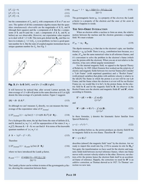
unique quantum number for S z . See Fig. 3
Fig. 3. J = L+S (left), and J + (1+ε)S (right).
It will however be noticed that, after several Larmor periods, the
time-average of (1+ε)S will point in the same direction as J. Let §Q§
denote the time-average of a periodic motion. Figure 3 suggests
§S§ = (S · J) J/J 2 . (113)
So although we can’t measure S z directly, we can measure the time
average of the expectation value of H’ Zeeman :
§ ^H’ Zeeman & § = −(q/2m) [1 + (1+ε)(S ·J)/J 2 ] (J · B o ) . (114)
For a hydrogen-like atom, the |ψ& that forms the state of definite J, L,
and S, denoted |n j m j s&, will be superposition of the states | m s
m s &[7]. Because L = J − S, we can find J · S in terms of the knowable
quantum numbers of |n j m j s&:
J · S = ½(J 2 − L 2 + S 2 ) . (115)
Therefore
§ ^H’ Zeeman & § = g Landé (q/2m) ^J · B o & (116)
where we have introduced the Landé g-factor,
g Landé = 1 + (1+ε)[j(j+1) − (+1) + ¾] . (117)
2j(j+1)
The Landé g-factor can be written in terms of the gyromagnetic g-factor,
showing the connection between them:
g Landé = 1 + (g o − 1)[j(j+1) − (+1) + ¾] . (118)
2j(j+1)
The gyromagnetic factor g o is a property of the electron; the Landé
g-factor is a property of the electron and the state of the atom in
which it happens to reside.
THE SPIN-ORBIT INTERACTION
When an electron orbits a nucleus to form an atom, the relative
motion between the nucleus and the electron generates a magnetic
field. We must evaluate
H’ int = −m 2 · B int (119)
The dipole moment m 2 is that due to the electron’s spin, our familiar
friend m = g o (q/2m)S. There is no m L contribution here because, as a
scalar, H’ int has the same numerical value in all reference frames, and
it’s convenient to solve the problem in the electron’s frame (which
sees the proton orbit the electron). When you are at rest relative to the
electron, it has zero orbital angular momentum!
For the internal magnetic field, we appeal to the Special Theory
of Relativity. In 1905 Albert Einstein first worked out the relativity of
electric and magnetic fields between two inertial frames.[8] Consider
a “Lab Frame” (with unprimed quantities) and a “Rocket Frame”
(with primed variables) that glides with uniform velocity v relative to
the lab.[9] The frame in which the proton is at rest will be our Lab
Frame, and the frame where the electron is at rest will be our Rocket
Frame (or, we would like it to be!). In the proton frame, let the electric
field be E and let the magnetic field be B. An observer in the
Rocket Frame sees the electric and magnetic fields E’ and B’, where
according to Einstein,
and
E’ = γ(E + v×B) − γ 2 v(v·E) (120)
_______ _______
(γ+1)c 2
B’ = γ(B − v×E/c 2 ) − γ 2 v(v·B) . (121)
______ _______
(γ+1)c 2
In these formulas, γ denotes the kinematic factor familiar from
Special Relativity:
γ = (1 − v 2 /c 2 ) −½ . (122)
In the problem before us, the proton produces an electric field E but
no magnetic field in its own frame. Therefore B = 0 and
B’ = −γ v×E/c 2 (123)
describes (almost!) the magnetic field “seen” by the electron. Are we
ready to import this result into Eq. (119) to assume its role for B int ?
Not quite; the transformation we have used for the electric and magnetic
fields hold between inertial reference frames, where one frame
moves with constant velocity relative to the other. However, our electron
orbits the proton; hence the electron finds itself in an accelerated
frame of reference. Happily, the correction we need for B’ is an
additive correction, as Thomas showed us in 1927. To Thomas’ correction
we now turn.
PAGE 10