Elegant Connections in Physics: Quantized Angular Momentum, 'g ...
Elegant Connections in Physics: Quantized Angular Momentum, 'g ...
Elegant Connections in Physics: Quantized Angular Momentum, 'g ...

Create successful ePaper yourself
Turn your PDF publications into a flip-book with our unique Google optimized e-Paper software.
<strong>Elegant</strong> <strong>Connections</strong> <strong>in</strong> <strong>Physics</strong>: <strong>Quantized</strong> <strong>Angular</strong><br />
<strong>Momentum</strong>, ‘g-factors,’ Precessions, and Exchange<br />
Symmetry<br />
— by Dwight E. Neuenschwander<br />
In our study of the vector algebra used <strong>in</strong> general physics, we<br />
learned that the cross product of a vector with itself vanishes: A×A =<br />
0. However, quantum mechanics shows an exception to this “obvious”<br />
identity, <strong>in</strong> the peculiar case of angular momentum L,<br />
L×L = i\ L, (1)<br />
which vanishes only <strong>in</strong> the classical limit \ O 0. This weird property<br />
of quantized angular momentum is <strong>in</strong>herited from a peculiar <strong>in</strong>terpretation<br />
of l<strong>in</strong>ear momentum, which itself emerges as an immediate<br />
consequence of the wave-particle duality postulates of deBroglie,<br />
Planck, and E<strong>in</strong>ste<strong>in</strong>.<br />
The bizarre cross product of Eq. (1) succ<strong>in</strong>ctly summarizes the<br />
commutation relations that exist among L x , L y , and L z , <strong>in</strong> particular,<br />
[L α , L β ] = i\ ε αβγ L γ (2)<br />
(α, β, and γ stand for x, y, and z and ε αβγ = +1(−1) if αβγ is an even<br />
(odd) permutation of xyz and ε αβγ = 0 if any two <strong>in</strong>dices are equal).<br />
We also learned <strong>in</strong> our quantum courses that every component commutes<br />
with the square of the angular momentum vector itself:<br />
[L 2 , L α ] = 0. (3)<br />
Where do these commutation relations come from? They come<br />
from merg<strong>in</strong>g the familiar def<strong>in</strong>ition of angular momentum with the<br />
quantum <strong>in</strong>terpretation of l<strong>in</strong>ear momentum! First, we recall the<br />
familiar def<strong>in</strong>ition of L: if a particle has l<strong>in</strong>ear momentum p, and is<br />
located by the position vector r relative to some po<strong>in</strong>t O, then that<br />
particle’s angular momentum about O is def<strong>in</strong>ed by<br />
L ≡ r×p. (4)<br />
Meanwhile, accord<strong>in</strong>g to quantum mechanics, whenever a particle’s<br />
momentum p appears <strong>in</strong> a formula we can replace p with (\/i)∇.<br />
Where does this weird assertion come from? It goes back to the<br />
deBroglie and Planck-E<strong>in</strong>ste<strong>in</strong> hypotheses, the basic postulates of<br />
quantum mechanics: Correspond<strong>in</strong>g to a free particle of momentum<br />
p and energy E, there exists a harmonic wave of wavenumber k and<br />
angular frequency ω, where, numerically, the particle properties are<br />
related to the wave properties by Planck’s constant \:<br />
E = \ω (5)<br />
and<br />
p = \k. (6)<br />
Any harmonic ψ mov<strong>in</strong>g along the x-axis always conta<strong>in</strong>s the factor<br />
ψ ~ exp[i(kx ± ωt)] (7)<br />
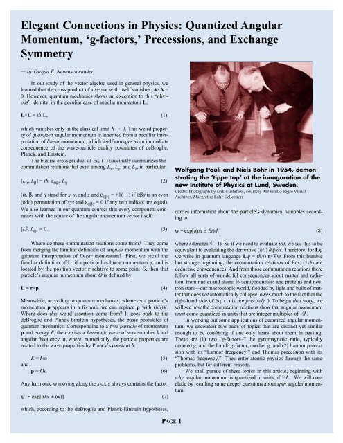
Wolfgang Pauli and Niels Bohr <strong>in</strong> 1954, demonstrat<strong>in</strong>g<br />
the ‘tippe top’ at the <strong>in</strong>auguration of the<br />
new Institute of <strong>Physics</strong> at Lund, Sweden.<br />
Credit: Photograph by Erik Gustafson, courtesy AIP Emilio Segrè Visual<br />
Archives, Margrethe Bohr Collection<br />
carries <strong>in</strong>formation about the particle’s dynamical variables accord<strong>in</strong>g<br />
to<br />
ψ ~ exp[i(px ± Et)/\] (8)<br />
where i denotes √(−1). So if we need to evaluate pψ, we see this to be<br />
equivalent to evaluat<strong>in</strong>g the derivative (\/i) ∂ψ/∂x. Therefore, for Lψ<br />
we write <strong>in</strong> quantum language Lψ = (\/i) r×∇ψ. From this humble<br />
but strange beg<strong>in</strong>n<strong>in</strong>g, the commutation relations of Eqs. (1-3) are<br />
deductive consequences. And from those commutation relations there<br />
follow all sorts of wonderful consequences about matter and radiation,<br />
from nuclei and atoms to semiconductors and prote<strong>in</strong>s and neutron<br />
stars—our macroscopic world, flooded by light and built of matter<br />
that does not automatically collapse, owes much to the fact that the<br />
right-hand side of Eq. (1) is not precisely 0. To beg<strong>in</strong> that story, we<br />
will see how the commutation relations show that angular momentum<br />
must come quantized <strong>in</strong> units that are <strong>in</strong>teger multiples of ½\.<br />
In work<strong>in</strong>g out some applications of quantized angular momentum,<br />
we encounter two pairs of topics that are dist<strong>in</strong>ct yet similar<br />
enough to be confus<strong>in</strong>g if one only hears about them <strong>in</strong> pass<strong>in</strong>g.<br />
These are (1) two “g-factors–” the gyromagnetic ratio, typically<br />
denoted g; and the Landé g-factor, another g; and (2) Larmor precession<br />
with its “Larmor frequency,” and Thomas precession with its<br />
“Thomas frequency.” They enter atomic physics through the same<br />
problems, but for different reasons.<br />
We shall pursue of these topics <strong>in</strong> this article, beg<strong>in</strong>n<strong>in</strong>g with<br />
why angular momentum is quantized <strong>in</strong> units of ½\. We will conclude<br />
by recall<strong>in</strong>g some deeper questions about sp<strong>in</strong> angular momentum.<br />
which, accord<strong>in</strong>g to the deBroglie and Planck-E<strong>in</strong>ste<strong>in</strong> hypotheses,<br />
PAGE 1
WHY ANGULAR MOMENTUM IS QUANTIZED IN UNITS<br />
OF ½\<br />
Even though a vector <strong>in</strong> physical space is supposed to be<br />
described by three numbers, the commutation relations for L mean<br />
that we can simultaneously measure for this vector, at most, only two<br />
numbers. They are its magnitude |L| (through L 2 ) and one (but only<br />
one) component, which for def<strong>in</strong>iteness we will designate L z . A system<br />
that carries quantized angular momentum will be described by<br />
some state vector |ψ& that is an eigenvector of both L 2 and L z . Let<br />
their respective eigenvalues be λ and µ, so that<br />
L 2 |ψ& = λ |ψ& (9)<br />
and<br />
L z |ψ& = µ |ψ& . (10)<br />
For our first job we must f<strong>in</strong>d λ and µ. Because Planck’s constant \<br />
carries the dimensions of angular momentum, dimensional analysis<br />
requires that λ must be proportional to \ 2 and µ must be proportional<br />
to \.<br />
For the purpose of determ<strong>in</strong><strong>in</strong>g λ and µ (and we must admire the<br />
cleverness of whoever first came up with this) we def<strong>in</strong>e the quantities<br />
L ± = L x ± iL y . (11)<br />
It’s the components of angular momentum that we can’t observe that<br />
hold the key to f<strong>in</strong>d<strong>in</strong>g out what we can observe! From the commutation<br />
relation of Eq. (3) we have at once<br />
[L 2 , L ± ] = 0 (12)<br />
which means that the state<br />
L ± |ψ& ≡ |ψ ± & (13)<br />
is also, like |ψ&, an eigenstate of L 2 , but with some as-yet-unknown<br />
eigenvalue λ’,<br />
L 2 |ψ ± & = λ’ |ψ ± &. (14)<br />
OK then, because L 2 and L ± commute, λ = λ’, as can be easily<br />
demonstrated:<br />
L 2 |ψ ± &<br />
= L 2 (L x ± iL y )|ψ&<br />
= (L x ± iL y )L 2 |ψ&<br />
= (L x ± iL y )λ |ψ&<br />
= λ|ψ ± &. (15)<br />
And from the commutation relation of Eq. (2) it follows that<br />
[L z , L ± ] = ± \L ± . (16)<br />
Consider then the effect of operat<strong>in</strong>g on |ψ ± & with L z :<br />
This means that the operators L + and L − create a set of “rungs” <strong>in</strong> a<br />
“ladder” of angular momentum states, where each differs from its<br />
neighbor by one quantum \. Evidently we can write the eigenvalue<br />
equation<br />
L z |ψ ± & = µ’ |ψ ± & (18)<br />
where µ’ = µ ± \. What a beautiful result!—L + raises and L − lowers<br />
the L z eigenvalue of |ψ& by one quantum, \.<br />
Because the component of a vector cannot exceed <strong>in</strong> magnitude the<br />
vector itself, so that <strong>in</strong> our case |L z | ≤ |L|, there must exist a state with<br />
a maximum L z , call it |ψ top &, such that<br />
L + |ψ top & = 0. (19)<br />
Let |ψ top & have L z eigenvalue µ top , which says<br />
L z |ψ top & = µ top |ψ top &. (20)<br />
From dimensional analysis, it must happen that<br />
µ top = \ (21)<br />
for some dimensionless number . So now we must f<strong>in</strong>d . Because<br />
λ depends only on L 2 and not upon L z , we may write for |ψ top &<br />
L 2 |ψ top & = λ |ψ top & . (22)<br />
Let’s write the left-hand side of this as<br />
L 2 = L x<br />
2 + L y<br />
2 + L z<br />
2<br />
= L ± L \L z + L z<br />
2. (23)<br />
Us<strong>in</strong>g the lower sign from Eq. (23), Eq. (22) becomes<br />
(L − L + + \L z + L z 2 )|ψ top & = λ |ψ top & (24)<br />
Each term on the left side we know how to evaluate, so that<br />
(0 + \ 2 + \ 2 2 ) |ψ top & = λ |ψ top & (25)<br />
and thus<br />
λ = \ 2 ( + 1). (26)<br />
Likewise, there must exist a bottom “rung” |ψ bottom & with L z eigenvalue<br />
\ ’ such that<br />
L − |ψ bottom & = 0 (27)<br />
for some dimensionless number ’. S<strong>in</strong>ce |ψ bottom & will have the<br />
same eigenvalue of L 2 as all the other angular momentum states on<br />
the “ladder,” we have<br />
L 2 |ψ bottom & = λ |ψ bottom & . (28)<br />
L z |ψ ± &<br />
= L z L ± |ψ&<br />
= (L ± L z ± \L ± ) |ψ&<br />
= (µ ± \) |ψ ± &. (17)<br />
PAGE 2<br />
So that we can make use of Eq. (27), employ the upper sign from Eq.<br />
(23) <strong>in</strong> Eq. (28),<br />
(L + L − − \L z + L z<br />
2)|ψ bottom & = λ |ψ bottom & (29)
which gives on the left-hand side<br />
\ 2 ’ (’ − 1) |ψ bottom & = λ |ψ bottom & . (30)<br />
Because it’s the same λ for |ψ top & and |ψ bottom &, it follows that<br />
\ 2 ’ (’ − 1) = \ 2 ( + 1) (31)<br />
which requires either<br />
or<br />
’ = +1 (32)<br />
’ = − . (33)<br />
The first alternative must be elim<strong>in</strong>ated physically because the lowest<br />
rung of the angular momentum state ladder cannot have a larger<br />
value of L z than the highest one! This leaves ’ = −: the bottom<br />
rung of the ladder is symmetric with the top rung.<br />
Let’s sum up what we have so far:<br />
L 2 |ψ& = \ 2 ( + 1) |ψ , (34)<br />
L z |ψ top & = \ |ψ top & , (35)<br />
L z |ψ bottom & = −\ |ψ bottom &, (36)<br />
where<br />
L z |ψ ± = (µ ± \) |ψ ± & , (37)<br />
So it seems that a particle that has angular momentum L will have<br />
quantized z-components with labels from + to −, separated by <strong>in</strong>teger<br />
steps. Def<strong>in</strong>e<br />
m = , − 1, ..., −. (38)<br />
This means that must, itself, be either an <strong>in</strong>teger or a half-<strong>in</strong>teger.<br />
Were it not, then we could not have ’ = −. For <strong>in</strong>stance, one might<br />
imag<strong>in</strong>e that, say, = 3.1, and count backwards by <strong>in</strong>teger steps, then<br />
we would encounter the sequence<br />
3.1<br />
2.1<br />
1.1<br />
0.1<br />
−0.9<br />
−1.9,<br />
−2.9<br />
−3.9...<br />
which skips over −3.1. If is an <strong>in</strong>teger or half-<strong>in</strong>teger then there are<br />
2+1 “rungs” <strong>in</strong> the “ladder” of z-component states. Let N denote the<br />
number of steps that will take us from the − state to the + state.<br />
S<strong>in</strong>ce the number of steps is one less than the number of rungs, we<br />
can say that<br />
N = 2 where N = 0,1,2,3,... (39)<br />
Therefore, may assume these possible values:<br />
= ½N = 0, ½, 1, 3/2, 2, 5/2,... (40)<br />
We have demonstrated that when a system has angular momentum L,<br />
and that system is subject to the rules of quantum mechanics, its<br />
angular momentum must be described by a quantum state with eigenvalues<br />
and m , so we denote the state as<br />
|ψ& = |, m & (41)<br />
The angular momentum has magnitude |L| where<br />
L 2 |, m & = \ 2 (+1) |, m & (42)<br />
with = 0,1,2,.... The orientation of the L vector relative to the z-axis<br />
can be <strong>in</strong> one of the directions given by<br />
L z |, m & = \ m |, m & (43)<br />
where m = , −1, ..., −. It will be noticed that the number of states<br />
of different m , for each , is 2+1, the “multiplicity” of states hav<strong>in</strong>g<br />
the same .<br />
Our knowledge of the direction of L is quite limited. Accord<strong>in</strong>g<br />
to classical mechanics, we can know the magnitude and all three<br />
components of L simultaneously, to as many decimal places (<strong>in</strong> pr<strong>in</strong>ciple)<br />
as we wish. But for quantized angular momentum, we can<br />
know, <strong>in</strong> pr<strong>in</strong>ciple, the magnitude of L but only one component of it<br />
(which we call the z-component). We have no clue about the x and y<br />
components of L, so all we can say about the angular momentum vector<br />
is that it lies somewhere on the cone whose axis is the z-axis and<br />
the cone’s surface makes the angle from the z-axis given by θ, which<br />
has a well-def<strong>in</strong>ed value when the particle is <strong>in</strong> a pure state |, m &:<br />
cosθ = ^ L z &/ =^ L 2 &<br />
= m / =( 2 + ) (44)<br />
Because for a given value of the azimuthal quantum number m <br />
takes on only 2+1 values, cosθ has only 2+1 possible values. This<br />
is sometimes mislead<strong>in</strong>gly called “space quantization;” I say “mislead<strong>in</strong>g”<br />
because its angular momentum, not space, that gets quantized.<br />
(Space might be quantized at the Planck scale 10 −33 cm, but<br />
that's another story entirely!)<br />
It’s <strong>in</strong>terest<strong>in</strong>g to compare the circumstances of the quantization<br />
of angular momentum to those necessary for the quantization of energy.<br />
In the quantum world, a particle’s energies are quantized only if<br />
the particle moves <strong>in</strong> some restricted region of space, so the<br />
deBroglie wave functions become stand<strong>in</strong>g waves of discrete frequencies.<br />
But when the particle is free, then its energy will be a cont<strong>in</strong>uous<br />
variable; the deBroglie waves are conf<strong>in</strong>ed with<strong>in</strong> no boundaries<br />
and may have any frequency whatsoever. But whether the particle<br />
is free or conf<strong>in</strong>ed makes no difference to angular momentum: It’s<br />
values of L 2 and L z are necessarily quantized, and its values of L x and<br />
L y are not measurable. This occurs because the deeper relation p =<br />
(\/i)∇ does not depend on boundary conditions.<br />
REPRESENTATIONS OF ANGULAR MOMENTUM<br />
We recall that the angular momentum of a system of particles (<strong>in</strong><br />
both the Newtonian or quantum paradigms) can be partitioned <strong>in</strong>to<br />
the “orbital angular momentum” of the center of mass relative to<br />
some orig<strong>in</strong>, plus the “sp<strong>in</strong> angular momentum” about the center of<br />
mass.[1] Henceforth <strong>in</strong> this article, I will let L denote the orbital<br />
angular momentum, S the sp<strong>in</strong> angular momentum, and J their sum:<br />
PAGE 3
J = L + S. (45)<br />
For a Newtonian example, the Earth forms an extended body, orbit<strong>in</strong>g<br />
the Sun while sp<strong>in</strong>n<strong>in</strong>g on its axis. The Earth’s total angular<br />
momentum J can be partitioned <strong>in</strong>to the angular momentum L of the<br />
Earth’s center of mass about the Sun, plus its sp<strong>in</strong> angular momentum<br />
about the center of mass. L is the Earth’s angular momentum as if it<br />
were a s<strong>in</strong>gle particle with no size or shape—a po<strong>in</strong>t mass. The details<br />
of its size and shape are carried by the sp<strong>in</strong> angular momentum S as<br />
the Earth sp<strong>in</strong>s on its axis.<br />
Such a partition—at least a result analogous to it—also occurs<br />
for the electron <strong>in</strong> an atom. The orbital angular momentum states that<br />
go with L will be denoted |, m &, and the sp<strong>in</strong> angular momentum<br />
states that go with S will be denoted |s, m s &. Whatever the values of<br />
(<strong>in</strong>teger or half-odd <strong>in</strong>teger), we have seen how the values of m differ<br />
by <strong>in</strong>teger steps, rang<strong>in</strong>g from − to +; and likewise, whatever<br />
the values of s (<strong>in</strong>teger or half-odd <strong>in</strong>teger), the values of m s also differ<br />
by <strong>in</strong>teger steps and range from −s to +s. What are these values,<br />
and what do the states |, m & and |s, m s & look like explicitly? By that<br />
question I mean, what k<strong>in</strong>ds of <strong>in</strong>formation do they conta<strong>in</strong>, and how<br />
do we encode that <strong>in</strong>formation? (We will worry about the J states<br />
later.)<br />
When we neglect any details that may exist about the electron’s<br />
size and shape (if it has a size and shape) and ignore its sp<strong>in</strong> for the<br />
moment (as one does when deriv<strong>in</strong>g Kepler’s laws for po<strong>in</strong>t-mass<br />
planets orbit<strong>in</strong>g the Sun), we are then consider<strong>in</strong>g orbital angular<br />
momentum only. Consider the situation where the electron moves <strong>in</strong><br />
the potential of a central force, that acts only <strong>in</strong> the radial dimension,<br />
and thus exhibits spherical symmetry about the orig<strong>in</strong>. Central forces<br />
exert no torque and thus conserve orbital angular momentum. The<br />
particle’s k<strong>in</strong>etic plus potential energy sums to the total,<br />
p 2 /2m + U = E (46)<br />
which gets echoed <strong>in</strong> quantum mechanics <strong>in</strong> the time-<strong>in</strong>dependent<br />
Schröd<strong>in</strong>ger equation for the energy eigenvalues E,<br />
−(\ 2 /2m)∇ 2 ψ + U(r)ψ = Eψ . (47)<br />
Keep <strong>in</strong> m<strong>in</strong>d that the orbital angular momentum L is already<br />
built <strong>in</strong>to Eqs. (46) and (47). How does l<strong>in</strong>ear momentum p get<br />
turned <strong>in</strong>to angular momentum L? It’s through the k<strong>in</strong>etic energy,<br />
because both p and L depend on the orbit<strong>in</strong>g particle hav<strong>in</strong>g a velocity.<br />
First, note that because a central force exerts zero torque on the<br />
orbiter, L = constant <strong>in</strong> both magnitude and direction. So we can take<br />
the direction of L to po<strong>in</strong>t along the z-axis, which means the particle<br />
orbits <strong>in</strong> the equatorial plane. Second, the l<strong>in</strong>ear momentum p has<br />
radial component mdr/dt and angular component mrdφ/dt. This<br />
means that |L| = |r×p| = m r 2 dφ/dt. F<strong>in</strong>ally, the k<strong>in</strong>etic energy p 2 /2m<br />
or ½mv 2 may be written <strong>in</strong> terms of angular momentum:<br />
½m v·v = ½m(dr/dt) 2 + ½mr 2 (dφ/dt) 2<br />
= ½m(dr/dt) 2 + ½L 2 /mr 2 . (48)<br />
With a central potential energy (that does not depend on latitude,<br />
longitude, or time), <strong>in</strong> the spherical coord<strong>in</strong>ates (r, θ, φ) of Fig. 1, the<br />
Schröd<strong>in</strong>ger equation separates.<br />
Fig. 1. Spherical coord<strong>in</strong>ates.<br />
To carry this out, one factors the wave function <strong>in</strong>to radial and angular<br />
parts: ψ(r, θ, φ) = R(r)Y(θ, φ). The Schröd<strong>in</strong>ger equation neatly<br />
separates <strong>in</strong>to one equation that has only r-dependence, and another<br />
equation hav<strong>in</strong>g only the θ and φ dependence of latitude and longitude.<br />
The separation constants that enable the angular and radial parts<br />
to uncouple turn out to be none other than our now-familiar friend<br />
(but here obta<strong>in</strong>ed from another approach!):<br />
( +1) for = 0,1,2,3,...<br />
The angular equation separates a second time <strong>in</strong>to an equation for θ<br />
and another equation for φ. The separation constant that enables the θ<br />
dependence to separate from φ is another of our friends,<br />
m = , −1,..., −.<br />
So <strong>in</strong> the case of a particle mov<strong>in</strong>g <strong>in</strong> any central potential, the orbital<br />
angular momentum states carry <strong>in</strong>tegral quantum numbers and their<br />
correspond<strong>in</strong>g <strong>in</strong>tegers m .<br />
What do the correspond<strong>in</strong>g orbital angular momentum states<br />
|, m & look like explicitly? What <strong>in</strong>formation do they conta<strong>in</strong>, besides<br />
the numerical values of and m ? When you solve the partial differential<br />
equations for the latitude and longitude variables <strong>in</strong> the central<br />
potential problem (where the angular equation is <strong>in</strong>dependent of the<br />
potential), the solutions are the celebrated spherical harmonics,<br />
denoted Y m (θ,φ). They are comb<strong>in</strong>ations of s<strong>in</strong>es and cos<strong>in</strong>es of θ<br />
and φ. The spherical harmonics, as their name suggests, form an<br />
orthonormal basis for any function of latitude and longitude on a<br />
spherical surface. The spherical harmonics arise not only <strong>in</strong> quantum<br />
central force problems, but they appear ubiquitously <strong>in</strong> otherwise<br />
unrelated topics too, that take for their subject matter functions<br />
def<strong>in</strong>ed on spherical surfaces. Applications range from electrostatics<br />
to heliosiesmology. The spherical harmonics describe “stand<strong>in</strong>g<br />
waves” that may exist on a spherical surface, <strong>in</strong> terms of which any<br />
function of latitude and longitude can be expressed by their superposition.<br />
Students of quantum theory (and general chemistry, which is<br />
applied physics) will recognize <strong>in</strong> the shapes of the hydrogen atom<br />
orbitals the first few spherical harmonics: on a sphere of any specific<br />
radius centered on the nucleus, the spherical harmonics for a given <br />
and m describes how the probability density varies with latitude and<br />
PAGE 4
longitude when the system exists <strong>in</strong> that pure “stand<strong>in</strong>g wave” mode.<br />
Of course, at any moment the actual wave function for the electron <strong>in</strong><br />
the hydrogen atom will be a superposition of the solutions we have<br />
just described, just as the actual wave on the cello str<strong>in</strong>g is some l<strong>in</strong>ear<br />
comb<strong>in</strong>ation of its harmonic series of possible stand<strong>in</strong>g waves.<br />
When the central potential <strong>in</strong> the Schröd<strong>in</strong>ger equation happens<br />
to be the Coulomb <strong>in</strong>teraction between a po<strong>in</strong>t nucleus and a s<strong>in</strong>gle<br />
po<strong>in</strong>t electron, the radial equation can be solved exactly giv<strong>in</strong>g a set<br />
of functions R(r) that depends on and another quantum number n<br />
<strong>in</strong>troduced below. Each such function consists of a Laguerre polynomial,<br />
multiplied by an exponentially damped radial factor. One<br />
derives here a third quantum number, denoted n, that may take on the<br />
values n = 1,2,3,.... The electron’s energy levels <strong>in</strong> the Coulomb-only<strong>in</strong>teraction<br />
of a s<strong>in</strong>gle electron <strong>in</strong> the hydrogen atoms are given by<br />
E n = −a 2 mc 2 (1/n 2 )<br />
= −13.6eV/n 2 , (49)<br />
where<br />
a = ke 2 /\c ≈ 1/137 (50)<br />
denotes the “f<strong>in</strong>e structure constant,” a dimensionless comb<strong>in</strong>ation of<br />
the fundamental constants from electrodynamics (the Coulomb constant<br />
k and the fundamental charge e), quantum theory (Planck's constant),<br />
and special relativity (the speed of light). The f<strong>in</strong>e structure<br />
constant sets the scale of the photon-charge <strong>in</strong>teraction <strong>in</strong> quantum<br />
electrodynamics.<br />
Back to the hydrogen atom: when work<strong>in</strong>g out the solution of<br />
this problem, it’s useful to organize the states by start<strong>in</strong>g with n,<br />
which takes on the possible values 1,2,3,.... If you know n, then the<br />
values of will be 0,1,2,... up to n−1, and when you know then the<br />
values of m range <strong>in</strong> <strong>in</strong>teger steps from + to −. A moment’s reflection<br />
shows that for each n there are n 2 states all with the same energy<br />
<strong>in</strong> the Coulomb-only <strong>in</strong>teraction model of the hydrogen atom.<br />
But of course, there are more <strong>in</strong>teractions between the orbit<strong>in</strong>g<br />
electron and the proton than are captured by the electrostatic<br />
Coulomb <strong>in</strong>teraction! The relative motion between the electron and<br />
proton means generates an <strong>in</strong>ternal magnetic field with<strong>in</strong> the atom.<br />
This <strong>in</strong>teraction reveals itself through the electron’s sp<strong>in</strong> angular<br />
momentum.<br />
The electron energy levels show up through their differences, <strong>in</strong><br />
the energy spectrum of the photons that make transitions between<br />
those levels. However, there’s a subtle f<strong>in</strong>e structure: each (n, , m )<br />
energy state seems to be doubled <strong>in</strong>to a pair of states! We have not<br />
yet <strong>in</strong>cluded the possibility of sp<strong>in</strong> angular momentum for the electron,<br />
so if we now assume this doubl<strong>in</strong>g to be somehow <strong>in</strong>volved with<br />
the electron’s sp<strong>in</strong>, it appears that the electron’s sp<strong>in</strong> angular momentum<br />
has a multiplicity of 2, that is,<br />
2s + 1 = 2<br />
so that<br />
s = ½<br />
and therefore<br />
m s = ±½.<br />
beam of free electrons and pass<strong>in</strong>g them through a slit followed by a<br />
magnetic field: the beam of electrons splits <strong>in</strong>to two beams. When<br />
one tries to further split the separated beams aga<strong>in</strong> with magnets oriented<br />
the same way as the first magnet, no further splitt<strong>in</strong>g of the<br />
beams occur. The first magnet separates the electrons accord<strong>in</strong>g to<br />
their two possible sp<strong>in</strong> polarization states.<br />
These two states, sp<strong>in</strong> up and sp<strong>in</strong> down, can serve as the basis<br />
states for a two-state system. Sp<strong>in</strong> up and sp<strong>in</strong> down “basis vectors”<br />
can be represented by a pair of two-component matrices:<br />
|s, m s & = |½, + ½¬ = ⎡1⎤ ≡ χ +<br />
⎣0⎦<br />
and<br />
|s, m s & = |½, − ½¬ = ⎡0⎤ ≡ χ −<br />
⎣1⎦<br />
(51a)<br />
(51b)<br />
Any possible sp<strong>in</strong> state may be written as a superposition of these<br />
basis states:<br />
χ ≡ ⎡u⎤ = u ⎡1⎤ + v ⎡0⎤ = u χ + + v χ − (52)<br />
⎣v⎦ ⎣0⎦ ⎣1⎦<br />
where |u| 2 = probability that the electron will be found to have sp<strong>in</strong><br />
up, and |v| 2 = probability that it will be found to have sp<strong>in</strong> down,<br />
when the sp<strong>in</strong> is measured. In the case of the electron,<br />
S 2 χ ± = \ 2 s(s+1) χ ± = ¾\ 2 χ (53)<br />
and<br />
S z χ ± = ±½\ χ ± (54)<br />
Once we write the sp<strong>in</strong> state as a two-entry column matrix, then<br />
any manipulation of the sp<strong>in</strong>, any way to query or modify the <strong>in</strong>formation<br />
conta<strong>in</strong>ed <strong>in</strong> the sp<strong>in</strong> matrices, must be represented with 2×2<br />
matrices. Let’s construct a set of such matrices <strong>in</strong> terms of which the<br />
sp<strong>in</strong> <strong>in</strong>formation can be manipulated.<br />
From Eq. (53) we can see that a matrix representation for S 2 is<br />
S 2 = ¾\ 2 ⎡1 0⎤ (55)<br />
⎣0 1⎦ .<br />
Eq. (54) suggests the matrix representation for S z as<br />
S z = ½\ ⎡1 0⎤ (56)<br />
⎣0−1⎦ .<br />
We also recall the rungs of our “ladder” of states, where for the top<br />
and bottom rungs (the sp<strong>in</strong>-½ ladder has only two rungs!),<br />
S + χ + = 0 (57)<br />
and<br />
S − χ − = 0. (58)<br />
On such considerations, sp<strong>in</strong>-½ for the electron was proposed by<br />
Uhlenbeck and Goudsmit <strong>in</strong> 1926. Their hypothesis means that S z has<br />
only two possible orientations, which we refer to casually as “sp<strong>in</strong><br />
up” and “sp<strong>in</strong> down,” a sp<strong>in</strong> polarization.<br />
The magnetic field <strong>in</strong>ternal to the atom only reveals the sp<strong>in</strong>; it<br />
does not cause sp<strong>in</strong>. The sp<strong>in</strong> of the electron is a property of the electron<br />
itself, not merely of its habitat. This can be shown by tak<strong>in</strong>g a<br />
PAGE 5<br />
In terms of matrices these relations will be satisfied by<br />
S + = \ ⎡0 1⎤ (59)<br />
⎣0 0⎦<br />
and<br />
S − = \ ⎡0 0⎤ (60)<br />
⎣1 0⎦
But from the def<strong>in</strong>ition of S ± = S x + iS y it follows that<br />
S x = ½(S + + S − ) (61)<br />
and<br />
S y = −½ i (S + − S − ) (62)<br />
Therefore<br />
and<br />
S x = ½\ ⎡0 1⎤ (63)<br />
⎣1 0⎦<br />
S y = ½\ ⎡0 −i⎤ (64)<br />
⎣i 0⎦<br />
The sp<strong>in</strong> vector S for a sp<strong>in</strong>-½ can now be represented as a “vector of<br />
matrices,”<br />
S = S x i + S y j + S z k = ½\ σ (65)<br />
where σ denotes the celebrated “Pauli sp<strong>in</strong> matrices,”<br />
σ x = ⎡0 1⎤ σ y = ⎡0 −i⎤ σ z = ⎡1 0⎤ (66)<br />
⎣1 0⎦ ⎣i 0⎦ ⎣0 −1⎦ .<br />
The mental picture of the electron as a wee little top is quite suggestive,<br />
of course; but it’s mislead<strong>in</strong>g if taken literally. Although the electron’s<br />
sp<strong>in</strong> behaves algebraically like any other quantized angular<br />
momentum, and by that standard is def<strong>in</strong>itely an angular momentum,<br />
it can’t be as simple as the familiar mechanical motion of a t<strong>in</strong>y sp<strong>in</strong>n<strong>in</strong>g<br />
top. Here’s why: it’s a useful exercise to calculate the speed of a<br />
po<strong>in</strong>t on a spherical electron’s equator, if its radius is determ<strong>in</strong>ed by<br />
sett<strong>in</strong>g its electrostatic energy equal to mc 2 , and sett<strong>in</strong>g the product of<br />
its moment of <strong>in</strong>ertia and angular velocity equal to ½\. One f<strong>in</strong>ds that<br />
a po<strong>in</strong>t on the equator moves at someth<strong>in</strong>g like 300 times the speed<br />
of light![2] Clearly a mechanical model cannot be taken literally (at<br />
least, not if the mass is associated with the electric energy density).<br />
Whatever the mechanism that causes sp<strong>in</strong>, it seems to be an <strong>in</strong>tr<strong>in</strong>sic<br />
property of each species of elementary particle. Indeed, one def<strong>in</strong>ition<br />
of an elementary particle has been offered as “a state of def<strong>in</strong>ite mass<br />
and sp<strong>in</strong>.”[3] Electrons, quarks, and neutr<strong>in</strong>os are elementary particles<br />
that have s = ½; photons have s = 1, gravitons (when they are<br />
detected) will have s = 2; the Higgs particles (or whatever <strong>in</strong> Nature<br />
plays the role of the conjectured Higgs particles) have s = 0.<br />
Composite objects such as protons and neutrons (bound states of<br />
quarks) or the helium-3 nucleus have odd-half-<strong>in</strong>teger \; composites<br />
such as pions or the helium-4 nucleus have <strong>in</strong>teger s. Particles with<br />
<strong>in</strong>teger s are called “bosons,” and particles with odd-half-<strong>in</strong>teger s are<br />
called “fermions.” When one encounters a system of two or more<br />
identical particles, it matters mightily whether they are bosons or<br />
fermions. More about that later.<br />
If the elementary particle (or composite) carries some distribution<br />
of electric charge (even if it’s electrically neutral overall, like the<br />
neutron), then from the def<strong>in</strong>ition of the angular momentum of an<br />
extended body, and from the def<strong>in</strong>ition of a current distribution’s<br />
magnetic dipole moment, it follows that there should be, <strong>in</strong> general, a<br />
connection between sp<strong>in</strong> and magnetic dipole moment. To that topic<br />
we turn next.<br />
THE GYROMAGNETIC RATIO<br />
Deep <strong>in</strong>elastic collisions show that the size (if such exists) of an<br />
electron must be smaller than a scale on the order of 10 −18 cm, about<br />
a hundred thousand times smaller than the proton. On the other hand,<br />
if the electron really is a genu<strong>in</strong>e particle—a po<strong>in</strong>t mass—how can a<br />
po<strong>in</strong>t be endowed with a dipole moment (magnetic or otherwise)?<br />
Leav<strong>in</strong>g those fasc<strong>in</strong>at<strong>in</strong>g questions aside, as a mechanical concept<br />
the sp<strong>in</strong> angular momentum would be a superposition of the sum of<br />
all the angular momenta of its parts distributed about the center of<br />
mass:<br />
S = * r×v dm<br />
= * r×v ρ mass dV (67)<br />
where ρ mass denotes the electron’s mass density and dV a volume element<br />
(if the electron were a genu<strong>in</strong>e po<strong>in</strong>t mass, then the density<br />
would be the mass times the Dirac delta function). Similarly, because<br />
this sp<strong>in</strong>n<strong>in</strong>g mass carries electric charge, its various parts make little<br />
current loops which generates a magnetic dipole.[4] When one does<br />
the multipole expansion for the magnetic field produced by a generic<br />
electric current distribution, the dipole field dom<strong>in</strong>ates. The magnetic<br />
dipole moment µ emerges as a coefficient <strong>in</strong> the expansion:<br />
m = ½ * r×j dV<br />
= ½ * r×v ρ charge dV (68)<br />
where j denotes the current density and ρ charge the charge density. It<br />
will be noticed that, aside from the ½ (that comes from the Taylor<br />
series <strong>in</strong> the multipole expansion), the def<strong>in</strong>itions of S and µ are<br />
almost identical, the only difference be<strong>in</strong>g that one has mass density<br />
and the other has charge density. If we divide the respective densities<br />
by the total charge and total mass, then take the ratio of these specific<br />
densities, we have a dimensionless number called the “gyromagnetic<br />
g-factor,” here denoted g o :<br />
(ρ charge /q)<br />
g o [ (70)<br />
(ρ mass /m).<br />
In general, both densities may be a function of location; but if g o<br />
does not vary throughout the electron’s volume, or if we are content<br />
with the ratio of average densities, then we see that<br />
m = g o (q/2m)S. (71)<br />
g o (q/2m) is called the “gyromagnetic ratio,” (denoted γ <strong>in</strong> many<br />
works), the ratio of the electron’s attributes as a mechanical gyroscope<br />
and a magnet. Because the electron’s charge is negative, q =<br />
−e, its magnetic dipole moment po<strong>in</strong>ts opposite the sp<strong>in</strong> vector. That<br />
means, for the electron, “sp<strong>in</strong> up” has higher energy than “sp<strong>in</strong> down”<br />
<strong>in</strong> the dipole-field potential energy −m · B, of which more will be said<br />
shortly.<br />
If the electric charge were distributed exactly the same as the<br />
mass then g o would equal 1; therefore any deviation from unity suggests<br />
that the electric charge and mass are not identically distributed.<br />
The gyromagnetic ratios of the proton and neutron are about 5.586<br />
and −3.826 respectively. Such numbers provide evidence that the proton<br />
and neutron are not elementary particles, but composites, <strong>in</strong> their<br />
case are built of quarks and gluons.<br />
Uhlenbeck and Goudsmit <strong>in</strong>itially suggested g o = 2 for the electron,<br />
because that would fit the data available to them <strong>in</strong> 1926. For the<br />
PAGE 6
electron the Dirac equation predicts g o = 2, twice the value one would<br />
expect if the electron were a little ball that carried uniform charge<br />
density and uniform mass density with those densities distributed<br />
identically over the same volume. Evidently the distributions of mass<br />
and charge are not identical. It gets even more complicated: higherorder<br />
corrections <strong>in</strong> perturbative quantum mechanics (evaluat<strong>in</strong>g<br />
higher-order Feynman diagrams, through six and eight electron-photon<br />
vertices) show a power series <strong>in</strong> the f<strong>in</strong>e structure constant,<br />
g o = 2 + α/π + ... (72)<br />
where α denotes aga<strong>in</strong> the f<strong>in</strong>e structure constant. High-order calculations<br />
from perturbation theory, along with precision measurements<br />
of g o −2, provide sensitive tests of quantum electrodynamics (another<br />
story <strong>in</strong> its own right).[5] There’s a lot of physics (not all of it<br />
understood) even <strong>in</strong> the humble electron! However, a discussion of<br />
those topics here would take us too far afield. I mention them only to<br />
show the connections between the path we follow here, and other<br />
routes that <strong>in</strong>tersect ours <strong>in</strong> the rich conceptual space of physics.<br />
Here I want to talk about another k<strong>in</strong>d of “g-factor” and two k<strong>in</strong>ds of<br />
precession. Let’s turn first to Larmor precession.<br />
LARMOR PRECESSION<br />
This is merely the usual precession that all gyroscopes experience<br />
when acted on by a torque, but we call it “Larmor precession”<br />
when the gyroscope happens to a magnetic dipole placed <strong>in</strong> a magnetic<br />
field. Let’s review the precession of gyroscopes generically.<br />
Let a top have sp<strong>in</strong> angular momentum S and let some torque<br />
r×F act on it thanks to a lever arm r. Newton’s Second Law <strong>in</strong> its<br />
rotational form, applied to the top, says<br />
r×F = dS/dt. (73)<br />
Let the sp<strong>in</strong> axis of the top be oriented at angle θ with respect to the<br />
z-axis, and let the force be parallel or antiparallel to the z-axis. For<br />
example, <strong>in</strong> the case of gravity, F po<strong>in</strong>ts vertically down and this will<br />
produce a torque on the top’s center of mass given <strong>in</strong> magnitude by<br />
rFs<strong>in</strong>θ, and with a direction that po<strong>in</strong>ts <strong>in</strong> the direction <strong>in</strong>dicated by<br />
Fig. 2.<br />
But dφ/dt is an angular frequency ω, and thus<br />
ω = rF/S . (75)<br />
In the case of a magnetic dipole m that f<strong>in</strong>ds itself <strong>in</strong> some magnetic<br />
field B, Newton’s Second Law gives<br />
m×B = dS/dt (76)<br />
where we recall that m = g o (q/2m)S. The same analysis of the torque<br />
and the precession response to it carries through, with µB tak<strong>in</strong>g the<br />
place of rF. Now we have for the frequency of precession, <strong>in</strong> this context<br />
called the Larmor frequency,<br />
ω Larmor = g o (|q|/2m) B . (77)<br />
(We might note that, once the precession gets underway, the center of<br />
mass orbits the z-axis, which means the top now carries some orbital<br />
angular momentum <strong>in</strong> addition to the sp<strong>in</strong>. The rate of change of total<br />
angular momentum due to the torque gives “nutation” <strong>in</strong> addition to<br />
the precession, and another tangent that we don’t have space here to<br />
follow.)<br />
So, <strong>in</strong> the presence of a torque, a top <strong>in</strong> a gravitational field, or a<br />
magnetic dipole <strong>in</strong> a magnetic field, will precess. For a quantized<br />
angular momentum (whether it be L or S or J), the vector precesses<br />
on the cone described earlier. Because the angle θ of the cone cancels<br />
out of the derivation of the precession frequency, it’s the same for all<br />
θ. For a quantum sp<strong>in</strong>, we can’t track the tip of the sp<strong>in</strong> vector; all we<br />
know is that it lies somewhere on the cone.<br />
The <strong>in</strong>teraction between a magnetic dipole and an applied magnetic<br />
field produces not only a torque but also a potential energy:<br />
H’ = −m · B<br />
= −µB cosθ . (78)<br />
Recall that <strong>in</strong>formation about the electron’s sp<strong>in</strong> is carried by the twoentry<br />
row vector, or matrix χ, or “sp<strong>in</strong>or” as it’s called; <strong>in</strong> this language,<br />
any operations that manipulate the sp<strong>in</strong> state must be represented<br />
with 2×2 matrices. For example, to measure the electron’s<br />
<strong>in</strong>teraction energy with the magnetic field, we have<br />
H’ = −m · B<br />
= −g o (q/2m) S · B<br />
= −g o (q/2m) ½\ s · B (79)<br />
S<strong>in</strong>ce we def<strong>in</strong>e the direction of B to be the z-axis, as a matrix for<br />
manipulat<strong>in</strong>g the <strong>in</strong>formation <strong>in</strong> a sp<strong>in</strong> state χ we have<br />
H’ = −½\ g o (q/2m)B ⎡1 0⎤ (80)<br />
⎣0 −1⎦<br />
Fig. 2. Larmor Precession<br />
The sp<strong>in</strong> vector suffers a change dS <strong>in</strong> the same direction as the<br />
torque, and sweeps through the <strong>in</strong>crement of magnitude dS = S z dφ =<br />
S s<strong>in</strong>θ dφ. The s<strong>in</strong>θ cancels out of Newton’s Second Law, to give<br />
rF = S dφ/dt . (74)<br />
The eigenstates and eigenvalues of H’ are of course χ + with eigenvalue<br />
−½\ g o (q/2m) and χ − with eigenvalue +½\ g o (q/2m).<br />
It should be noticed that, us<strong>in</strong>g the electron’s mass and charge, if<br />
we set g o = 2 then −½\ g o (q/2m) = + e\/2m = 5.788×10 −5 eV/T, the<br />
Bohr magneton, denoted µ B <strong>in</strong> many books.<br />
Suppose an electron (or any other sp<strong>in</strong>-½ particle) f<strong>in</strong>ds itself<br />
<strong>in</strong> some generic sp<strong>in</strong> state χ, which can be expanded <strong>in</strong> the χ + and<br />
χ − basis:<br />
PAGE 7
χ = u χ + + v χ − (81)<br />
The coefficients u and v tell us, through |u| 2 and |v| 2 , the probabilities<br />
that the electron will be found to have sp<strong>in</strong> up or sp<strong>in</strong> down<br />
respectively. These probabilities are measured by count<strong>in</strong>g the fraction<br />
of particles, each <strong>in</strong> sp<strong>in</strong> state χ, that, when the sp<strong>in</strong> is measured,<br />
pops up as hav<strong>in</strong>g sp<strong>in</strong> up or sp<strong>in</strong> down. This state χ evolves<br />
<strong>in</strong> time accord<strong>in</strong>g to the Schröd<strong>in</strong>ger equation,<br />
H’ χ = (−\/i) ∂χ/∂t . (82)<br />
Split <strong>in</strong>to its two components, and temporarily lett<strong>in</strong>g ε denote<br />
−½\ g o (q/2m) for brevity, this matrix equation becomes the pair of<br />
equations<br />
εu = (−\/i) ∂u/∂t<br />
and<br />
εv = (+\/i) ∂v/∂t<br />
with solutions<br />
u(t) = u(0) e −iεt/\<br />
and<br />
v(t) = v(0) e iεt/\<br />
(83a)<br />
(83b)<br />
(84a)<br />
(84b)<br />
Because the electron when hit with a magnetic field must l<strong>in</strong>e up <strong>in</strong>to<br />
either the sp<strong>in</strong>-up state or the sp<strong>in</strong>-down state, at any time the probabilities<br />
sum to unity,<br />
1 = |u| 2 + |v| 2 (85)<br />
so that we can always write<br />
u(0) = cosδ<br />
and<br />
v(0) = s<strong>in</strong>δ<br />
(86a)<br />
(86b)<br />
for some real number δ. How does this phase angle δ for the sp<strong>in</strong> state<br />
relate to the angle θ <strong>in</strong> physical space that the sp<strong>in</strong> vector makes with<br />
the magnetic field B? For the classical dipole, θ is determ<strong>in</strong>ed from<br />
S z accord<strong>in</strong>g to<br />
S z = |S| cosθ (87)<br />
where the classical |S| can be any non-negative value from the cont<strong>in</strong>uum<br />
that we want (it does not have to be some <strong>in</strong>teger multiple of<br />
½\). Let’s calculate the expectation value of S z for quantized sp<strong>in</strong>.<br />
Here’s its physical situation: we have an ensemble of electrons, each<br />
carefully placed somehow <strong>in</strong> the state χ, the same χ for each electron<br />
<strong>in</strong> the ensemble. We hit each electron with the magnetic field and<br />
measure whether it aligns itself “sp<strong>in</strong> up” or “sp<strong>in</strong> down,” and collect<br />
statistics on the results. The numbers |u| 2 = cos 2 δ and |v| 2 = s<strong>in</strong> 2 δ will<br />
equal the fraction of electrons that have sp<strong>in</strong> up and sp<strong>in</strong> down<br />
respectively, if good agreement exists between theory and experiment<br />
(it does). A moment’s reflection on visualiz<strong>in</strong>g the physical situation<br />
suggests that the average value of S z for the ensemble will be 0 if half<br />
of the electrons have sp<strong>in</strong> up and the other half have sp<strong>in</strong> down, <strong>in</strong><br />
which case δ = π/4; yet for a classical macroscopic dipole with zero<br />
S z we would have θ = π/2. Let’s see if such a correlation arises <strong>in</strong> the<br />
theory.<br />
We must calculate the expectation value of S z ,<br />
^S z & = χ † S z χ<br />
= ½\ χ † σ z χ (88)<br />
where χ † denotes the row matrix obta<strong>in</strong>ed from the column matrix χ<br />
by transpos<strong>in</strong>g the latter and tak<strong>in</strong>g its complex conjugate. Carry<strong>in</strong>g<br />
out the matrix multiplication, we f<strong>in</strong>d<br />
^S z & = ½\ (cos 2 δ − s<strong>in</strong> 2 δ) (89)<br />
which might have been expected: the cos<strong>in</strong>e squared gives the probability<br />
that the electron has sp<strong>in</strong> up, and when it does have sp<strong>in</strong> up<br />
then S z equals ½\; and the s<strong>in</strong>e squared gives the probability that the<br />
electron has sp<strong>in</strong> down, <strong>in</strong> which case S z equals −½\. Thus<br />
^S z & = (probability for sp<strong>in</strong> up)(S z with sp<strong>in</strong> up)<br />
+ (probability for sp<strong>in</strong> down)(S z with sp<strong>in</strong> down).<br />
But notice the crucial m<strong>in</strong>us sign between the cos<strong>in</strong>e squared and<br />
s<strong>in</strong>e squared terms. It rem<strong>in</strong>ds us of the existence of a trig identity,<br />
cos 2 δ − s<strong>in</strong> 2 δ = cos(2δ) (90)<br />
and thus<br />
^S z & = ½\ cos(2δ) . (91)<br />
When we compare the quantum sp<strong>in</strong> state to the direction of the classical<br />
sp<strong>in</strong>, we see that the phase δ and the physical angle θ are related<br />
by<br />
δ = ½θ . (92)<br />
This phase δ of the sp<strong>in</strong> state is half the angle θ <strong>in</strong> physical space<br />
made by the sp<strong>in</strong> vector relative to the z-quantization axis! Such a<br />
result formalizes our anticipation: if half the electrons have sp<strong>in</strong> up<br />
and half have sp<strong>in</strong> down, then their respective probabilities are ½<br />
each, which requires δ = 45°; this means <strong>in</strong> turn that the ensemble of<br />
electrons behaves statistically like a s<strong>in</strong>gle classical magnetic dipole<br />
tipped over at θ = 90°, with zero z-component for the sp<strong>in</strong>.<br />
Curiously, this means that if we envision a sp<strong>in</strong> vector that we<br />
can rotate through any angle we want, when we start out at θ = 0 and<br />
rotate through 180° we convert a (classical) S z = +S <strong>in</strong>to S z = −S. Now<br />
keep on rotat<strong>in</strong>g the vector on around, past 180° on back to 360°. The<br />
classical sp<strong>in</strong> vector has been restored to its orig<strong>in</strong>al state (∆θ = 2π),<br />
but the quantum sp<strong>in</strong> phase δ has gone through only half a cycle (∆δ<br />
= π)! In other words, to restore the quantum state back to its orig<strong>in</strong>al<br />
value we have to rotate the sp<strong>in</strong> vector through 4π radians of physical<br />
space, two full revolutions![6]<br />
OK then, we have found the expectation value of S z ; <strong>in</strong> particular,<br />
<strong>in</strong> terms of the spatial angle θ,<br />
^S z & = ½\ cosθ . (93)<br />
S z is <strong>in</strong>dependent of time, so long as the magnetic field is static. But<br />
we recall that the x and y components of S precess around the cone;<br />
they are time-dependent, even <strong>in</strong> a static field. Let’s see if this <strong>in</strong>tuition<br />
stands up to explicit calculation. Straightforward matrix algebra<br />
gives<br />
PAGE 8
^S x & = χ † S x χ<br />
= ½\ χ † σ x χ<br />
= ½\ s<strong>in</strong>θ cosωt (94)<br />
and likewise<br />
^S y & = −½\ s<strong>in</strong>θ s<strong>in</strong>ωt (95)<br />
where ω denotes the Larmor frequency. We can see that the three<br />
components of S, written <strong>in</strong> terms of θ and ωt, describe a vector<br />
whose z-component stays fixed but whose x and y coord<strong>in</strong>ates move<br />
<strong>in</strong> a circle. Thus S precesses on the cone at the Larmor frequency.<br />
It takes a magnetic field to reveal the sp<strong>in</strong> of an electron. The<br />
magnetic field’s direction def<strong>in</strong>es the z-axis for quantization. The<br />
magnetic field may come from an external source that we supply.<br />
Let’s call such a field the “external magnetic field,” B ext . In addition,<br />
whenever an electron f<strong>in</strong>ds itself <strong>in</strong> orbit about the nucleus of an<br />
atom, it will automatically be <strong>in</strong>side a magnetic field produced by the<br />
atom itself, thanks to the relative motion between electron and nucleus.<br />
Let’s call such a field the “<strong>in</strong>ternal field,” B <strong>in</strong>t . We cannot control<br />
B <strong>in</strong>t ; it’s always there <strong>in</strong>side the atom. So the <strong>in</strong>teraction between the<br />
electron and a magnetic field <strong>in</strong>cludes two possibilities:<br />
H’ = H’ ext + H’ <strong>in</strong>t<br />
= −m 1 · B ext − m 2 · B <strong>in</strong>t (96)<br />
where m 1 and m 2 are, respectively, whatever magnetic dipole<br />
moments are relevant <strong>in</strong> the cases of the externally-supplied and the<br />
<strong>in</strong>ternally-supplied fields. These options lead us, <strong>in</strong> the first case, to<br />
the Zeeman effect, with the Landé g-factor; and <strong>in</strong> the second case, to<br />
the sp<strong>in</strong>-orbit <strong>in</strong>teraction with Thomas Precession. We will consider<br />
them <strong>in</strong> turn.<br />
THE ZEEMAN EFFECT<br />
In the Zeeman effect we consider the <strong>in</strong>fluence of an externallysupplied<br />
magnetic field on an electron that’s bound to an atom, say a<br />
hydrogen atom. We set up the Zeeman effect by plac<strong>in</strong>g the atom<br />
between the poles of a strong magnet. Thus the external field B ext is<br />
some steady, uniform field B o whose direction def<strong>in</strong>es our z-axis.<br />
This field is under the control of the experimenter.<br />
For m 1 we have of course the contribution from sp<strong>in</strong>, Eq. (71),<br />
that we denote <strong>in</strong> this section as<br />
m S = g o (q/2m)S . (97)<br />
But as the electron orbits the nucleus, its orbital angular momentum<br />
also describes an electric current with its own orbital magnetic<br />
dipole moment,<br />
m L = g’ o (q/2m)L . (98)<br />
For the purposes of comput<strong>in</strong>g its orbital angular momentum, the<br />
electron is <strong>in</strong>dist<strong>in</strong>guishable from a po<strong>in</strong>t mass, lead<strong>in</strong>g us to expect<br />
that g’ o = 1. A general physics calculation of µ L supports this notion.<br />
As the electron orbits, <strong>in</strong> particle language consider a circular path of<br />
radius r with the electron mov<strong>in</strong>g along it at the speed v. The dipole<br />
moment of a current loop equals the current times the area,<br />
PAGE 9<br />
µ L = (q/T)πr 2 (99)<br />
where T is the period of one orbit. But the electron’s speed is given<br />
by v = 2πr/T, so that<br />
µ L = (q/2m) L . (100)<br />
If q < 0 then m L po<strong>in</strong>ts opposite L; if q> 0 then m L and L po<strong>in</strong>t <strong>in</strong> the<br />
same direction; <strong>in</strong> either case m L = (q/2m)L, and the g-factor for the<br />
gyromagnetic ratio for orbital motion is unity. Return<strong>in</strong>g to the externally-sourced<br />
<strong>in</strong>teraction between the electron and the magnetic field,<br />
and denot<strong>in</strong>g H’ ext as H’ Zeeman , we have<br />
H’ Zeeman = −(q/2m) (L + g o S) · B o . (101)<br />
Our task is to calculate the expectation value of H’ Zeeman whenever<br />
the electron f<strong>in</strong>ds itself <strong>in</strong>, say, some hydrogen atom state |ψ& (which<br />
may not be one of the hydrogen atom eigenstates, but can always be<br />
written as a superposition of them). This means we must evaluate<br />
^H’ ext & = ^ψ| H’ Zeeman |ψ& . (102)<br />
We will see that the result, at the end of the day, can be written <strong>in</strong> the<br />
form that resembles the orig<strong>in</strong>al <strong>in</strong>teraction,<br />
^H’ Zeeman & = −g Landé (q/2m) ^ J & · B o (103)<br />
where the Landé g-factor, g Landé is built from g o and the angular<br />
momentum quantum numbers that belong to |ψ&, as we now demonstrate.<br />
Our task requires us to calculate<br />
^H’ Zeeman & = −(q/2m) ^L + g o S& · B o . (104)<br />
We recall that J = L+S and g o = 2+ε where ε = α/π + higher-order<br />
terms <strong>in</strong> α. Splitt<strong>in</strong>g g o this way allows us to write<br />
^H’ Zeeman & = −(q/2m) ^J + (1+ε)S& · B o . (105)<br />
When we form the new vector J from L and S, we realize from our<br />
generic discussion earlier that the <strong>in</strong>formation carried by a quantum<br />
state of angular momentum J can be encoded <strong>in</strong> two sets of numbers:<br />
j and m j , that label the state | j, m j &, such that<br />
J 2 | j, m j & = \ 2 j(j+1) | j, m j & (106)<br />
and<br />
J z | j, m j & = \ m j | j, m j & . (107)<br />
The values of j take on these possibilities:<br />
j = +s, +s−1, ..., |−s| . (108)<br />
and for each j,<br />
m j = j, j −1,..., −j . (109)<br />
When s = ½ then for a given , j may assume the two values ±½.<br />
Under these circumstances the follow<strong>in</strong>g commutation relations<br />
hold:
[J 2 , J z ] = 0, (110)<br />
[J 2 , L 2 ] = 0, (111)<br />
[J 2 , S 2 ] = 0, (112)<br />
but the commutators of L z and S z with components of J or J 2 are not<br />
zero. The upshot of all this commutator algebra means that the quantities<br />
simultaneously observable are the magnitudes of J, L, and S<br />
(through their squares) and the z-component of J. But the z-components<br />
of L and S (and the x and y components of J, L, and S, as<br />
before) are not observable. However, our expectation value requires<br />
us to deal with J + (1+ε)S. This term gets dotted <strong>in</strong>to B o , and thus we<br />
have to evaluate J z + (1+ε)S z . J z is no problem; we have a good quantum<br />
number for it. But the state of coupled angular momentum has no<br />
unique quantum number for S z . See Fig. 3<br />
Fig. 3. J = L+S (left), and J + (1+ε)S (right).<br />
It will however be noticed that, after several Larmor periods, the<br />
time-average of (1+ε)S will po<strong>in</strong>t <strong>in</strong> the same direction as J. Let §Q§<br />
denote the time-average of a periodic motion. Figure 3 suggests<br />
§S§ = (S · J) J/J 2 . (113)<br />
So although we can’t measure S z directly, we can measure the time<br />
average of the expectation value of H’ Zeeman :<br />
§ ^H’ Zeeman & § = −(q/2m) [1 + (1+ε)(S ·J)/J 2 ] (J · B o ) . (114)<br />
For a hydrogen-like atom, the |ψ& that forms the state of def<strong>in</strong>ite J, L,<br />
and S, denoted |n j m j s&, will be superposition of the states | m s<br />
m s &[7]. Because L = J − S, we can f<strong>in</strong>d J · S <strong>in</strong> terms of the knowable<br />
quantum numbers of |n j m j s&:<br />
J · S = ½(J 2 − L 2 + S 2 ) . (115)<br />
Therefore<br />
§ ^H’ Zeeman & § = g Landé (q/2m) ^J · B o & (116)<br />
where we have <strong>in</strong>troduced the Landé g-factor,<br />
g Landé = 1 + (1+ε)[j(j+1) − (+1) + ¾] . (117)<br />
2j(j+1)<br />
The Landé g-factor can be written <strong>in</strong> terms of the gyromagnetic g-factor,<br />
show<strong>in</strong>g the connection between them:<br />
g Landé = 1 + (g o − 1)[j(j+1) − (+1) + ¾] . (118)<br />
2j(j+1)<br />
The gyromagnetic factor g o is a property of the electron; the Landé<br />
g-factor is a property of the electron and the state of the atom <strong>in</strong><br />
which it happens to reside.<br />
THE SPIN-ORBIT INTERACTION<br />
When an electron orbits a nucleus to form an atom, the relative<br />
motion between the nucleus and the electron generates a magnetic<br />
field. We must evaluate<br />
H’ <strong>in</strong>t = −m 2 · B <strong>in</strong>t (119)<br />
The dipole moment m 2 is that due to the electron’s sp<strong>in</strong>, our familiar<br />
friend m = g o (q/2m)S. There is no m L contribution here because, as a<br />
scalar, H’ <strong>in</strong>t has the same numerical value <strong>in</strong> all reference frames, and<br />
it’s convenient to solve the problem <strong>in</strong> the electron’s frame (which<br />
sees the proton orbit the electron). When you are at rest relative to the<br />
electron, it has zero orbital angular momentum!<br />
For the <strong>in</strong>ternal magnetic field, we appeal to the Special Theory<br />
of Relativity. In 1905 Albert E<strong>in</strong>ste<strong>in</strong> first worked out the relativity of<br />
electric and magnetic fields between two <strong>in</strong>ertial frames.[8] Consider<br />
a “Lab Frame” (with unprimed quantities) and a “Rocket Frame”<br />
(with primed variables) that glides with uniform velocity v relative to<br />
the lab.[9] The frame <strong>in</strong> which the proton is at rest will be our Lab<br />
Frame, and the frame where the electron is at rest will be our Rocket<br />
Frame (or, we would like it to be!). In the proton frame, let the electric<br />
field be E and let the magnetic field be B. An observer <strong>in</strong> the<br />
Rocket Frame sees the electric and magnetic fields E’ and B’, where<br />
accord<strong>in</strong>g to E<strong>in</strong>ste<strong>in</strong>,<br />
and<br />
E’ = γ(E + v×B) − γ 2 v(v·E) (120)<br />
_______ _______<br />
(γ+1)c 2<br />
B’ = γ(B − v×E/c 2 ) − γ 2 v(v·B) . (121)<br />
______ _______<br />
(γ+1)c 2<br />
In these formulas, γ denotes the k<strong>in</strong>ematic factor familiar from<br />
Special Relativity:<br />
γ = (1 − v 2 /c 2 ) −½ . (122)<br />
In the problem before us, the proton produces an electric field E but<br />
no magnetic field <strong>in</strong> its own frame. Therefore B = 0 and<br />
B’ = −γ v×E/c 2 (123)<br />
describes (almost!) the magnetic field “seen” by the electron. Are we<br />
ready to import this result <strong>in</strong>to Eq. (119) to assume its role for B <strong>in</strong>t ?<br />
Not quite; the transformation we have used for the electric and magnetic<br />
fields hold between <strong>in</strong>ertial reference frames, where one frame<br />
moves with constant velocity relative to the other. However, our electron<br />
orbits the proton; hence the electron f<strong>in</strong>ds itself <strong>in</strong> an accelerated<br />
frame of reference. Happily, the correction we need for B’ is an<br />
additive correction, as Thomas showed us <strong>in</strong> 1927. To Thomas’ correction<br />
we now turn.<br />
PAGE 10
Consider a rotat<strong>in</strong>g reference frame—a Carousel Frame—that<br />
rotates with angular velocity ω T relative to the Lab Frame (this ω T is<br />
not the Larmor frequency). Let a particle’s position r change with rate<br />
(dr/dt) rotat<strong>in</strong>g relative to the rotat<strong>in</strong>g frame; for <strong>in</strong>stance, if r locates<br />
the position of a ladybug <strong>in</strong> the Carousel Frame, then (dr/dt) rotat<strong>in</strong>g<br />
denotes the velocity of the ladybug relative to the carousel as she<br />
walks across the carousel floor. Even if she does not walk on the<br />
carousel, the ladybug still gets carried about, relative to the Lab<br />
Frame, with velocity ω T ×r because of the carousel’s rotation. So if<br />
the ladybug gets carried by the carousel and walks across it, then her<br />
velocity relative to the Lab is[10]<br />
(dr/dt) lab = (dr/dt) rotat<strong>in</strong>g + w T ×r . (124)<br />
This result generalizes: for any vector f (all vectors transform the<br />
same as position vectors),<br />
(df/dt) lab = (df/dt) rotat<strong>in</strong>g − f×ω T . (125)<br />
(It will be noticed that Newtonian relativity is be<strong>in</strong>g used here <strong>in</strong><br />
add<strong>in</strong>g the velocities, and <strong>in</strong> us<strong>in</strong>g the same time <strong>in</strong>terval dt for both<br />
frames. However, we shall see that we may set the relativistic k<strong>in</strong>ematic<br />
factor γ ≈ 1. We especialy need γ+1 for the evaluation of the<br />
Thomas frequency ω T , as we shall see).<br />
Now let’s apply Eq. (125) to the relativity of the rate of change<br />
of the sp<strong>in</strong> vector between a non-rotat<strong>in</strong>g and a rotat<strong>in</strong>g frame:<br />
dS/dt(lab frame) = dS/dt(rotat<strong>in</strong>g frame) − S×w T . (126)<br />
Because the rate of angular momentum change is produced by the<br />
magnetic torque, this says<br />
m×B lab = m×B’− S×w T (127)<br />
But from Eq. (71) we have S = (2m/q)(1/g o )µ, and therefore<br />
m×B lab = m× [B’ − (2m/q)(1/g o )w T ] . (128)<br />
The dipole-field <strong>in</strong>teraction energy will therefore be<br />
−m · B = −m · [B’ − (2m/q)(1/g o )w T ] . (129)<br />
This suggests we identify our rotat<strong>in</strong>g-frame-corrected B’ as<br />
B’ corrected = B’ − (2m/q)(1/g o )w T . (130)<br />
Us<strong>in</strong>g a comb<strong>in</strong>ation of the Lorentz transformation (to give the electron<br />
a velocity relative to the proton) and rotations (to have that<br />
velocity orbit the proton), Thomas was able to show <strong>in</strong> 1927 that[11]<br />
ω T = − γ 2 (v×a) (131)<br />
_______ _____<br />
(γ+1)c 2<br />
where a is the electron’s acceleration as measured <strong>in</strong> the lab (proton)<br />
frame. For this acceleration we may write (aga<strong>in</strong>, fall<strong>in</strong>g back on<br />
Newtonian theory <strong>in</strong> this part of the problem)<br />
a = qE/m (132)<br />
so that<br />
ω T = − γ 2 (q/m) (v×E) (133)<br />
_______ _______________<br />
(γ+1)c 2<br />
Therefore, with Eqs. (123) and (133), B’ corrected becomes<br />
B’ corrected = − γ v×E/c 2 + (2/g o ) γ 2 _______ (v×E) ______<br />
(γ+1)c 2<br />
= −(γ/c 2 ) [1− (2/g o )γ] (v×E) (134)<br />
_______ ____<br />
γ +1<br />
When the electric field has spherical symmetry and thus a central<br />
potential Φ = Φ(r), so that<br />
E = − (dΦ/dr) r/r , (135)<br />
then<br />
v×E = − (v×r)(dΦ/dr)(1/r)<br />
= L (dΦ/dr)(1/mr) . (136)<br />
Now we can return to Eq. (119) and resume the calculation of H’ <strong>in</strong>t :<br />
H’ <strong>in</strong>t = g o (q/2m)(γ/rmc 2 ) [1− (2/g o )γ] (dΦ/dr)S · L (137)<br />
_______ ___<br />
γ+1<br />
The S · L term endows this <strong>in</strong>teraction with the name “sp<strong>in</strong>-orbit<br />
<strong>in</strong>teraction,” henceforth denoted H’ LS . If the potential is that of the<br />
proton’s Coulomb field, then Φ = ke/r and dΦ/dr = −ke/r 2 . Us<strong>in</strong>g q =<br />
−e for the electron’s charge, we have<br />
H’ LS = g o (ke 2 /2m 2 c 2 )(γ/r 3 )[1− (2/g o )γ] S · L (138)<br />
_______ ___<br />
γ+1<br />
Let’s estimate the value of γ, at least to back-of-the-envelope accuracy.<br />
In the simple Bohr model of the hydrogen atom, the electron has<br />
energy<br />
E = ½mv 2 − ke 2 /r (139)<br />
while F = ma gives<br />
ke 2 /r 2 = mv 2 /r . (140)<br />
Comb<strong>in</strong><strong>in</strong>g Eqs. (139) and (140) shows<br />
E = − ½mv 2 . (141)<br />
In the ground state, we have a numerical value for E of −13.6 eV.<br />
Writ<strong>in</strong>g the electron mass as m ≈ ½ MeV/c 2 tells us that v 2 ≈ 5×10 −5<br />
c 2 , so that with the help of a b<strong>in</strong>omial expansion we f<strong>in</strong>d<br />
γ ≈ 1− ½ v 2 /c 2 = 1− 2.5×10 −5 . (142)<br />
Therefore we make an error of less than a part <strong>in</strong> a hundred thousand<br />
if we approximate γ ≈ 1. If we further approximate g o with 2, then<br />
H’ LS ≈ ½(ke 2 /m 2 c 2 ) (1/r 3 ) S · L (143)<br />
Whether or not one makes these approximations, we calculate S · L<br />
from squar<strong>in</strong>g J = L + S:<br />
PAGE 11
S · L = ½(J 2 − L 2 − S 2 ) . (144)<br />
When sandwiched between states of angular momentum J that have<br />
been formed from a superposition of states of angular momenta L and<br />
S, we f<strong>in</strong>d<br />
^H’ LS & = ½(ke 2 /m 2 c 2 ) ^(1/r 3 ) S · L&<br />
= ¼(ke 2 \ 2 /m 2 c 2 )[ j(j+1) − (+1) − ¾]<br />
× ^n j m j s | 1/r 3 | n j m j s& . (145)<br />
There are two possible values for this result, because j = ±½. But<br />
we’ll have to leave the problem here for now. To f<strong>in</strong>ish the problem<br />
one must evaluate the expectation value of 1/r 3 when it’s sandwiched<br />
between hydrogen atom states. Techniques exist for do<strong>in</strong>g so.[12]<br />
FERMIONS, BOSONS, AND SYSTEMS OF IDENTICAL<br />
PARTICLES<br />
Any two electrons are identical; <strong>in</strong> a shell game with them they<br />
cannot be dist<strong>in</strong>guished, <strong>in</strong> pr<strong>in</strong>ciple. If two electrons are switched<br />
there’s no way to tell any difference between the orig<strong>in</strong>al and<br />
exchanged configuration. That’s the def<strong>in</strong>ition of identical particles:<br />
“No difference!” between the “orig<strong>in</strong>al” and “exchanged” configurations.<br />
However, because two ways exist to place a pair of electrons—<br />
orig<strong>in</strong>al and switched—then accord<strong>in</strong>g to the rules of quantum<br />
mechanics,[13] the quantum state of the two-particle system must be<br />
formed by summ<strong>in</strong>g over all the possible comb<strong>in</strong>ations. Even though<br />
we can’t tell them apart, quantum mechanics requires us to sum over<br />
“orig<strong>in</strong>al” and “exchanged” configurations. This has profoundly<br />
observable consequences.<br />
Let’s consider a quantum system that has two identical particles<br />
(a pair of electrons, neutr<strong>in</strong>os, neutral pions, or whatever), particle 1<br />
and particle 2, with one of them <strong>in</strong> some one-particle state a and the<br />
other <strong>in</strong> some one-particle state b. The two-particle quantum system<br />
ψ can be built out of these one-particle states, but we must <strong>in</strong>clude<br />
both the the “orig<strong>in</strong>al” and “exchanged” configurations:<br />
ψ(1,2) = c orig<strong>in</strong>al a(1)b(2) + c exhange a(2)b(1) . (146)<br />
The probabilities of f<strong>in</strong>d<strong>in</strong>g the system <strong>in</strong> the orig<strong>in</strong>al or <strong>in</strong> the<br />
exchanged configurations sum to unity,<br />
|c orig<strong>in</strong>al | 2 + |c exhange | 2 = 1. (147)<br />
Because the particles are identical, these probabilities must be equal:<br />
|c orig<strong>in</strong>al | 2 = |c exhange | 2 (148)<br />
Therefore, the two coefficients differ at most by a phase:<br />
c exhange = c orig<strong>in</strong>al e iδ<br />
= 2 −½ e iδ . (149)<br />
So the two-particle state becomes, for identical particles,<br />
ψ(1,2) = 2 −½ [a(1)b(2) + e iδ a(2)b(1)]. (150)<br />
Let’s <strong>in</strong>troduce the “exchange operator,” , def<strong>in</strong>ed by<br />
ψ(1,2) = ψ(2,1) . (151)<br />
This operator switches particles 1 for 2 and vice versa. Because the<br />
two particles are identical, the system’s physics will be the same<br />
before and after the exchange operator sweeps through the system<br />
and <strong>in</strong>terchanges the particles. This means that the exchange operator<br />
commutes with the two-particle system’s Hamiltonian:<br />
[,H] = 0 . (152)<br />
Therefore ψ(1,2) is simultaneously an eigenstate of the Hamiltonian<br />
with some energy eigenvalue E, and also the eigenstate of the<br />
exchange operator with some eigenvalue η:<br />
Hψ(1,2) = Eψ(1,2) (153)<br />
and<br />
ψ(1,2) = ηψ(1,2) . (154)<br />
Let’s f<strong>in</strong>d η: If we operate on Eq. (154) with a second time, we<br />
have 2 ψ(1,2) = η 2 ψ(1,2). But the left-hand side exchanges particles<br />
1 and 2 twice:<br />
2 ψ(1,2) = ψ(2,1) = ψ(1,2) (155)<br />
and therefore η 2 = 1 so that<br />
η = ±1 . (156)<br />
Return to Eq. (150), and operate on it with the exchange operator,<br />
then develop the right-hand side:<br />
ψ(1,2) = 2 −½ [a(1)b(2) + e iδ a(2)b(1)]<br />
= 2 −½ [a(2)b(1) + e iδ a(1)b(2)]<br />
= 2 −½ e iδ [a(1)b(2) + e −iδ a(2)b(1)] (157)<br />
Recall<strong>in</strong>g that ψ(1,2) = ±ψ(1,2), the left-hand side of Eq. (157) may<br />
be written<br />
ψ(1,2) = ± 2 −½ [a(1)b(2) + e iδ a(2)b(1)] . (158)<br />
Compar<strong>in</strong>g the right-hand sides of Eqs. (157) and (158), self-consistency<br />
requires that<br />
e iδ = ±1 . (159)<br />
Plac<strong>in</strong>g this back <strong>in</strong> Eq. (150), we have a result that carries profound<br />
consequences:<br />
ψ(1,2) = 2 −½ [a(1)b(2) ± a(2)b(1)] . (160)<br />
Here we confront a curious result that quantum mechanics has placed<br />
<strong>in</strong> our path: for a system of two identical particles, the exchanged<br />
amplitude comb<strong>in</strong>es additively with the orig<strong>in</strong>al amplitude—but with<br />
either a plus sign or a m<strong>in</strong>us sign. That’s a logical consequence of the<br />
simple rules of quantum mechanics and of the particles be<strong>in</strong>g identical.<br />
But this result leads to a deeper question: What determ<strong>in</strong>es the<br />
choice of the plus sign or the m<strong>in</strong>us sign? One might imag<strong>in</strong>e all<br />
k<strong>in</strong>ds of possibilities: for example, one might imag<strong>in</strong>e a universe<br />
where identical neutral particles comb<strong>in</strong>e with the plus sign but identical<br />
charged particles comb<strong>in</strong>e with the m<strong>in</strong>us sign; or identical particles<br />
with masses above some critical value use one sign but those<br />
PAGE 12
with masses below that threshold use the other sign. But these are not<br />
the answer. The answer that Nature gives us is expressed <strong>in</strong> the celebrated<br />
Sp<strong>in</strong>-Statistics Theorem: Identical fermions (that have s = ½ or<br />
3/2 or 5/2,...) add with the m<strong>in</strong>us sign, and identical bosons (for which<br />
s = 0 or 1 or 2...) add with the plus sign. The consequences are enormous.<br />
First, consider fermions, which use the m<strong>in</strong>us sign. We see<br />
immediately that if states a and b are the same state, so that a = b, then<br />
ψ(1,2) = 0. Therefore, no two identical fermions can ever be <strong>in</strong> the<br />
same s<strong>in</strong>gle-particle state! This corollary to the Sp<strong>in</strong>-Statistics<br />
Theorem is called the “Pauli Exclusion Pr<strong>in</strong>ciple.” Its consequence<br />
follows: In the “ground state” of a multi-electron atom, the electrons<br />
cannot all congregate <strong>in</strong> the 1s orbital, as we would expect them to do<br />
from energy m<strong>in</strong>imization considerations alone. Instead, because of<br />
the Sp<strong>in</strong>-Statistics Theorem, each orbital can hold a maximum of two<br />
electrons, and only then if their sp<strong>in</strong>s are opposite, so that no two<br />
electrons have the same quantum numbers for their s<strong>in</strong>gle-particle<br />
states |n m s m s &. Therefore, the electrons <strong>in</strong> an atom are obliged to<br />
“stack up,” populat<strong>in</strong>g the higher-energy orbitals. This feature of the<br />
world leads to the existence of atoms and molecules and matter and<br />
chemistry and biology and life! In even the most extreme situations,<br />
this Pauli Exclusion block<strong>in</strong>g by electrons prevents further gravitational<br />
collapse of a white dwarf star if the dwarf’s mass lies below the<br />
Chandrasakhar limit of 1.4 solar masses; should that limit be exceeded,<br />
the electrons are driven <strong>in</strong>to the protons to form a neutron star<br />
(with a burst of neutr<strong>in</strong>os). The neutrons, be<strong>in</strong>g fermions, are themselves<br />
subject to Pauli block<strong>in</strong>g which halts further collapse unless<br />
the mass is so great—the compact object hav<strong>in</strong>g more than three<br />
times the mass of the sun—that it undergoes ultimate gravitational<br />
collapse to a black hole.<br />
Now consider identical bosons. Not only may more than one of<br />
them be <strong>in</strong> the same state; they “like” to coalesce <strong>in</strong>to the same state.<br />
This, too, has consequences. For <strong>in</strong>stance, photons have sp<strong>in</strong> 1, but<br />
we would see dimly <strong>in</strong> a world of widely separated photons. But<br />
be<strong>in</strong>g bosons, the <strong>in</strong>dividual photons “want to” coalesce <strong>in</strong>to the same<br />
state hav<strong>in</strong>g the same energy and polarization, and voila!—we have<br />
macroscopic light waves! Helium-4, too, when cooled to near<br />
absolute zero, exhibits strange macroscopic behavior because the<br />
atoms, as bosons, coalesce <strong>in</strong>to the same quantum state.<br />
Without this amaz<strong>in</strong>g feature of Nature that we express <strong>in</strong> the<br />
language of the Sp<strong>in</strong>-Statistics Theorem, the universe would be radically<br />
different.<br />
The little demonstration offered above shows that pairs of identical<br />
particles must comb<strong>in</strong>e with either the plus or the m<strong>in</strong>us sign.<br />
The Sp<strong>in</strong>-Statistics Theorem, which tells us why this sign gets chosen<br />
accord<strong>in</strong>g to the particle’s sp<strong>in</strong>, was proved by Wolfgang Pauli <strong>in</strong><br />
1940,[14] us<strong>in</strong>g complicated arguments from relativistic quantum<br />
field theory. Pauli gave us a logical if esoteric proof of the connection,<br />
but it cannot offer the k<strong>in</strong>d of <strong>in</strong>sight where we can help students<br />
see it for themselves and come to say, “Of course, it has to be that<br />
way for the follow<strong>in</strong>g simple reason...” It’s not a stretch to suppose<br />
that the Sp<strong>in</strong>-Statistics Theorem depends on the behavior of particles<br />
under a rotation of the reference frame, because at least <strong>in</strong> the case of<br />
sp<strong>in</strong>-½ particles, flipp<strong>in</strong>g a pair of opposite sp<strong>in</strong>s symmetrically<br />
placed on the x-axis gives the same result as rotat<strong>in</strong>g the reference<br />
frame 180° about the z-axis. But there’s more to it than that.<br />
As Richard Feynman famously observed, the absence of a proof<br />
that uses only elementary concepts probably means we do not really<br />
understand the Theorem well. In the Feynman Lectures on <strong>Physics</strong>,<br />
he asked:<br />
Why is it that particles with half-<strong>in</strong>tegral sp<strong>in</strong> are Fermi particles<br />
whose amplitudes add with a m<strong>in</strong>us sign, whereas particles with<br />
<strong>in</strong>tegral sp<strong>in</strong> are Bose particles whose amplitudes add with the positive<br />
sign? We apologize for the fact that we cannot give you an elementary<br />
explanation. An explanation has been worked out by Pauli<br />
from complicated arguments of quantum field theory and relativity.<br />
He has shown that the two must necessarily go together, but we have<br />
not been able to f<strong>in</strong>d a way of reproduc<strong>in</strong>g his arguments on an elementary<br />
level. It appears to be one of the few places <strong>in</strong> physics where<br />
there is a rule which can be stated very simply, but for which no one<br />
has found a simple and easy explanation. The explanation is deep<br />
down <strong>in</strong> relativistic quantum mechanics. This probably means that we<br />
do not have a complete understand<strong>in</strong>g of the fundamental pr<strong>in</strong>ciple<br />
<strong>in</strong>volved.[15]<br />
One wonders,[16] has anyone made progress towards an “elementary”<br />
demonstration of the Sp<strong>in</strong>-Statistics Theorem? A lively discussion<br />
on this po<strong>in</strong>t has ensued <strong>in</strong> recent years.[17] The state of our<br />
present understand<strong>in</strong>g is wonderfully reviewed, further <strong>in</strong>sights <strong>in</strong>to<br />
the question are probed, and remedies suggested, <strong>in</strong> a book dedicated<br />
to this purpose by E. C. G. Sudarshan and Ian Duck. They open their<br />
book with these l<strong>in</strong>es:<br />
Everyone knows the Sp<strong>in</strong>-Statistics Theorem but no one understands<br />
it. The key word is “understand.” The Sp<strong>in</strong>-Statistics<br />
Theorem...stands as a fact of nature. The question is whether physics<br />
conta<strong>in</strong>s this fact, and if so how this comes about; or whether physics<br />
is merely consistent with the Sp<strong>in</strong>-Statistics Theorem and that some<br />
deeper explanation exists. The Sp<strong>in</strong>-Statistics Theorem could conceivably<br />
be an essential <strong>in</strong>gredient of a more fundamental view of the<br />
world...<br />
With such a po<strong>in</strong>t of view forced upon us, we should modify the<br />
mean<strong>in</strong>g of “understand”, and at the same time reduce our expectations<br />
of any proof of the Sp<strong>in</strong>-Statistics Theorem. What is proved...is<br />
that the exist<strong>in</strong>g theory is consistent with the sp<strong>in</strong>-statistics relation.<br />
What is not demonstrated is a reason for the sp<strong>in</strong>-statistics relation...<br />
Must we reduce our demands on physics to require only consistency?<br />
Does an understand<strong>in</strong>g of the “Why?” of the sp<strong>in</strong>-statistics<br />
relation have no direct answer <strong>in</strong> physics? Or must physics be formulated<br />
to <strong>in</strong>clude it? The Pauli result does not expla<strong>in</strong> the sp<strong>in</strong>-statistics<br />
relation and cannot...because the consistency of relativistic quantum<br />
mechanics and quantum field theory with the Pauli Exclusion<br />
Pr<strong>in</strong>ciple has every reason to be as complicated as these subjects are,<br />
not as simple and direct as the Pauli Exclusion Pr<strong>in</strong>ciple itself...[18]<br />
When we entered college or university, we may have thought we<br />
would walk out four or five years later with Answers to Life’s<br />
Questions. We quickly discover, however, that we do well to understand<br />
the Questions. Sometimes, understand<strong>in</strong>g the question is the<br />
best we can do! That, <strong>in</strong> itself, represents no small achievement.<br />
ACKNOWLEDGMENTS<br />
Thanks to Raghunath Acharaya for many useful discussions.<br />
***<br />
BIBLIOGRAPHY<br />
D. Griffiths, Introduction to Quantum Mechanics, 2nd Ed.,<br />
(Pearson, 2005);<br />
J. D. Jackson, Classical Electrodynamics (Wiley, 1975).<br />
PAGE 13
REFERENCES<br />
[1] “<strong>Elegant</strong> <strong>Connections</strong> <strong>in</strong> <strong>Physics</strong>: <strong>Angular</strong> <strong>Momentum</strong> and ‘Sp<strong>in</strong>,’” SPS<br />
Observer, Fall 2000, pp. 10-14.<br />
[2] ibid.<br />
[3] Attributed to Eugene Wigner by my dissertation advisor, Raghunath Acharaya<br />
(private communication), “<strong>in</strong> his monumental paper on the Lorentz group, published<br />
<strong>in</strong> 1939.” Or see E. Wigner, Symmetries and Reflections, Ox Bow Press<br />
(1978), p. 53. Geoffrey Chew def<strong>in</strong>ed an elementary particle as the pole <strong>in</strong> the S-<br />
matrix (scatter<strong>in</strong>g matrix), but that’s a topic for another day.<br />
[4] A. O. Barut, “Lectures on Magnetic Interactions of Stable Particles and<br />
Magnetic Resonances,” Elementary Particle <strong>Physics</strong> (AIP, 1981). Here Barut<br />
describes the logical consequences of endow<strong>in</strong>g the neutr<strong>in</strong>o with a m<strong>in</strong>ute magnetic<br />
dipole moment.<br />
[5] “Gyromagnetic ration of a lone trapped electron is measured to better than a<br />
part <strong>in</strong> a trillion,” <strong>Physics</strong> Today, August 2006, pp. 15-17.<br />
[6] I. Cartan, The Theory of Sp<strong>in</strong>ors (Dover, 1981).<br />
[7] We are speak<strong>in</strong>g here of superpositions of angular momentum states formed<br />
with Clebsch-Gordon coefficients. See any quantum text or Ref. 1.<br />
[8] Annotated <strong>in</strong> “<strong>Elegant</strong> <strong>Connections</strong> <strong>in</strong> <strong>Physics</strong>: On the Electrodynamics of<br />
Mov<strong>in</strong>g Bodies (Part B: Electrodynamics), and Its Corollary, E = mc 2 , by Albert<br />
E<strong>in</strong>ste<strong>in</strong>,” SPS Observer, W<strong>in</strong>ter 2005, pp. 10-20.<br />
[9] These easily visualizable “Lab” and “Rocket Frames” were <strong>in</strong>troduced by E.<br />
F. Taylor and J. A. Wheeler, Spacetime <strong>Physics</strong> (Freeman, 1966, 1991).<br />
[10] See, for example, S. T. Thornton and J. B. Marion, Classical Dynamics of<br />
Particles and Systems (Thomson, 2004), Ch. 10; or “<strong>Elegant</strong> <strong>Connections</strong> <strong>in</strong><br />
<strong>Physics</strong>: When ‘F’ Does Not Equal ‘ma,’” SPS Observer, Spr<strong>in</strong>g/Summer 2001,<br />
pp. 10-14.<br />
[11] L. T. Thomas, Phil. Mag. 3, 1 (1927). See also J. D. Jackson, Classical<br />
Electrodynamics (Wiley, 1975), pp. 541-547.<br />
[12] H. A. Bethe and E. E. Salpeter, Quantum Mechanics of One- and Two-<br />
Electron Atoms (Plenum, 1977).<br />
[13] R. P. Feynman, R. B. Leighton, and M. Sands, The Feynman Lectures on<br />
<strong>Physics</strong> Vol. III (Addison-Wesley, 1965), Ch. 3.<br />
[14] W. Pauli, “The <strong>Connections</strong> Between Sp<strong>in</strong> and Statistics,” Phys. Rev. 58,<br />
716-722 (1940).<br />
[15] R. P. Feynman, Ref. 13, p. 4-3.<br />
[16] D. E. Neuenschwander, “Question # 7. ‘The Sp<strong>in</strong>-statistics theorem,” Am. J.<br />
Phys. 62 (11), 972 (1994).<br />
[17] R. C. Hilborn, “Answer to Question #7, ‘The Sp<strong>in</strong>-statistics theorem,’” Am.<br />
J. Phys. 63 (4), 289-299 (1995); E. C. G. Sudarshan and I. Duck, “Towards an<br />
understand<strong>in</strong>g of the sp<strong>in</strong>-statistics theorem,” Am. J. Phys. 66 (4), 284-303<br />
(1998).<br />
[18] I. Duck and E. C. G. Sudarshan, Pauli and the Sp<strong>in</strong>-Statistics Theorem<br />
(World Scientific, 1997).<br />
u<br />
PAGE 14