Exchange rate dynamics, asset market structure and the role of the ...

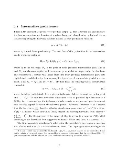
2.3 Intermediate goods sectors
Firms in the intermediate goods sector produce output, y t , that is used in the production of
the …nal consumption and investment goods at home and abroad using capital and labour
services employing the following constant returns to scale production function:
y t = A t f(k t 1; h t ) (15)
where A t is total factor productivity. The cash ‡ow of this typical …rm in the intermediate
goods producing sector is:
t = P Ht A t f(k t 1; h t ) P t w t h t P x;t x t (16)
where w t is the real wage, P Ht is the price of home-produced intermediate goods and P t
and P x;t are the consumption and investment goods de‡ators, respectively. In this baseline
speci…cation, I assume that home …rms turn home-produced intermediate goods into
capital stock, and the foreign …rm uses only foreign-produced intermediate goods for investment.
Thus P x;t = P H;t and Px;t = PF;t . The …rm faces the following capital accumulation
constraint:
k t = (1 )k t 1 + (1 s( x t
x t 1
))x t (17)
where the initial capital stock, k 1 , is given, is the rate of depreciation of the capital stock
and (1 s( xt
x t 1
))x t captures investment adjustment costs as proposed by Christiano et al
(2005), i.e. it summarizes the technology which transforms current and past investment
into installed capital for use in the following period. Following Christiano et al, I assume
that the function s( xt
x t 1
) has the following steady-state properties: s(1) = s 0 (1) = 0 and
s 00 (1) > 0: Schmitt-Grohé and Uribe (2004) suggest the following functional form: s( xt
x t 1
) =
2
x 2.
t
x t 1
1
For the purposes of this paper, all that is needed is a value for s 00 (1), which
according to the functional form suggested by Schmitt-Grohé and Uribe is a constant, : 1
The …rm maximizes shareholder’s value using the household’s intertemporal marginal
rate of substitution as the stochastic discount factor. The Lagrangian corresponding to the
1 It is easy to show that whereas the function (1 s(x t =x t 1 ))x t is not concave for all values of x, it is so
in the vicinity of the steady state, thus the problem is standard in the sense that the conditions (19) - (21)
plus the constraint and the relevant terminal conditions are necessary as well as su¢ cient.
8