Dynamic Meteorology (lecture 5)

10/7/11
Dynamic Meteorology
(lecture 5)
Topics
Fronts and midlatitude cyclones
Life-cycle of a mid-latitude cyclone
Frontogenesis and frontolysis
Q-­‐vector
Pressure as vertical coordinate
Properties of thermal wind balance
Ageostrophic wind
Jetstreak
(a.j.vandelden@uu.nl)
(http://www.phys.uu.nl/~nvdelden/dynmeteorology.htm)
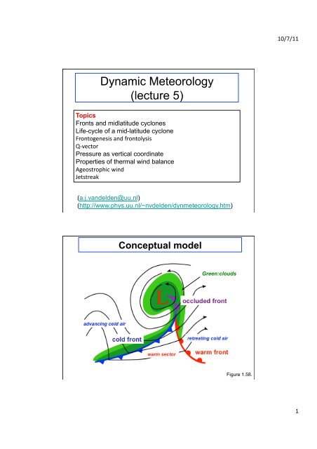
Conceptual model
Green:clouds
Figure 1.58.
1

10/7/11
Weathermap
2

10/7/11
Classical conceptual
models of fronts
Left panel: a cold front. Right panel: a warm front.
(Source: Wikimedia Commons)
The impression is given that less dense warm air is lifted by the
advancing cold air. This is wrong!
Life cycle of mid-latitude
cyclone
Starts with a “wave” in the “Polar Front”. This wave grows due to the
instability of the thermal wind.
a few days Figure 1.59.
3

10/7/11
polar front
time
Why this life-cycle?
Let us first define what a front is in mathematical terms;
Then study mechanisms that lead to the formation of fronts;
Then study mechanisms that lead to the characteristic frontal morphology, seen
in previous slides
Questions about fronts
• What is a front?
• How are fronts formed?
• Why are fronts associated with clouds
• What is the relation between fronts and jetstreams?
4

10/7/11
What exactly is a front?
A front separates two air masses
Air masses are characterized by:
potential temperature, humidity or potential vorticity. Why?
Sometimes gradients of these quantities can be very sharp
Potential vorticity
on 320 K level
(approx. 10 km) in
northern hemisphere on 6
Oct. 2011, 12 UTC.
The standard definition of front-intensity is in terms of temperature
Definition of front-intensity
A front separates two air masses
Suppose:
air masses are characterized by potential temperature,
Intensity of front is measure by
⎛⎛
where ∇ h ≡ ∂ ∂x , ∂ ∂y ,0 ⎞⎞
⎜⎜ ⎟⎟
⎝⎝ ⎠⎠
€
( ∇ h θ) 2
€
5

10/7/11
Frontogenesis function,
Q-vector
€
d( ∇
h θ) 2
= 2Q
⋅∇
h θ
dt
Q ≡ ( Q 1 ,Q 2 ) ≡ d
∇ h θ
dt
Q-vector
If Q-vector is perpendicular to isentrope, potential temperature
gradient increases/decreases.
€
If Q-vector is parallel to isentrope, potential temperature
gradient changes direction (isentrope rotates), but front does
not intensify
Derivation of Q-vector equation
y-component:
2
d ⎛⎛ ∂θ ⎞⎞
⎜⎜ ⎟⎟
dt ⎝⎝ ∂y ⎠⎠
= 2 ∂θ d ⎛⎛ ∂θ ⎞⎞
⎜⎜ ⎟⎟
∂y dt ⎝⎝ ∂y ⎠⎠
€
€
∂ ⎛⎛ dθ ⎞⎞
⎜⎜ ⎟⎟ = ∂ ⎛⎛ ∂θ
∂y⎝⎝
dt ⎠⎠ ∂y ∂t + u ∂θ
∂x + v∂θ ∂y + w∂θ ⎞⎞
⎜⎜
⎟⎟ = 0 (no heating!)
∂z
€
⎝⎝
⎠⎠
⎛⎛ ∂ ∂θ
∂t ∂y + u ∂ ∂θ
∂x ∂y + v ∂ ∂θ
∂y ∂y + w ∂ ∂θ
∂z ∂y + ∂u ∂θ
∂y ∂x + ∂v ∂θ
∂y ∂y + ∂w ∂θ ⎞⎞
⎜⎜
⎟⎟ = 0
⎝⎝
∂y ∂z ⎠⎠
d ∂θ
dt ∂y ≡ Q = −∂u ∂θ
2
∂y ∂x − ∂v ∂θ
∂y ∂y − ∂w ∂θ
∂y ∂z
€
6

10/7/11
Frontogenetic terms
Arrows: streamlines/x-­‐ or y-­‐axis
C:Cold
W:Warm
d ∂θ
dt ∂y ≡ Q 2 = −∂u ∂θ
∂y ∂x − ∂v ∂θ
∂y ∂y − ∂w ∂θ
∂y ∂z
Which of the two
frontogenetic processes
€
shown in the figures is
represented mathematically
in the equation above?
confluence
tilting
Illustration of frontogenesis
Air parcel in
a rotating
fluid*
a
A
b
Suppose:
horizontal solid
lines are
isentropes on a
pressure surface
B
frontogenesis
frontolysis
c
A
B
*flow field is not exactly circularly symmetric
A
B
7

10/7/11
Frontogenesis in baroclinic wave
Model simulation:
blue contours: absolute value
temperature gradient on isobaric
surface (864 hPa).
Red arrows: wind-vector.
(figure 1.63)
30 hours apart
Labels in units of 10 -5 K m -1
Frontogenesis in baroclinic wave
Model simulation:
Blue contours: geopotential height labeled in m (864 hPa)
cyan contours: isotherms on isobaric surface labeled in °C
Red arrows: Q-vector.
(figure 1.62)
8

10/7/11
Q-VECTOR, POTENTIAL TEMPERATURE (cyan) and HEIGHT (blue)
THICK CONTOURS: HEIGHT:1500.0 m; TEMPERATURE: 0.0 °C;
CONTOUR-INTERVAL: HEIGHT: 50.0 m; TEMPERATURE: 5.0 °C
L
rotating isentropes
H
frontogenesis
H
Q-vector in midlatitude depression
pe
model
run 3520
837hPa
: |Q1|=5*10^-11 K m^-1 s^-1 (min. value:10^-11 K m^-1 s^-1)
60.00 hrs
Chain rule: dp = ∂p
∂t
€
On isobaric surface:
Pressure coordinate
Pressure:
dt +
∂p
∂x
€
Without loss of generality:
p( x, y,z,t)
∂p ∂p
dx + dy +
∂y ∂z dz
dp = 0 and ∂p
∂t = 0
dx = 0
€ ∂p ∂p
Therefore: dy +
∂y ∂z dz = 0 ?
€
⎛⎛ ∂p⎞⎞
⎛⎛
⎜⎜ ⎟⎟ = ρg ∂z ⎞⎞ ⎛⎛
⎜⎜ ⎟⎟ ≡ ρ ∂Φ ⎞⎞
⎜⎜ ⎟⎟
⎝⎝ ∂y⎠⎠
z
⎝⎝ ∂y⎠⎠
p
⎝⎝ ∂y ⎠⎠
p
€
€
∂p
dy − ρgdz = 0
∂y
Φ ≡ geopotential
€
€
9

10/7/11
Geostrophic & Hydrostatic
Balance
Geostrophic wind:
Hydrostatic balance:
€
Thermal wind equation:
€
v g = g ⎛⎛ ∂z⎞⎞
⎜⎜ ⎟⎟
f ⎝⎝ ∂x⎠⎠
g = −
p;u g ⎛⎛ ∂z⎞⎞
⎜⎜ ⎟⎟
f ⎝⎝ ∂y⎠⎠
∂p
∂z = −ρg ?
∂v g
∂ln p = − R f
€
p
∂z
∂ln p = − RT g
∂T
∂x ; ∂u g
∂ln p = R ∂T
f ∂y
€
Properties of the thermal wind
*Horizontal derivatives with
pressure held constant
Geostrophic wind:
v g = 1 f
∂Φ
∂x ;u g = − 1 ∂Φ
f ∂y
*
Thermal wind equation:
€
The thermal wind:
€
p ∂v g
∂p = ∂v g
∂ln p = − R f
€
In vector notation:
v T ≡ v
g ( p 1 ) −
v g p
€ 0
∂T
∂x ; p ∂u g
∂p = ∂u g
∂ln p = R ∂T
f ∂y
( ) = − R f
∂ v g
∂ln p = − R f
∫
p 1
p 0
( k ˆ
k ˆ × ∇ T
× ∇ T )d ln p
The thermal wind is parallel to the isotherms!
10

10/7/11
v T ≡ v
g ( p 1 ) − v
g ( p 0 ) = − R f
The thermal wind is parallel to the isotherms!
Turning € of the wind with height
∫
p 1
p 0
( k ˆ
× ∇ T )d ln p
See
problem 1.18
Cold advection: backing with height
Warm advection: veering with height
The thermal wind in a mid-latitude
cyclone
FIGURE 1.60. NOAA image in channel 4
(IR) made on March 3, 1995, at 0157
UTC.
11

10/7/11
The thermal wind in a mid-latitude
cyclone
850 hPa
The thermal wind in a mid-latitude
cyclone
500 hPa
12

10/7/11
v = v
g +
Ageostrophic wind
dv
dt = − f k ˆ × v − ∇ Φ
dv
dt = − f k ˆ × v
a
€
€
v a
€
Ageostrophic wind
v a = 1 f
k ˆ
⎛⎛
× d v ⎞⎞
⎜⎜ ⎟⎟
⎝⎝ dt ⎠⎠
€
geostrophic wind:
fk ˆ × v
g = −∇ Φ
€
v g = 1 k ˆ × ∇ Φ
f
v a = 1 f
⎛⎛
k ˆ × ∂ ⎛⎛
⎜⎜ ⎜⎜
⎝⎝ ∂t ⎝⎝
1
f
Isallobaric wind
⎞⎞
k ˆ × ∇Φ⎟⎟ + ∂ v a
€ ⎠⎠ ∂t + ( v ⋅ ∇) v +ω ∂ v ⎞⎞
⎟⎟
∂p⎠⎠
Inertial-advective wind
Isallobaric wind can sometimes be a very important contribution
€
Example
28 May 2000, 0600 UTC
Thick: isallobaric wind
Thin: geostrophic wind
gray: isobars[hPa]
solid: isallobars[hpa/3hr]
Isallobaric+geostrophic wind
Observed wind
c
13

10/7/11
v a = 1 f
k ˆ
⎛⎛
× d v ⎞⎞
⎜⎜ ⎟⎟
⎝⎝ dt ⎠⎠
d v
dt > 0 €
Jetstreak
d v
dt < 0
€
v a < 0
€
€
v a > 0
€
PROBLEMS
Problems 1.14, 1.15, 1.16, 1.17.
Instead of the case given in the lecture notes, we will do these
exercises for the case of yesterday (6 October 2011): a cold front
passing over the Netherlands. Some of you will analyse the warm
side of the front and others the cold side of the front. You will
calculate quantities such as the geostrophic wind, the vorticity and
divergence.
14

10/7/11
Weathermap
Weathermap
15

10/7/11
Weathermap
Weathermap
16

10/7/11
Weathermap
17

10/7/11
18

10/7/11
19

10/7/11
20

10/7/11
21

10/7/11
FORECAST FROM LAST WEEK
22

10/7/11
Data needed for these exercises
We will use the radiosonde data from six stations:
Ekofisk (01400, 56.5, 3.2), Scheswig (10035, 54.5, 9.5), Hannover
(10238/ETGB, 52.5, 9.7), De Bilt (06260/EHDB, 52.1, 5.2), Essen
(10410/EDZE, 51.4, 7.0) and Meiningen (10548, 50.5, 10.4)
The following slides show the radiosonde-measurements plotted
in a tephigram.
Data needed for these exercises
Hannover/Bergen
Ekofisk
Schleswig
De Bilt
Essen
Meiningen
23

10/7/11
24

10/7/11
25

10/7/11
26

10/7/11
PROBLEM 1.14. Analysis of observations
Compute the 500 hPa wind at the points (x 0 , y 0 )=(5°E, 54°N) and (x 0 , y 0 )=9°E, 51.5°N)
on on 6 October 2011, 12 UTC. First decide which measurements you will use (see the
upper panel of figure 1.54). Compute the 500 hPa isobaric height at the gridpoint (x 0 , y 0 )
=(7°E, 50°N) and (x 0 , y 0 )=(8°E, 56°N). Also compute the isobaric height- and windgradients.
We can use this information to compute the geostrophic wind at 500 hPa
(problem 1.15) and the gradient wind (problem 1.16). The observations and positions of
the measuring stations can be obtained from the following website:
http://weather.uwyo.edu/upperair/sounding.html.
PROBLEM 1.15. Geostrophic wind
Estimate the geostrophic wind (u g , v g ) on 6 October 2011, 12 UTC at the points (x 0 , y 0 )=
(5°E, 54°N) and (x 0 , y 0 )=9°E, 51.5°N) from the gradient of the isobaric height (problem
1.14). Compare the geostrophic wind with the “actual” wind at the same point.
PROBLEM 1.16. Non-linear balance and gradient wind
Calculate the gradient wind from eqs. (1.136) and (1.137) at the points (x 0 , y 0 )=(5°E,
54°N) and (x 0 , y 0 )=9°E, 51.5°N) on the 500 hPa level on 6 October 2011, 12 UTC with
the velocity- and height gradients calculated in problem 1.14. Compare the gradient wind
with the geostrophic wind (problem 1.15).
PROBLEM 1.17. Relative vorticity and horizontal divergence
Estimate the relative vorticity and the horizontal divergence on the 500 hPa isobaric
level on 6 October 2011, 12 UTC at the points (x 0 , y 0 )=(5°E, 54°N) and (x 0 , y 0 )=9°E,
51.5°N) with the velocity gradients calculated in problem 1.16. Compare the relative
vorticity with the planetary vorticity. Also give an estimate of the Rossby number (section
1.23). Compare the horizontal divergence at the two points (eq. 1.138b).
27

10/7/11
5 groups of 2: 3 doing the cold side, of which one is using the
measurement of Nordeney and the other two of Schleswig
(respectively, 700 and 500 hPa).
Other two do the warm side (respectively, 700 and 500 hPa).
Each group shortly presents the results next week (Friday
afternoon, 14 October 2011)
28