Answers to Homework #7 - Statistics

Homework #7 solutions
Stat 640
1. True. Let the columns of X 0 be a basis for V 0 . Then the projection of y onto V 0
is
Π(y|V 0 ) = X 0 (X ′ 0X 0 ) −1 X ′ 0y
= X 0 (X ′ 0X 0 ) −1 X ′ 0ŷ + X 0(X ′ 0X 0 ) −1 X ′ 0(y − ŷ)
and the second term on the right is zero because the columns of X 0 are contained
in V and hence orthogonal to y − ŷ.
2. Let the parameter vector be (β, α 1 , α 2 , α 3 ), where β is the joint slope and the αs
are the expected dry weights for the middle fertilizer amount. (Note that we use
the “centered” coding for fertilizer values. We will find simultaneous confidence
intervals for η = c ′ β where c 1 = 0 and c 2 + c 3 + c 4 = 0. Thus, q = 2. Because
of the way we have coded the variables, X ′ X is a diagonal matrix with values
10, 5, 5, 5. For any of the desired pair-wise contrasts, we have c ′ (X ′ X) −1 c = 2/5,
and F .95 (2, 11) = 3.98. For these data, we get√S = 2.612 so that we can compare all
pairwise differences in the α parameters to S qc ′ (X ′ X) −1 cF 0.95 (q, n − k) = 4.66.
The estimates are α 1 = 45.4, α 2 = 46.8, and α 3 = 50.6. Therefore, we find that
the expected dry weights using soils A and C are significantly different.
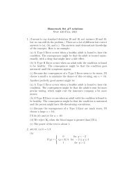
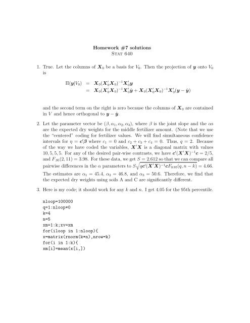
3. Here is my code; it should work for any k and n. I get 4.05 for the 95th percentile.
nloop=100000
q=1:nloop*0
k=4
n=5
xm=1:k;xv=xm
for(iloop in 1:nloop){
x=matrix(rnorm(k*n),nrow=k)
for(i in 1:k){
xm[i]=mean(x[i,])

xv[i]=var(x[i,])
}
sp=mean(xv)
dmax=0
for(i in 1:(k-1)){
for(j in (i+1):k){
dist=abs(xm[i]-xm[j])
if(dist>dmax){dmax=dist}
}
}
q[iloop]=dmax/sqrt(sp/n)
}
hist(q)
sort(q)[95000]
Histogram of q
Frequency
0 10000
0 2 4 6 8 10
q
4. Whatever j we choose, we will have µ = (6, . . . , 6, 10, . . . , 10, 12, . . . , 12, 8, . . . , 8) ′ ,
so that µ 0 = (8, . . . , 8, 10, . . . , 10) ′ and ‖ µ − µ 0 ‖ 2 = 16j. Then δ = 16j/4 = 4j.
The critical value for the test is F 0.95 (2, 4(j − 1)). Let’s try some values of j.
For j = 3, we have F 0.95 (2, 8) = 4.459, δ = 12, and P (F > 4.459) = .72 under H a .
For j = 4, we have F 0.95 (2, 12) = 3.885, δ = 16, and P (F > 3.885) = .89 under

H a .
For j = 5, we have F 0.95 (2, 16) = 3.634, δ = 20, and P (F > 3.634) = .96 under
H a .
5. We have µ = (16, . . . , 16, 20, . . . , 20) ′ , where there are 2j elements equal to 16 and
3j elements equal to 20, and µ 0 = (18.4, . . . , 18.4) ′ . ‖ µ − µ 0 ‖ 2 = 19.2j. Then
δ = 19.2j/25 = .768j.
For j = 5, we have F 0.95 (4, 20) = 2.866, δ = 3.84, and P (F > 2.866) = .25 under
H a .
For j = 10, we have F 0.95 (4, 45) = 2.579, δ = 7.68, and P (F > 2.579) = .53 under
H a .
For j = 20, we have F 0.95 (4, 95) = 2.467, δ = 15.36, and P (F > 2.467) = .88 under
H a .
For j = 17, we have F 0.95 (4, 80) = 2.486, δ = 13.01, and P (F > 2.579) = .81 under
H a .
6. (a) Let β 0 be the expected mercury measurement at the plant, let β 1 be the
downstream rate of increase of mercury, and let β 2 be the upstream rate of increase
of mercury. Suppose the measurements are ordered so that y 1 is the measurement
two kilometers downstream, y 9 is the measurement two kilometers upstream, and
the others are consecutive up the river. Then y = Xβ + ɛ, where β = (β 0 , β 1 , β 2 ) ′
and
⎛
⎞
1 2 0
1 1.5 0
1 1 0
1 .5 0
X =
1 0 0
.
1 0 .5
1 0 1
⎜
⎟
⎝ 1 0 1.5 ⎠
1 0 2
(b) H 0 : β 1 = β 2 = 0; H a : at least one is not zero.

(c) Let SSE 0 be ∑ 9
i=1 (y i − ȳ) 2 , the sum of squared residuals under H 0 . Let SSE 1
be sum of squared residuals under the full model in (a). Then
F = (SSE 0 − SSE 1 )/2
SSE 1 /6
is distributed as F (2, 6) if the null hypothesis is really true.
(d) If the environmentalist are correct,
E(y) = µ = (75, .8125, .875, .9375, 1, .875, .75, .625, .5) × 800
= (600, 650, 700, 750, 800, 700, 600, 500, 400).
For the null hypothesis µ 0 , we project µ onto the one-vector, to get (633.33)1,
and ‖ µ − µ 0 ‖ 2 = 125000. The estimate of the model variance is σ 2 = 100, so
δ = 1250. We will reject H 0 if our F -statistic is greater than F 0.95 (2, 6) = 5.143.
The power of the test is about one!