Answers to Homework #5 - Statistics

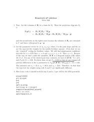
# code to simulate the null distribution of Fmax when the
# sample sizes are 12, 8, 10, 10, 14.
svec=1:5
nloop=100000
fmax=1:nloop*0
nj=c(12,8,10,10,14)
for(i in 1:nloop){
for(j in 1:5){
x=rnorm(nj[j])
svec[j]=var(x)
}
fmax[i]=max(svec)/min(svec)
}
0 10 20 30 40
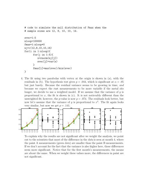
4. The fit using two parabolas with vertex at the origin is shown in (a), with the
residuals in (b). The hypothesis test gives p = .044, which is significant at α = .05
but just barely. Because the residual variance seems to be growing in time, and
because we expect the rust measurements to be more variable if the metal sits
longer, we decide to use a weighted model. If we assume that the variance of y is
proportional to x, the fit is shown in (c). It is not noticeably different than the
unweighted fit; however, the p-value is now p = .074. The residuals look better, but
now let’s assume that the variance of y is proportional to x 2 . The fit again looks
very similar, but now we get p = .141.
(a)
res
-5 0 5
(b)
y
0 10 20 30 40
(c)
restr
-4 -2 0 2 4
(d)
restr
-2 -1 0 1 2
(e)
1.0 1.5 2.0 2.5 3.0 3.5 4.0
1.0 1.5 2.0 2.5 3.0 3.5 4.0
1.0 1.5 2.0 2.5 3.0 3.5 4.0
1.0 1.5 2.0 2.5 3.0 3.5 4.0
1.0 1.5 2.0 2.5 3.0 3.5 4.0
To explain why the results are not significant after we weight the analysis, we point
out to the scientists that most of the difference in the data is seen at month 4, where
the paint A measurements (green dots) are smaller than the paint B measurements.
If we don’t account for the fact that the variance is also higher here, these differences
seem more significant. Notice that for the first month’s measurements, the means
are about the same. When we weight these values more, the differences in paint are
not significant.