Errata for Computational Statistics, 1st Edition, 2nd Printing

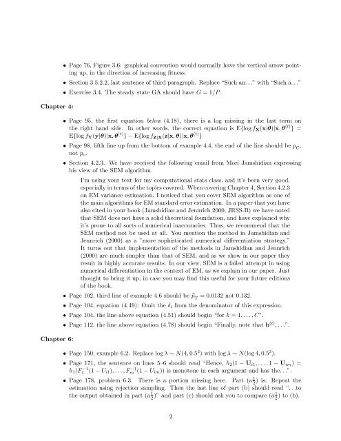
Chapter 4:
Chapter 6:
• Page 76, Figure 3.6: graphical convention would normally have the vertical arrow pointing
up, in the direction of increasing fitness.
• Section 3.5.2.2, last sentence of third paragraph. Replace “Such an...” with “Such a...”
• Exercise 3.4. The steady state GA should have G = 1/P.
• Page 95, the first equation below (4.18), there is a log missing in the last term on
the right hand side. In other words, the correct equation is E{logf X (x|θ)|x,θ (t) } =
E{logf Y (y|θ)|x,θ (t) }−E{logf Z|X (z|x,θ)|x,θ (t) }
• Page 98, fifth line up from the bottom of example 4.4, the end of the line should be p C
,
not p c .
• Section 4.2.3. We have received the following email from Mori Jamshidian expressing
his view of the SEM algorithm.
I’m using your text for my computational stats class, and it’s been very good,
especiallyintermsofthetopicscovered. WhencoveringChapter4, Section4.2.3
on EM variance estimation, I noticed that you cover SEM algorithm as one of
the main algorithms for EM standard error estimation. In a paper that you have
also cited in your book (Jamshidian and Jennrich 2000, JRSS-B) we have noted
that SEM does not have a solid theoretical foundation, and have explained why
it’s prone to all sorts of numerical inaccuracies. Thus, we recommend that the
SEM method not be used at all. You mention the method in Jamshidian and
Jennrich (2000) as a ”more sophisticated numerical differentiation strategy.”
It turns out that implementation of the methods in Jamshidian and Jennrich
(2000) are much simpler than that of SEM, and as we show in our paper they
result in highly accurate results. In our view, SEM is a failed attempt in using
numerical differentiation in the context of EM, as we explain in our paper. Just
thought to bring it up, in case you may find this useful for your future editions
of the book.
• Page 102, third line of example 4.6 should be ̂p T
= 0.0132 not 0.132.
• Page 104, equation (4.49): Omit the δ i from the denominator of this expression.
• Page 104, the line above equation (4.51) should begin “for k = 1,...,C”.
• Page 112, the line above equation (4.78) should begin “Finally, note that b (t) ,...”.
• Page 150, example 6.2. Replace logλ ∼ N(4,0.5 2 ) with logλ ∼ N(log4,0.5 2 ).
• Page 171, the sentence on lines 5–6 should read “Hence, h 2 (1 − U i1 ,...,1 − U im ) =
h 1 (F1 −1 (1−U i1 ),...,Fm −1 (1−U im )) is monotone in each argument and has the...”.
• Page 178, problem 6.3. There is a portion missing here. Part (a 1 2
) is: Repeat the
estimation using rejection sampling. Then the last line of part (b) should read “...to
the output obtained in part (a 1 2 )” and part (c) should ask you to compare (a1 2
) to (b).
2