A Linear Mixed Effects Clustering Model for Multi-species Time ...

DEPARTMENT OF STATISTICS
University of Wisconsin
1300 University Avenue
Madison, WI 53706
TECHNICAL REPORT NO. 1143
July 10, 2008
A Linear Mixed Effects Clustering Model for Multi-species Time
Course Gene Expression Data 1
Kevin H. Eng
Department of Statistics
University of Wisconsin, Madison
Sündüz Keleş
Department of Statistics
Department of Biostatistics and Medical Informatics
University of Wisconsin, Madison
Grace Wahba
Department of Statistics
Department of Biostatistics and Medical Informatics
University of Wisconsin, Madison
1 This work was supported by NSF grant DMS-0604572 (GW), ONR N0014-06-0095 (GW), a PhRMA
Foundation Research Starter Grant (SK) and NIH grants HG03747-01 (SK) and EY09946 (GW)

Abstract
Environmental and evolutionary biologists have recently benefited
from advances in experimental design and statistical analysis for complex
gene expression microarray experiments. The high-throughput
time course experiment highlights gene function by uncovering functionally
similar responses across varied experimental conditions. Since
these time-dependent responses can be compared across phylogenetic
branches, we argue that the extension to multi-factor designs incorporating
closely related species adds an evolutionary context to the
analysis as well as being of considerable interest in its own right. Motivated
by time course gene expression experiments conducted over
multiple strains of yeast, we propose a mixed effects model based
clustering method that preserves the factor information contained in
time and in species. The result is a partitioning of the common, homologous
genome into functional groupings cross-tabulated by their
response in different species and annotated by their mean effects and
dependence in time and over phylogeny. In a set of experiments containing
yeast species in the Saccharomyces sensu stricto complex, we
give examples of detectable patterns and describe inferences of interest
on their estimated covariances. We demonstrate via simulation that a
mixed effects type model has good clustering properties and is robust
to noise.
Keywords: Comparative biology; Cluster analysis; Gene expression;
Linear mixed models; Microarrays; Mixture models; Time course
gene expression.
1

A Linear Mixed Effects Clustering Model for
Multi-species Time Course Gene Expression
Data
Kevin H. Eng, Sündüz Keleş ∗ , and Grace Wahba
Department of Statistics,
Department of Biostatistics and Medical informatics,
University of Wisconsin-Madison,
1300 University Ave., Madison, WI 53706, USA.
*keles@stat.wisc.edu
July 10, 2008
1 Introduction
Understanding the mechanisms behind the evolution of gene function is a
major challenge in evolutionary biology. While biologists have traditionally
studied genes’ biochemical and structural functions based on the variations
in coding sequences, many studies have argued and demonstrated that a
gene’s function can also be defined by its role in specific cells, tissues, organs,
genetic pathways and whole organisms. The study of gene expression traits
connects these higher order phenotypes to the information contained in the
genome. With the advent of microarray technology, it is possible to measure
and identify expression differences within and among species across whole
genomes (Rifkin et al., 2003; Fay et al., 2004; Khaitovich et al., 2004; Gilad
et al., 2006; Whitehead and Crawford, 2006).
Variations in expression have been long recognized as a fundamental part
of the process of evolution (Britten and Davidson, 1969; King and Wilson,
1975; Wray et al., 2003); King and Wilson (1975) argued 30 years ago that
differences in gene regulation may be responsible for differences between
2

closely related species. Naturally, early cross-species microarray studies investigated
differences unexplainable by DNA coding sequence, measuring
expression under various experimental conditions. Gilad et al. (2006), for
example, compared gene expression in liver tissue within and between humans,
chimpanzees, orangutans and rhesus macaques and, consistent with
King and Wilson’s hypothesis, identified of a set of human-specific genes
encoding transcription factors, DNA binding proteins.
With the maturation of microarray technology, comparative experiments
are increasingly common, leading evolutionary biologists to a curious sort of
induction: instead of single genes they must contend with information from
entire genomes. Aggregating expression over different Drosophila lines, Rifkin
et al. (2003) argue that the percentage of genes showing expression divergence
is a useful measure of evolutionary distance versus the divergence in sequence
of a few select genes. Whitehead and Crawford (2006) state that the effects of
balancing selection are easily identified in different populations of Fundulus
heteroclitus since the microarrays simultaneously measure a sufficient number
of genes to provide a proper estimate of gene-wise variation.
The result is the ability to consider evolutionary hypotheses at the level
of single genes distinguished from thousands of patterns across the whole
organism. The previous two studies, as well as Khaitovich et al. (2004) and
Nuzhdin et al. (2004), are particularly interested in testing Kimura’s (1991)
neutral drift (neutral evolution) hypothesis on each gene, which states that
the correlation in a particular trait between species is inversely proportional
to the phylogenetic distance between them. This neutral evolution theory
implies a particular structure (a phylogenetic tree), and, for multivariate normal
traits, it can be argued that the signature of evolution may be observed
in a tree-structured covariance matrix (Gu, 2004; McCullagh, 2006).
All of these studies involve a small number of species measured over only
a few experimental conditions and are therefore conveniently analyzed with
well established statistical tools (Kerr and Churchill, 2001; Smyth et al.,
2003). A common extension of single condition experiments is to profile
expression over a time course (Chu et al., 1998; Bar-Joseph et al., 2002; Luan
and Li, 2003; Storey et al., 2005; Yuan and Kendziorski, 2006; Qin and Self,
2006; Tai and Speed, 2006). While conventional gene expression analysis can
associate individual genes with a single condition (e.g., tissue type or habitat
temperature), a time course gene expression analysis ties genes together into
functional groups and prompts their association with underlying biological
processes. Such processes can be natural cycles (Spellman et al., 1998), or
3

they can be a response to a stimulus as in the yeast Environmental Stress
Response (Gasch et al., 2000).
In these analyses, the assumption is that genes which are correlated with
one another are likely represent functional groups and the goal is to uncover
these biological clusters. Among the clustering models for time course gene
expression data, model based clustering (Fraley and Raftery, 2002) is widely
used because it provides a flexible and adaptive alternative to nonparametric/algorithmic
clustering techniques (k-means or hierarchical clustering). In
particular, the regression clustering models in Qin and Self (2006) use the
time factor to model the observed signal leading to interpretable regression
coefficients and variances and to facilitate formal hypothesis testing. In particular,
with the incorporation of random effects terms (Luan and Li, 2003;
Ng et al., 2003; Qin and Self, 2006) these models can accommodate higher
levels of heterogeneity among expression profiles of individual genes and can
induce correlations among expression levels across different time points.
Although, the literature of well-studied statistical models for single species
experiments is considerable, their multi-species counterparts have not fully
emerged. Ideally, new models incorporating species components to gene expression
studies will admit the analyses we highlighted above: tests of natural
selection hypotheses versus neutral drift and the ability to study gene specific
phylogenies, “gene trees,” in detail. In this article, we develop a framework
for analyzing multi-species time course gene expression experiments based
on a comparative (i.e., across species) linear mixed effects clustering model.
Our proposed approach produces significant gains over existing methods by
carefully balancing the functional implications of the time factor with the
evolutionary implications of the species factor. We compare and contrast
model based clustering and regression clustering models which differ based
on their parameterizations of the mean expression profiles across the time
course and across strains. We discuss fitting issues, conduct simulation studies
comparing the relative performances of other clustering models on this
type of data, and give the results of an analysis on a multi-species yeast heat
shock stress response data set.
4

2 Methods
2.1 Clustering Model
In the time course gene expression experiment, it is of interest to group
genes together by their common structure over time since genes with similar
time profiles may have similar biological functions. A naive approach is
to model each gene with its own linear model and to test or cluster the
coefficients into similar patterns. Instead of a model for every gene, Qin and
Self’s class of clustering of regression models (2006) assumes that every gene
measured belongs to a class defined by a linear mixed effects model with a
random effect for time. Genes in the same class share the same mean time
profiles and the same longitudinal dependence structures. The net effect is
a more parsimonious representation of the experiment and a greater number
of observations (entire genes) available for estimation. We intend to extend
this model to incorporate an additional random effect for species.
In the multi-species time course experiment, we measure gene expressions,
Y gsti , for observation i = 1, . . . , N of species s = 1, . . . , S at time t = 1, . . . , T
for each gene g = 1, . . . , G. For simplicity, we assume that each species is
measured on the same set of time points, that the species are sufficiently
similar to allow us to measure a set of comparable orthologs. Then, observations
for each gene are contained in Y g ∈ R ST N×1 . The naive approach
models each of these vectors individually with a per-gene linear mixed effects
model,
Y g = Xβ g + W a g + Mb g + ɛ g , (1)
where β g ∈ R T S×1 are gene specific fixed effects, a g ∈ R T ×1 are random effects
in time and b g ∈ R S×1 are random effects across species with appropriate
design matrices X, W , M. While this model assumes that each gene has
its own mean and covariance, the assumption is often impractical because
the number of observations of any single gene are few and it is of interest to
exploit common structures between functionally similar genes.
We choose, therefore to follow Qin and Self (2006) and to designate k =
1, . . . , K component models. For gene g, let U g ∈ {1, . . . , K} be the clustering
variable. The model for a complete vector, Y g , in cluster k, is given by:
Y g | {U g = k} = Xβ k + W a gk + Mb gk + ɛ gk , (2)
where the fixed effects (β k ) and random effects (a gk and b gk ) are now cluster
5

specific. That is, we assume that
a gk = a g | {U g = k} ∼ N (0, A k ),
b gk = b g | {U g = k} ∼ N (0, B k ), (3)
ɛ gk = ɛ g | {U g = k} ∼ N (0, σ 2 kI),
are conditionally independent multivariate normal random variables where
the covariance matrices A k are of dimension T × T and B k are S × S, both
of unspecified structure. Under these assumptions, a gene from cluster k has
the following marginal distribution:
Y g | {U g = k} ∼ N (Xβ k , V gk ) , (4)
V gk = W A k W ′ + MB k M ′ + σ 2 kI. (5)
In this model, the cluster centers are the regression coefficients, β k , or equivalently
the mean time profiles over all species, Xβ k . This means that genes
showing common species specific differences (as well as common time patterns)
will tend to group together into the same cluster. Then, each component
represents a unique functional pattern and instead of describing each
gene as a mixture, the model tries to assign the gene to a single cluster. In
practice, goodness of fit can be assessed by considering the clustering certainty,
hopefully each gene is ascribed to only one cluster with high posterior
probability.
Our model can be reduced to other mixed effects clustering models with
species components such as Ng et al. (2003), who propose a multiple random
effects model but use only diagonal covariances. In a data set where
there are many time points, it may be fruitful to consider spline models
over time, as in Luan and Li (2003), who use B-spline bases to model both
fixed and random effects for time course data. In a paper to appear shortly,
Ma and Zhong (2008) propose a functional (a.k.a smoothing spline) ANOVA
model with smoothing splines for time course cluster means and random effects
covariates which could model a species factor, treated as part of the
loss function. In the sense that model based clustering (Mclust) (Fraley and
Raftery, 2002) parameterizes the variance of a gaussian component through
the eigenvector decomposition, clustering of regression models (Qin and Self,
2006) parameterize both the mean and variance. Our clustering of mixed
effects models further parameterizes the variance terms taking advantage of
the covariate information. These regression models can be less parsimonious
than the simplest Mclust models but they add parameters which are of particular
interest.
6

2.2 Structured Covariances
Using two random effects separates correlation attributable to time points
A k from correlation between species B k . In this article, we assume only
that these matrices are positive definite, but the model may be adapted for
any structured form. For example, if we wish to impose an autoregressive
scheme in time we may use the formulation in McCulloch and Searle (2001)
(pp. 193, 201) for A k and derive an estimating equation for the autoregressive
parameters. Generally, the matrix B k is a representation of the branching
structure of a Brownian motion diffusion process describing an evolutionary
history (Felsenstein, 1973), and the estimation we describe admits two types
of analysis important to evolutionary biology.
In phylogenetic analyses, the tree-structured form of B k (McCullagh,
2006) is of interest and predicted random effects E(b gk |Y g , U g ) represent corrections
to expression due to the species factor (phylogeny). Corrada Bravo
et al. (2008) argue that estimating B k under tree-structured constraints admits
a gene expression derived phylogenetic effect. The estimate may be
compared against a sequence derived covariance in order to determine deviation
from neutral drift. As a practical procedure, consider a predefined set
of “pseudogenes” (Khaitovich et al., 2004), genes for which there ought to
be no force of selection. The covariance estimated on the set of psuedogenes
might be used as an estimate of the neutral drift covariance for hypothesis
testing.
In comparative analyses, the matrix B k is a nuisance parameter typically
estimated from DNA sequence data. Freckleton et al. (2002) argue that the
primary interest in modeling this dependence is to make better inferences
about β k , so it is not unreasonable to attempt to estimate B k directly from
expression data. Alternative models of note are the modeling procedure described
in Guo et al. (2006) which chooses among 3 possible parameterized
versions of B k to find a good correction for the observed phylogenetic dependence,
and a similar formulation in Eng et al. (2008) which estimates a
mixing proportion to control a continuum of corrections.
2.3 Model Fitting
In a given experiment, we only observe Y g ; therefore we treat U g , a gk , and
b gk as missing data and apply the Expectation-Maximization (EM) algorithm
(Dempster et al., 1977), described in Appendix A, to fit the model. Because
7

the EM algorithm is known to be sensitive to the choice of initial starting
values (McLachlan and Krishnan, 1996), instead of a random initialization,
we seed the model with a per-gene analysis, an exploratory clustering method
“Mclust on coefficients” described in later sections.
Gene pre-screening. Since we are only interested in genes that show at
least some time dependent effect, we can pre-screen the genes by fitting a
fixed effects ANOVA model with time and species factors to each gene and
then removing genes with insignificant main effects for time. Pre-screening
on F-statistics admits some false discovery rate (FDR) control, but we note
that the assumption of a heterogeneous covariance structure is inconsistent
with the standard ANOVA application and we expect that the F-statistics
may lose some control of the FDR. As we will demonstrate in the simulation
section, it turns out that making false positive errors here is not too dramatic
since the clustering model seems to be able to identify and isolate singleton
noise. Therefore, it is generally advisable to choose a pre-screening threshold
based on the maximum number of genes of interest or based on a target
FDR somewhat larger than usual, and to test the time effect hypothesis
after clustering.
Choosing the number of clusters. It has been argued that using BIC
(Schwarz, 1978) is appropriate to choose the number of components in a finite
mixture even though mixtures violate the standard regularity conditions for
likelihood methods (Fraley and Raftery, 1998). Especially for models which
parameterize the variance, we find that BIC is too strict in that it favors a
small number of components in cases when graphical checks and biological
insight suggest otherwise (Eng et al., 2007). Suppose that p µ and p Σ are
the number of parameters associated with the mean and variance of a single
component respectively and ll(K) = log L(θ K ; Y |K) is the log likelihood fit
for K clusters. Then BIC(K) = −2ll(K) + K(log n)(p µ + p Σ ) favors K + 1
components over K when BIC(K + 1) < BIC(K) or
ll(K + 1) − ll(K) > (log n)(p µ + p Σ )/2, (6)
L(θ K+1 ; Y |K + 1)
L(θ K ; Y |K)
> n (pµ+p Σ)/2 . (7)
Here, we observe the convention in Fraley and Raftery (1998) of not adding
the mixing proportion to the set of free parameters. In order for a mixture to
choose K + 1 components versus K, the improvement in log likelihood must
overcome the penalty for all the parameters associated with a component’s
8

mean and variance. Thus, there is some tradeoff between the complexity in
the component level model (particularly the covariance) and the number of
components. Recalling that this preference for simple models is a standard
property of BIC, we would ideally want to enforce a parsimonious representation
in the number of components (K) that fairly penalizes component
model complexity (p µ and p Σ ); we want a criterion that gives equal penalty
to simple covariances and to complex covariances.
In practice, models with too few clusters can be detected by inspection
since clusters will appear too heterogeneous while models with too many
clusters might appear to have clusters which could be combined. Intuitively,
if two components are similar but have different means, it may be less costly
to combine the two clusters inflating their single covariance. Qin and Self
(2006) may have similarly observed this problem since they suggested a combination
of BIC, for a good predictive fit, and the maximum of the bootstrapped
largest eigenvalues of the cluster covariance matrices (the BMV -
bootstrapped maximum volume), penalizing this over-dispersion.
A standard alternative to BIC might be to choose the number of clusters
based on cross validated likelihood; that is, we can choose the number of
components in the mixture based on estimated out of sample prediction
performance. For a mixture, it is natural to use the negative log likelihood
as a loss function (van der Laan et al., 2004).
In the next section, we demonstrate the application of this model to a data
set with multiple species of yeast measuring their temporal response to heat
shock. In later sections we will demonstrate that accounting for structured
heterogeneity in observations leads to better clustering results even in the
presence of large variances and un-clusterable, singleton noise.
3 Data Analysis
Tirosh et al. (2006) measured the response to heat shock in four species of
yeast on two-channel DNA microarrays by arraying a sample from each time
point against a baseline measurement from the same culture. So, the log
ratio measurements represent a relative change due to stress over time. For
illustration of a complex interspecies design, we combine this data set with an
analogous heat shock experiment over 5 strains of Saccharomyces cerevisiae
from the Gasch Lab at Wisconsin (Eng et al., 2008).
In total, there are 6 strains of S. cerevisiae (S288C, K9, M22, RM11a,
9

YPS163, BY4743), 2 strains of S. paradoxus (CBS432 and NRRL Y-17217)
and one each of S. kudriavzevii and S. mikatae representing 4 closely related
species. The strains are measured over 9 time points (5, 10, 15, 20, 30, 45, 60,
90, 120 minutes post heat shock) with 110 total arrays (60 from the Gasch
Lab and 50 from Tirosh et al. (2006)). We normalize within arrays, and quantile
normalize arrays taken at the same time points. The normalization of
arrays across laboratories is a current research topic elsewhere (Consortium,
2005) and not addressed further in this article.
[Figure 1 about here.]
Each study’s arrays measure over 5000 yeast genes of which 3542 genes
have orthologous sequences in every species. As described in Section 2.3,
pre-screening the genes with a per-gene two way ANOVA model selects 2606
genes with significant time patterns (FDR < 0.01).
[Table 1 about here.]
Using Mclust’s mixture of gaussians to cluster the log ratios directly yields
a mixture of 48 components with the same diagonal covariance by BIC. Due
to the dimension of the data, Mclust can only search through its predefined
“diagonal” and “spherical” covariance models (Fraley and Raftery, 2002). In
Table 1, we list the best K for each of the available models. We only consider
Mclust models which add p µ mean and p Σ covariance parameters per cluster,
omitting the models which share parameters across clusters. Note that for
these alternatives, K = 48 is the largest number of components estimable.
A first approximation of a clustering of regressions model may be fit by
applying Mclust to the coefficients of the per-gene ANOVA models. Since
the coefficients represent a transformation of the data, this is a reasonable
exploratory procedure (analogous to how Mclust uses hierarchical clustering
to choose its seed assignments, Eng et al. (2007)). It is somewhat more fair
than the vanilla Mclust since it only considers the covariance between group
means. BIC values from this model fit are not directly comparable to the
other procedures. This procedure chooses K = 82 components which we
use as an upper limit for the number of clusters. Applying agglomerative
clustering to the cluster centers, for every K ≤ 82, we may seed the mixed
effects clustering model by assigning genes to clusters based on which clusters
collapse together for a particular K.
10

Table 1 includes BIC values for K = 5, the choice if we follow BIC
strictly, and K = 12, the choice if we follow cross-validated likelihood (CV)
which minimizes out of sample prediction error. Choices for K by the usual
Mclust procedure as well as the Mclust on coefficients procedure are also
tabulated. In all cases, the BIC criterion for the mixed effects model is
much smaller than all of the Mclust models implying any one of the mixed
effects models is a better fit. This is, of course, not surprising since we use
covariate information to improve the model fit (p µ = 110 for Mclust models
while p µ = 18 for mixed effects models). The count of component specific
parameters p µ and p Σ are included in the table to illustrate the magnitude
of the BIC penalty for adding a single component. It is not clear which
result we should favor; by inspection we find K = 5, 12 too coarse (median
524,298 genes per cluster) and even at K = 48 clusters are still relatively
large (median x genes per cluster). For illustration, we present the results
for K = 82 (24 genes per cluster), chosen by Mclust on coefficients, later in
this section.
Beyond information criteria, a primary tool in evaluating the goodness
of the clustering model fit is a high resolution heat map plot. For plots
comparing a best Mclust fit, a comparable hierarchical clustering fit and a
selection of linear mixed effects clustering model fits, see the Supplementary
Figures 1-6 online. We can also determine goodness of clustering by considering
a silhouette type plot (van der Laan and Bryan, 2001). Since one of
the byproducts of the EM fit is a posterior probability of cluster membership
we sort genes by their cluster assignment and their posterior probability of
being in that cluster. Supplementary Figure 7 shows that, for the mixed
effects clustering model, nearly all genes (2575 / 2606) have greater than 0.5
posterior probability of being in their assigned class, a good clustering result.
More specifically, we may investigate interesting clusters through their
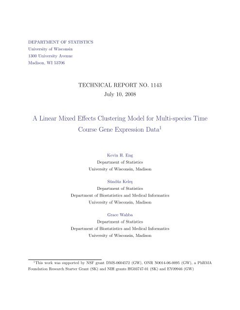
fitted time patterns. In Figure 1, we plot one cluster with a consistent time
pattern representative of a single function. The 47 genes in this cluster are
strongly associated with Gene Ontology (GO) biological process “ubiquitindependent
protein catabolic process” (GO:0006511, 26 of 113 genes present,
p < 1×10 −14 ); GO molecular function “endopeptidase activity” (GO:0004175,
21 of 28 genes present, p < 1 × 10 −14 ); and several GO cellular components,
particularly “20S core proteasome” (GO:0005839, 13 of 15 genes present, p <
1×10 −14 ) via geneontology.org, yeastgenome.org and funspec.med.utoronto.ca.
Ubiquitin, endopeptidase and the 20S proteasome have well characterized
roles in the detection of damaged proteins and their degradation during cel-
11

lular stress. We might interpret this effect as a sudden increase, in response
to heat shock, in the production of genes which identify and eliminate damaged
proteins followed by a rapid return to some new equilibrium state. The
magnitudes of the new equilibrium are different, in particular, the profiles
show a similar specific effect in the M22 strain of S. cerevisiae and the S.
mikatae strain. We can hypothesize that both of these require a large (net
positive) increase in the resting expression of genes associated with this process.
M22, for example, is known to grow poorly at 37C so a higher rate of
ubiquitin production may be a compensatory mechanism. These 47 genes appear
together in the same cluster (along with other genes) for every K ≤ 82
suggesting a reasonably consistent clustering result.
Further downstream analysis utilizes the attributable phylogenetic effect,
the predicted random effects (b gk ) of the species under study. We interpret
these as the component of the observed signal that can be attributed to the
underlying dependence due to species factors alone, independent of time.
For the cluster of 47 genes above, we find the closest sum-absolute-value
norm tree corresponding to the estimated covariance ( ˆB k ) (Corrada Bravo
et al., 2008), building a gene expression based tree (Figure 2). The tree estimate’s
first split places 5 of 6 S. cerevisiae strains together, a reasonable
result (strains should be more similar than species), however the difference
is confounded by which lab prepared the assay. Labs are denoted (G) for
Gasch Lab and (B) for the Barkai lab from Tirosh et al. (2006). For comparison,
Figure 2 also provides the sequence derived tree using DNA sequence
from a sample of upstream coding regions of the strains in the study. Since
S. paradoxus CBS432 has not been sequenced, we place it along-side the
other paradoxus strain. This estimate represents the species tree since it
samples from homologous sequences. Further, since it uses DNA sequence
information, it is not confounded with the laboratory effect. Trees estimated
from sequence and expression data play a role in the comparative analysis
described in Eng et al. (2008).
[Figure 2 about here.]
12

4 Simulation Studies
4.1 Candidate Models
In order to investigate the advantages of explicitly accounting for different
experimental factors and their induced correlations, we consider two applications
of Mclust models (Fraley and Raftery, 2002) and two fixed effects
models. All of the methods are similar in that they model the marginal
distribution of a gene in a particular cluster and they each assume that
U g ∼ Multinomial(π k ). The letters preceding the model are the plot abbreviations.
1. Mclust on data. This clustering method is one step removed from
hierarchical clustering in that it gives parametric form to the clusters,
allows the calculation of BIC for determining the number of clusters and
admits a measure of “uncertainty” about cluster membership. Mclust’s
standard application fits the best model from a set of covariance matrices
parameterized by their eigenvector decomposition. The mean vector
µ k is ST N × 1, and the cluster specific distributions, for k = 1, . . . , K,
are given by:
m1 : Y g | {U g = k} ∼ N (µ k , Σ k ). (8)
2. Mclust on coefficients. This is a natural, ad hoc procedure for the
exploratory analysis (Eng et al., 2007). It is an extension of the pergene
approach: we fit gene-wise ANOVA models and use Mclust on
the estimated coefficients. Since we consider only the estimates, the
procedure represents model based clustering on a transformation of
the data. The parameter vector β g is (S + T − 1) × 1 and the model
for cluster k = 1, . . . , K is:
m2 : β g | {U g = k} ∼ N (b k , Σ k ). (9)
3. Fixed effects models. We consider two types of fixed effects models.
The first is a natural application of clustering of regression models,
equivalent to Qin and Self (2006)’s fixed effects CORM model. The
second is an analog of the generalized least squares model, we include
a more general covariance allowing it to range freely with no specific
structure due to factors. In these cases the vector β k is (S + T − 1) × 1.
13

Then, we have the following cluster specific models, respectively for
k = 1, . . . , K:
fx1 : Y g | {U g = k} ∼ N (Xβ k , σ 2 kI), (10)
fx2 : Y g | {U g = k} ∼ N (Xβ k , Σ k ). (11)
4. Linear mixed model. This is the clustering of mixed effects models
method that adds a factor-specific dependence structure to the regression
model.
mx : Y g | {U g = k} ∼ N (Xβ k , V k ), (12)
V k = W A k W ′ + MB k M ′ + σ 2 kI ST N .
The list below summarizes the key differences in the candidate models’
parameterizations. Each method works on either the raw data or a transformation
(the exploratory Mclust on coefficients method), and each method
either does or does not parameterize the mean profile. Both of the Mclust
methods operate directly on the data or parameter estimates and offer a
variety of forms for the covariance of each. All of the regression models parameterize
the mean allowing the direct comparison of profiles. The fixed
effects regression models enforce either a diagonal structure or a completely
general structure (generically say, Σ) while the linear mixed model imposes
structure from the two known factors.
mean covariance
Mclust on data µ’s Σ ST N
Mclust on coefficients β’s Σ S+T −1
fixed effects, diagonal Xβ σ 2 I ST N
fixed effects, general Xβ Σ ST N
linear mixed model Xβ W AW ′ + MBM ′ + σ 2 I ST N
In the following simulations, we assume each method knows the true
number of clusters to prevent the selection problem from confounding the
results.
[Figure 3 about here.]
14

4.2 Effect of Random Effects Variance
In order to investigate the performance of the candidate models on a comparative
time course data set, we generate data under the covariance structure of
the linear mixed model so that fitting the other models allows us to illustrate
potential deficiencies by comparison.
Using the Gasch Lab data, we construct a simulation data set as follows.
Suppose we fit the gene specific mixed effects model (Equation 1) to each
gene obtaining a mean vector Xβ g and residuals (predicted random effects)
â g , ˆb g . We randomly choose K of the β g to be cluster centers and construct
covariances A k and B k using a reasonably large random subset of the predicted
effects. We then scale A k and B k such that the quadratic discriminant
functions cannot distinguish between clusters, that is we choose c such that
for every pair of clusters i, j,
Σ k = c(W A k W ′ + MB k M ′ ) + σ 2 kI, (13)
δ(β i , β j ) = − 1 2 log|Σ i| − 1 2 (β i − β j ) ′ Σ −1
i (β i − β j ), (14)
the δ(β i , β j )’s are about the same. In our data generating model, K=5 clusters,
π k = 1/K, and Y g is a ST N × 1 vector for the simulated experiment:
U g ∼ Multinomial(π k ), (15)
Y g | {U g = k} ∼ N (Xβ k , V k (ρ)), (16)
V k (ρ) = (ρ 2 )(c)(W A k W ′ + MB k M ′ ) + σ 2 kI ST N . (17)
Here, we control the size of Σ k by varying a constant ρ so that ρ = 0 parameterizes
an easy clustering problem, where all methods should perform without
too much error. Likewise, ρ = 1 represents a hard clustering problem, one
for which no clustering method should reasonably find any structure. As the
random effects variance grows, we expect it to disrupt concrete clustering
signals.
Misclassification rates are calculated by assigning each gene to the cluster
with maximum posterior probability, and are summarized in Figure 3. It is
sufficient to consider only small ρ since we want to see differences on the part
of the curve corresponding to practical error rates. On observing the plot,
we can assume that, for ρ > 0.5, clustering is too difficult and the results are
not reliable enough to draw definite conclusions.
15

We note that while Mclust on coefficients and the general covariance fixed
effects model perform similarly to each other, they outperform their respective
counterparts. Since they both correctly parameterize the covariance matrix
(it is not restricted to be diagonal, or on the data scale) and since Mclust
on data significantly outperforms the diagonal fixed effects model, it appears
that ignoring the covariance structure yields a more severe penalty than
mis-parameterizing the mean. Since the differences between the two Mclust
models and between Mclust on coefficients and the linear mixed model are increasingly
careful parameterizations of the covariance structure, a principled
consideration of the sources of variation is favorable.
4.3 Effect of Singleton Genes
An exploratory data analysis (Eng et al., 2007) uncovered a multiplicity of
weak signals, a setting where we determined empirically that Mclust fails
to find subtle patterns in favor of more general ones. Here, weak means
that a true cluster may be represented by few genes or even that a single
gene may be its own cluster. Since all the methods produce a measure of
clustering uncertainty, we can, adjust their classification rules by thresholding
the maximum posterior probabilities of cluster membership. In the previous
simulation each gene is assigned to a cluster. Now, we consider rules such
that if a gene falls below the threshold level, it is labeled a “singleton,” is
assigned to no cluster and is effectively noise in the clustering.
We proceed as in the first simulation setting G = 1000 genes and choosing
K = 20 clusters of 50 genes each. We pick an additional 1000 genes representing
singleton, i.e., un-clusterable noise genes which, while they show signal,
ought not to cluster with one of the 20 test clusters. Let ϕ = 50M = 1 − 50K′
1000 1000
be the proportion of the G = 1000 genes that we set to be singleton noise,
for K ′ = 20 − M true clusters. So, in every simulation data set there are
1000 genes of which 50K ′ are clusterable and the rest are singleton noise.
Here, ϕ represents the strength of the cluster analysis (versus per-gene
analysis) assumption. At ϕ = 0 we ought to favor per-gene analyses, while
at ϕ = 1 we argue that clustering the genes increases the sample size available
for better parameter estimation and hypothesis testing in downstream
analyses. These simulations ought to give us an idea of what an appropriate
amount of “clusterability” looks like and how each method performs under
this setting. Note that by design, each cluster stays the same size so that
for increasing ϕ, the signal present from a single cluster does not degenerate
16

(only the number of clusters decreases).
For fixed ϕ, we fit the candidate models for the corresponding K ′ and
computing the probability of cluster membership for each gene. We pick
genes with low maximum posterior probabilities (less than 0.5) to be singletons.
Thus as a function of ϕ, we classify each gene as either Clusterable
or Noise. Since we know their true classification we may compute operating
characteristics and produce a sort of Receiver Operating Curve (ROC) plot
(Figure 4), characterizing different true data scenarios using ROC intuition.
We define sensitivity and specificity as follows,
Sensitivity = P (Call Noise|True Noise), (18)
1 − Specificity = P (Call Noise|True Clusterable), (19)
defining 1 − Specificity = 0 when K ′ = 0 and Sensitivity = 1 when K ′ = 20.
For each ϕ we conduct 15 simulations and plot the median of the estimated
operating characteristics. Points on the left of the plot (1 − Specificity = 0)
favor per-gene analyses (many heterogenous signals) while points on the right
(1 − Specificity = 1) favor clustering analyses.
[Figure 4 about here.]
As we move towards ϕ = 1, where all genes are clusterable, sensitivity improves.
We can see the added benefit of allowing general covariance structure
by comparing the two fixed effects models. The standard fixed effects model
cannot isolate singleton noise when the proportion is very small while the
fixed effects with unrestricted covariance performs much better. Mclust on
data holds an advantage over both of these possibly because it has a greater
number of mean parameters and covariance parameters to work with. We
expect the mixed effects model to perform adequately since it represents the
generating model, but good performance at small ϕ is not guaranteed. It is
reassuring to see that even for a small proportion of clusterable genes, the
model is still able to pick out singleton signals.
5 Discussion
We have presented a model for analyzing gene expression experiments whose
designs incorporate species information as another factor in the time course
17

microarray experiment. Taking full advantage of high throughput technology,
biologists can characterize complex gene processes and their conservation
across species with these designs and this model. While model based clustering
techniques with unspecified mean structures work adequately in simple
gene expression experiments, they fail to capture important differences based
on experimental conditions, when further covariate information is available.
We show that ad hoc adaptations of these models using transformed data
work well and that the class of regression based clustering models incorporates
the transformation and clustering in a single framework. Further, we
demonstrated that it is necessary to consider models which carefully parameterize
variance components as well. Accounting for the dependence between
time points and the dependence between species leads to stable estimates,
strong noise detection and thereby overall improvement in clustering.
Technically, we find further need for the development of a criterion for
choosing the number of clusters in a mixture model. Recalling that there is
no guarantee for BIC’s performance in mixture models (Fraley and Raftery,
1998), we find this mixture of regressions a particular case for further study.
Acknowledgements
We thank Audrey Gasch (UW-Madison, Department of Genetics) and Dan
Kvitek (former Gasch Lab member) for sharing their yeast data with us
before publication and Dan Kvitek for building the sequence tree. This
work was supported by NSF grant DMS-0604572 (GW), ONR N0014-06-
0095 (GW), a PhRMA Foundation Research Starter Grant (SK) and NIH
grants HG03747-01 (SK) and EY09946 (GW).
Supplementary Materials
The high resolution heat maps (image plots) and the silhouette plots referenced
in Section 3 are available at the authors’ website http://www.stat.wisc.edu/~keles/
CLMM/CLMM-Supplement.zip.
18

References
Bar-Joseph, Z., Gerber, G. K., Gifford, D. K., Jaakkola, T. S., and Simon,
I. (2002). A new approach to analyzing gene expression time series data.
In Proceedings of RECOMB April 18-21, 2002. Washington, DC USA.
Britten, R. J. and Davidson, E. H. (1969). Gene regulation for higher cells:
a theory. Science 165, 349–357.
Chu, S., DeRisi, J., Eisen, M., Mulholland, J., and Bostein, D. (1998). The
transcriptional program of sporulation in budding yeast. Science 282,
699–705.
Consortium, T. R. (2005). Standardizing global gene expression analysis
between laboratories and across platforms. Nature Methods 2, 351–6.
Corrada Bravo, H., Eng, K. H., Keleş, S., Wahba, G., and Wright, S. (2008).
Estimating tree-structured covariance matrices with mixed integer programming.
Department of Statistics, University of Wisconsin-Madison
Technical Report No.1142.
Dempster, A., Laird, N. M., and Rubin, D. B. (1977). Maximum likelihood
from incomplete data via the em algorithm. Journal of the Royal Statistical
Society 39, 1–22.
Eng, K. H., Corrada Bravo, H., Wahba, G., and Keleş, S. (2008). A phylogenetic
mixture model for gene expression data. (Submitted.).
Eng, K. H., Kvitek, D., Keleş, S., and Gasch, A. (2008). An evolutionary
analysis of heat shock stress response in saccharomyces cerevisiae. (In
Preparation).
Eng, K. H., Kvitek, D., Wahba, G., Gasch, A., and Keleş,
S. (2007). Exploratory statistical analysis of multi-species
time course gene expression data. In Proceedings of
the 56th Session of the International Statistical Institute.
http://www.stat.wisc.edu/~keles/Papers/ISI2007_final.pdf.
Fay, J. C., McCullough, H. L., Sniegowski, P. D., and Eisen, M. B. (2004).
Population genetic variation in gene expression is associated with phenotypic
variation in saccharomyces cerevisiae. Genome Biology 5, R26.
19

Felsenstein, J. (1973). Maximum-likelihood estimation of evolutionary trees
from continuous characters. American Journal of Human Genetics 25,
471–492.
Fraley, C. and Raftery, A. E. (1998). How many clusters? which clustering
method? answers via model-based cluster analysis. The Computer Journal
41,.
Fraley, C. and Raftery, A. E. (2002). Model-based clustering, discriminant
analysis, and density estimation. Journal of the American Statistical Association
97, 611–631.
Freckleton, R. P., Harvey, P. H., and Pagel, M. (2002). Phylogenetic analysis
and comparative data: a test and review of evidence. The American
Naturalist 160, 712–726.
Gasch, A. P., Spellman, P. T., Kao, C. M., Carmel-Harel, O., Eisen, M. B.,
Storz, G., Botstein, D., and Brown, P. O. (2000). Genomic expression
programs in the response of yeast cells to environmental changes. Molecular
Biology of the Cell 11, 4241–4257.
Gilad, Y., Oshlack, A., Smyth, G. K., Speed, T. P., and White, K. P. (2006).
Expression profiling in primates reveals a rapid evolution of human transcription
factors. Nature 440, 242–5.
Gu, X. (2004). Statistical framework for phylogenomic analysis of gene family
expression profiles. Genetics 167, 531–542.
Guo, H., Weiss, R. E., Gu, X., and Suchard, M. (2006). Time squared: repeated
measures on phylogenies. Molecular Biology and Evolution Advance
access: November 1, 2006.
Kerr, M. K. and Churchill, G. A. (2001). Statistical design and analysis of
gene expression microarray data. Genetical Research 77, 123–128.
Khaitovich, P., Weiss, G., Lachmann, M., Hellmann, I., Enard, W., Muetzel,
B., Wirkner, U., W., A., and Paabo., S. (2004). A neutral model of
transcriptome evolution. PLoS Biology 2, 682–689.
Kimura, M. (1991). Recent development of the neutral theory viewed from
the wrightian tradition of theoretical population genetics. Proceedings of
the National Academy of Sciences 88, 5969–5973.
20

King, M. C. and Wilson, A. C. (1975). Evolution at two levels in humans
and chimpanzees. Science 188, 107–116.
Luan, Y. and Li, H. (2003). Clustering of time-course gene expression data
using a mixed-effects model with b-splines. Bioinformatics 19, 474–482.
Ma, P. and Zhong, W. (2008). Penalized Clustering of Large Scale Functional
Data with Multiple Covariates. Journal of the American Statistical
Association 103, 625–636.
McCullagh, P. (2006). Structured covariance matrices in multivariate regression
models. Technical report, Department of Statistics, University of
Chicago.
McCulloch, C. E. and Searle, S. R. (2001). Generalized, Linear and Mixed
Models. Wiley.
McLachlan, G. J. and Krishnan, T. (1996). The EM algorithm and its extensions.
Wiley.
Ng, S. K., McLachlan, G. J., Wang, K., Ben-Tovim Jones, L., and Ng, S. W.
(2003). A mixture model with random-effects components for clustering
correlated gene-expression profiles. Bioinformatics 22, 1745–1752.
Nuzhdin, S. V., Wayne, M. L., Harmon, K., and McIntyre, L. M. (2004).
Common pattern of evolution of gene expression level and protein sequence
in drosophila. Molecular Biology and Evolution 21, 1308–1317.
Qin, L. X. and Self, S. G. (2006). The clustering of regression models method
with applications in gene expression data. Biometrics 62, 526–533.
Rifkin, S. A., Kim, J., and White, K. P. (2003). Evolution of gene expression
in the drosophila melanogaster subgroup. Nature Genetics 33, 138–144.
Schwarz, G. (1978). Estimating the dimension of a model. Annals of Statistics
6, 461–464.
Smyth, G. K., Yang, Y. H., and Speed, T. P. (2003). Statistical issues in
microarray data analysis. Methods in Molecular Biology 224, 111–136.
21

Spellman, P. T., Sherlock, G., Zhang, M. Q., Iyer, V. R., Anders, K., Eisen,
M. B., Brown, P. O., Botstein, D., and Futcher, B. (1998). Comprehensive
identification of cell cycle-regulated genes of the yeast saccharomyces
cerevisiae by microarray hybridization. Molecular Biology of the Cell 9,
3273–3297.
Storey, J. D., Xiao, W., Leek, J. T., Tompkins, R. G., and Davis, R. W.
(2005). Significance analysis of time course microarray experiments. Proceedings
of the National Academy of Sciences 102, 12837–12842.
Tai, Y. C. and Speed, T. P. (2006). A multivariate empricial bayes statistic
for replicated microarray time course data. Annals of Statistics 34, 2387–
2412.
Tirosh, I., Weinberger, A., Carmi, M., and Barkai, N. (2006). A genetic
signature of interspecies variations in gene expression. Nature Genetics
38, 830–834.
van der Laan, M. J. and Bryan, J. (2001). Gene expression analysis with the
parametric bootstrap. Biostatistics 2, 445–461.
van der Laan, M. J., Dudoit, S., and Keleş, S. (2004). Astymptotic optimality
of likelihood-based cross-vaidation. Statistical Applications in Genetics and
Molecular Biology 3,.
Whitehead, A. and Crawford, D. L. (2006). Neutral and adaptive variation
in gene expression. Proceedings of the National Academy of Sciences 103,
5425–5430.
Wray, G. A., Hahn, M. W., Abouheif, E., Balhoff, J. P., Pizer, M., Rockman,
M. V., and Romano, L. A. (2003). The evolution of transcriptional
regulation in eukaryotes. Molecular Biology and Evolution 20, 1377–419.
Yuan, M. and Kendziorski, C. (2006). A unified approach for simultaneous
gene clustering and differential expression identification. Biometrics 62,
1089–1098.
22

A
Appendix
A.1 EM Model Summary
Given that we only observe Y g ∈ R n×1 ,
Y g |{U g = k, a gk , b gk } ∼ N ( µ gk , σkI ) 2 ,
µ gk = Xβ k + W a gk + Mb gk ,
the entire marginal model for Y g is a mixture of normal probability densities:
f(Y g ) =
K∑
π k f(Y g |U g = k),
k=1
assuming that π k = P r(U g = k). The observed data likelihood is therefore,
L(θ, π; Y ) =
G∏
g=1 k=1
K∑
π k L(θ k ; Y g |U g = k),
which we maximize with an EM algorithm. Let Z = {U, a, b} denote the
unobserved random variables and u gk = 1{U g = k} be the indicator that U g =
k. If we had observed Z with parameters η, the complete data likelihood,
L(θ, π; Y ) = ∏ gk
[L(θ k ; Y g |U g = k)L(π k ; u gk )] u gk
,
factors so that the log likelihood may be written up to additive constants as
l(θ, π, η; Y, Z) = ∑ gk
u gk l 1 (π k ; U g = k)
+ ∑ gk
u gk l 2 (A k ; a g | U g = k)
+ ∑ gk
u gk l 3 (B k ; b g | U g = k)
+ ∑ gk
u gk l 4 (β k , σ 2 k; Y g | U g = k, a g , b g ).
While it is standard to assume that Y g is balanced, i.e., that n = ST N, it
appears to be unnecessary. Barring balance, one ought to choose a design
where each time point is measured in each species at least once.
23

1. The E-step requires the following components:
V (t)
gk
= W A(t) k W ′ + MB (t)
k
M ′ + σ 2(t)
k
I
π k P (Y g | U g = k)
û gk = ∑k
π ′ k ′P (Y g | U g = k ′ ) ,
â gk = A (t)
k W ′ V −1(t)
gk
(Y g − Xβ (t)
k ),
ˆbgk = B (t)
k
M ′ V −1(t)
gk
(Y g − Xβ (t)
k ),
ˆɛ gk = Y g − Xβ (t)
k
− W â gk − Mˆb gk ,
aa ˆ gk = â gk â ′ gk + A (t)
gk − A(t)
ˆbb gk = ˆb gkˆb′ gk + B (t)
êe gk = ˆɛ ′ gkɛˆ
gk + tr
gk − B(t)
(
(σ 2(t)
k
gk W ′ V −1(t)
gk
gk M ′ V −1(t)
gk
I) − (σ 2(t)
2. The M-step updates the parameter estimates:
π (t+1)
k
 (t+1)
k
=
ˆB (t+1)
k
=
ˆσ 2(t+1)
k
=
ˆβ (t+1)
k
=
= 1 ∑
û gk ,
G
g
∑
g ûgkaa ˆ gk
∑
g ûgk
∑
g ûgk ˆbb gk
∑ ,
g
∑
ûgk
g ûgk(êe gk )
n ∑ ,
g
( ûgk
) −1 ( ∑ ∑
û gk X ′ X
g
g
,
k
W A (t)
gk ,
MB (t)
gk ,
)V −1(t)
gk
(σ 2(t)
k
)
)
.
û gk X ′ (Y g − W â gk − Mˆb gk )
)
.
24

S. cere S. cere S. cere S. cere S. cere S. cere S. kudr S. mika S. para S. para
BY4743 S288C K9 M22 RM11a YPS163 IFO1802 IFO1815 CBS432 Y−17217
Cluster 78 n= 47
Fitted Values (Logratio)
−1 0 1 2
Species
Strain
Figure 1: Trace Plot of an example cluster from mixed effects clustering
model fit. Gene specific fitted values are plotted in grey and the average
fitted value is plotted in black. Each trace spans 5 minutes to 120 minutes
post heat shock. 25

0.01
Sequence−based tree
(Species Tree)
(G) S.cere YPS163
(G) S.cere RM11a
(G) S.cere M22
(G) S.cere K9
(G) S.cere S288C
(B) S.cere BY4743
(B) S.para Y−17217
(B) S.para CBS432
(B) S.kudr IFO1802
(B) S.mika IFO1815
Expression−based tree
(Gene Cluster Tree)
0.01
(G) S.cere M22
(G) S.cere K9
(G) S.cere RM11a
(G) S.cere YPS163
(G) S.cere S288C
(B) S.cere BY4743
(B) S.para Y−17217
(B) S.para CBS432
(B) S.kudr IFO1802
(B) S.mika IFO1815
Figure 2: Phylogenetic Tree Estimates. The tree derived from DNA sequence
data shows a similar ordering for the similarity of the species as the tree derived
from gene expression. While a confounding laboratory effect is present
for the expression tree, we find it to26be
consistent with the sequence tree.
(G)asch and (B)arkai pre-scripts indicate which laboratory prepared each
strain.

fx1: Fixed Effects, diagonal cov.
fx2: Fixed Effects, unrestricted
m1: Mclust on Data
m2: Mclust on Coefficients
mx: Linear Mixed Effects Model
●
●
●
●
●
●
●
● ●
●
●
●
●
●
●
●
●
●
●
● ●
●
●
● ● ●
●
ρ = 0 ρ = 0.1 ρ = 0.2 ρ = 0.3 ρ = 0.4 ρ = 0.5
●
●
misclassification rate
0.0 0.2 0.4 0.6 0.8
Figure 3: Misclassification rates for the random effects variance simulation.
ρ controls the separability of the clusters. ρ=0 implies a true fixed effects
model while increasing ρ increases random effects variance and generates
more difficult classification problems.27

Sensitivity
0.0 0.2 0.4 0.6 0.8 1.0
●
●
●
●
●
●
●
fx1: Fixed Effects, diagonal cov.
fx2: Fixed Effects, unrestricted
m1: Mclust on Data
m2: Mclust on Coefficients (omitted)
mx: Linear Mixed Effects Model
●
●
0.0 0.2 0.4 0.6 0.8 1.0
1−Specificity
Figure 4: “ROC”-type plot for varying clustering noise. Points on this
plot characterize the operating characteristics of the models under different
amounts of noise (ϕ). Points on the left represent scenarios favoring per-gene
analyses and points on the right favor clustering. Each point plotted is the
median over 15 replicates at a fixed ϕ.
28

Table 1: Mixture of Gaussians and Mixed Effects Clustering model criteria.
The sub-models for the mixed effects clustering are fit at K chosen according
to different criteria. We include p µ and p Σ , the number of mean and variance
parameters per each cluster, as a measure of component model complexity.
BIC favors smaller criterion values.
Clustering Model p µ + p Σ K BIC
(x 1000)
Mixture of Gaussians
Spherical Unequal 110 + 1 48 351
Diag. Volume Varies 110 + 1 48 337
Diag. Shape Varies 110 + 110 32 407
Diag. Both Vary 110 + 109 30 358
Mixed Effects Clustering
by BIC 18 + 101 5 247
by cross validation 18 + 101 12 248
by Mclust on data 18 + 101 48 274
by Mclust on coef. 18 + 101 82 302
29