Improved AR and Subset AR Model Building: With R Package
Improved AR and Subset AR Model Building: With R Package
Improved AR and Subset AR Model Building: With R Package
You also want an ePaper? Increase the reach of your titles
YUMPU automatically turns print PDFs into web optimized ePapers that Google loves.
JSS<br />
Journal of Statistical Software<br />
MMMMMM YYYY, Volume VV, Issue II.<br />
http://www.jstatsoft.org/<br />
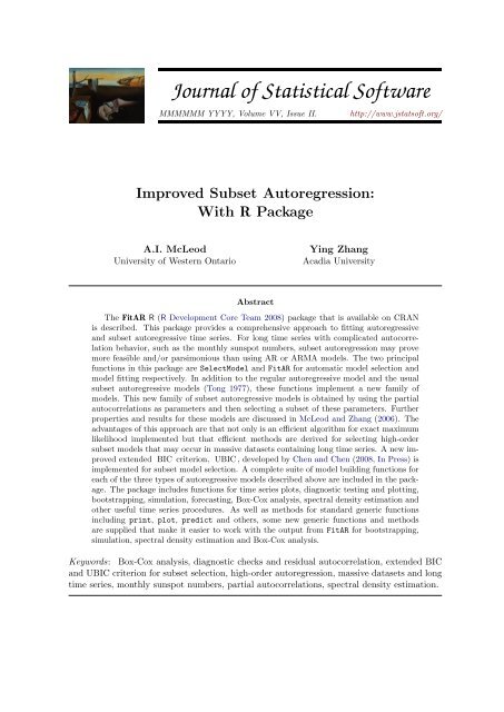
<strong>Improved</strong> <strong>Subset</strong> Autoregression:<br />
<strong>With</strong> R <strong>Package</strong><br />
A.I. McLeod<br />
University of Western Ontario<br />
Ying Zhang<br />
Acadia University<br />
Abstract<br />
The Fit<strong>AR</strong> R (R Development Core Team 2008) package that is available on CRAN<br />
is described. This package provides a comprehensive approach to fitting autoregressive<br />
<strong>and</strong> subset autoregressive time series. For long time series with complicated autocorrelation<br />
behavior, such as the monthly sunspot numbers, subset autoregression may prove<br />
more feasible <strong>and</strong>/or parsimonious than using <strong>AR</strong> or <strong>AR</strong>MA models. The two principal<br />
functions in this package are Select<strong>Model</strong> <strong>and</strong> Fit<strong>AR</strong> for automatic model selection <strong>and</strong><br />
model fitting respectively. In addition to the regular autoregressive model <strong>and</strong> the usual<br />
subset autoregressive models (Tong 1977), these functions implement a new family of<br />
models. This new family of subset autoregressive models is obtained by using the partial<br />
autocorrelations as parameters <strong>and</strong> then selecting a subset of these parameters. Further<br />
properties <strong>and</strong> results for these models are discussed in McLeod <strong>and</strong> Zhang (2006). The<br />
advantages of this approach are that not only is an efficient algorithm for exact maximum<br />
likelihood implemented but that efficient methods are derived for selecting high-order<br />
subset models that may occur in massive datasets containing long time series. A new improved<br />
extended BIC criterion, UBIC , developed by Chen <strong>and</strong> Chen (2008, In Press) is<br />
implemented for subset model selection. A complete suite of model building functions for<br />
each of the three types of autoregressive models described above are included in the package.<br />
The package includes functions for time series plots, diagnostic testing <strong>and</strong> plotting,<br />
bootstrapping, simulation, forecasting, Box-Cox analysis, spectral density estimation <strong>and</strong><br />
other useful time series procedures. As well as methods for st<strong>and</strong>ard generic functions<br />
including print, plot, predict <strong>and</strong> others, some new generic functions <strong>and</strong> methods<br />
are supplied that make it easier to work with the output from Fit<strong>AR</strong> for bootstrapping,<br />
simulation, spectral density estimation <strong>and</strong> Box-Cox analysis.<br />
Keywords: Box-Cox analysis, diagnostic checks <strong>and</strong> residual autocorrelation, extended BIC<br />
<strong>and</strong> UBIC criterion for subset selection, high-order autoregression, massive datasets <strong>and</strong> long<br />
time series, monthly sunspot numbers, partial autocorrelations, spectral density estimation.
2 <strong>Subset</strong> Autoregression<br />
1. Introduction<br />
The family of <strong>AR</strong>(p) models for a time series z t , t = 1, 2, . . . , may be written in operator<br />
notation, φ(B)(z t − µ) = a t , where φ(B) = 1 − φ 1 B − . . . − φ p B p , µ is the mean of the series<br />
<strong>and</strong> a t ∼ NID (0, σ 2 a). It is assumed that the parameters are in the admissible region so that<br />
all roots of the equation φ(B) = 0 lie outside the unit circle. The usual family of subset <strong>AR</strong>(p)<br />
models is obtained by taking a subset of the parameters φ 1 , . . . , φ p , <strong>and</strong> may be written as<br />
φ(B)(z t − µ) = a t , where φ(B) = 1 − φ i1 B − . . . − φ im B im . This family of subset <strong>AR</strong> models<br />
may be denoted by <strong>AR</strong>p(i 1 , . . . , i m ), where 0 ≤ i 1 ≤ i 2 . . . ≤ i m ≤ p 1 .<br />
To define the new family, consider the Durbin-Levinson recursion for the <strong>AR</strong>(p)<br />
φ j,k+1 = φ j,k − φ k+1,k+1 φ k+1−j,k , j = 1, . . . , k, (1)<br />
where k = 1, . . . , p − 1 <strong>and</strong> ζ k+1 = φ k+1,k+1 is the partial autocorrelation at lag k + 1. This<br />
recursion can be used to define a one-to-one, onto, continuous <strong>and</strong> differentiable transformation<br />
(Barndorff-Nielsen <strong>and</strong> Schou 1973; Monahan 1984; Zhang <strong>and</strong> McLeod 2006b, Theorem<br />
1),<br />
(φ 1 , . . . , φ p ) ←→ (ζ 1 , . . . , ζ p ), (2)<br />
where ζ i , i = 1, . . . , p, are the partial autocorrelations at lags 1, . . . , p. The new family of<br />
subset models, denoted by <strong>AR</strong>z(i 1 , . . . , i m ), is obtained by selecting ζ i1 , . . . , ζ im as parameters<br />
<strong>and</strong> constraining other partial autocorrelations as zero 1 . This model forms a subset of the<br />
<strong>AR</strong>(p) model that may be written as φ(B)(z t − µ) = a t , where the parameters φ 1 , . . . , φ p<br />
are reparameterized by eqn. (2). For example, in the <strong>AR</strong>z(1, 3), φ 1 = ζ 1 , φ 2 = −ζ 1 ζ 3 <strong>and</strong><br />
φ 3 = ζ 3 , since ζ 2 = 0. The <strong>AR</strong>p(i 1 , . . . , i m ) <strong>and</strong> <strong>AR</strong>z(i 1 , . . . , i m ) are similar but distinct<br />
models. For example, in the <strong>AR</strong>p(1, 3), ζ 1 = φ 1 /(1 − φ 1 φ 3 − φ 2 3 ), ζ 2 = φ 1 φ 3 /(1 − φ 2 3 ) <strong>and</strong><br />
ζ 3 = φ 3 . The most important advantage of the new parameterization is the efficiency with<br />
which subset <strong>AR</strong> models with large p may be identified. This advantage is important with long<br />
<strong>and</strong> complex time series which are becoming available in massive datasets being collected in<br />
a variety of scientific fields. Asymptotic distributions of the parameter estimates <strong>and</strong> residual<br />
autocorrelations are derived in McLeod <strong>and</strong> Zhang (2006). The notation <strong>and</strong> models are<br />
summarized in Table 1 below.<br />
Abbreviation Description Parameters Lags<br />
<strong>AR</strong>(p) Non-subset <strong>AR</strong> model φ 1 , . . . , φ p 1, . . . , p<br />
<strong>AR</strong>p(i 1 , . . . , i m ) Usual subset <strong>AR</strong> model φ i1 , . . . , φ im i 1 , . . . , i m<br />
<strong>AR</strong>z(i 1 , . . . , i m ) New family of subset <strong>AR</strong> models ζ i1 , . . . , ζ im i 1 , . . . , i m<br />
Table 1: Summary of Families of <strong>AR</strong> <strong>Model</strong>s.<br />
2. <strong>Model</strong> Identification<br />
Table 2 lists the three functions useful in initial model selection.<br />
1 To represent the subset models, the notation <strong>AR</strong>p <strong>and</strong> <strong>AR</strong>z is used in this paper rather than <strong>AR</strong> φ <strong>and</strong><br />
<strong>AR</strong> ζ used in our previous work (McLeod <strong>and</strong> Zhang 2006). This new notation is more convenient in the R<br />
help documentation.
Journal of Statistical Software 3<br />
Function<br />
PacfPlot<br />
Select<strong>Model</strong><br />
TimeSeriesPlot<br />
Purpose<br />
Plot Partial Autocorrelations <strong>and</strong> Limits<br />
Select Best <strong>AR</strong>, <strong>AR</strong>z or <strong>AR</strong>p <strong>Model</strong><br />
Multi-Panel or Single-Panel Time Series Plot with Aspect-Ratio Control<br />
2.1. Time Series Plots<br />
Table 2: <strong>Model</strong> Identification Functions.<br />
Although time series plots can easily be produced with the built-in R function plot or<br />
plot.ts, there are several advantages to using our function TimeSeriesPlot. As pointed<br />
out in Clevel<strong>and</strong> (1993), many stationary time series are best visualized with a relatively<br />
low aspect-ratio <strong>and</strong> it is awkward to do this with st<strong>and</strong>ard R graphics. The function<br />
TimeSeriesPlot adjusts the aspect-ratio using par settings. In the lattice package, the<br />
function xyplot also allows one to control the aspect-ratio. In general, Clevel<strong>and</strong> (1993)<br />
recommends a procedure, banking to 45 o . This algorithm determines the aspect-ratio so as<br />
to make the average slope 45 o . For time series this is only a rough guide since, for stationary<br />
time series, the resulting aspect-ratio will often be too close to zero, <strong>and</strong> for time series<br />
containing strong trends, it makes more sense to bank to the underlying trend. When strong<br />
trends are present, it is usually reasonable to use aspect = 1 but the user should be prepared<br />
to experiment with what aspect-ratio is most effective.<br />
Figure 1 <strong>and</strong> Figure 2 compare the plot.ts <strong>and</strong> TimeSeriesPlot using the built-in lynx time<br />
series. Figure 2 with the lower aspect-ratio shows the asymmetry in the population cycles<br />
more clearly.<br />
When plotting long time series the resolution may be improved by using a multipanel display<br />
which can be easily created using xyplot. Our function TimeSeriesPlot implements a lattice<br />
display for long time series. Figure 3 below illustrates the multipanel time series display for<br />
the Ninemile treering time series.<br />
0 1000 2000 3000 4000 5000 6000 7000<br />
1820 1840 1860 1880 1900 1920<br />
Time<br />
Figure 1:<br />
The lynx series with default aspect-ratio with plot.ts function.
4 <strong>Subset</strong> Autoregression<br />
0 2000 5000<br />
1820 1840 1860 1880 1900 1920<br />
Time<br />
Figure 2: The aspect-ratio in TimeSeriesPlot has been set to 0.25. We can see more clearly<br />
the asymmetry for the lynx series.<br />
Douglas Fir treering series, Nine Mile Canyon, 1194−1964<br />
300<br />
250<br />
200<br />
150<br />
100<br />
50<br />
0<br />
300<br />
250<br />
200<br />
150<br />
100<br />
50<br />
0<br />
600 650 700 750<br />
400 450 500 550 600<br />
200 250 300 350 400<br />
0 50 100 150 200<br />
Observation Number<br />
300<br />
250<br />
200<br />
150<br />
100<br />
50<br />
0<br />
300<br />
250<br />
200<br />
150<br />
100<br />
50<br />
0<br />
Figure 3: Trellis or lattice style graphics are useful for displaying long time series as well as<br />
for choosing a suitable aspect-ratio.<br />
2.2. Partial Autocorrelation Plot<br />
The R function, pacf, plots the usual partial autocorrelations <strong>and</strong> their 95% confidence limits.<br />
Our function PacfPlot 2 is more useful for identifying <strong>AR</strong>z subset models. Given a maximum<br />
order P for the model, the estimated partial autocorrelations ˆζ 1 , . . . , ˆζ P are computed along<br />
2 PacfPlot uses the Burg algorithm as opposed to pacf which uses the Yule-Walker estimates. Many<br />
researchers, for example, Zhang <strong>and</strong> McLeod (2006a) <strong>and</strong> Percival <strong>and</strong> Walden (1993) have found that the<br />
Yule-Walker estimates are not always satisfactory when p ≥ 2 while the least squares method may yield<br />
inadmissible estimates.
Journal of Statistical Software 5<br />
with their estimated st<strong>and</strong>ard errors. The estimated st<strong>and</strong>ard errors are computed from the<br />
large-sample covariance matrix of ˆζ 1 , . . . , ˆζ P given in McLeod <strong>and</strong> Zhang (2006). The plot<br />
produced by PacfPlot shows the 95% confidence interval for each individual of ˆζ i , i = 1, . . . , P .<br />
From this plot, the nonzero subset of partial autocorrelations ζ 1 , . . . , ζ P for the <strong>AR</strong>z model<br />
may be selected.<br />
The use of PacfPlot is illustrated in Figure 4 for the natural logarithms of the built-in lynx<br />
time series. This plot shows that 95% confidence intervals for ˆζ 1 , ˆζ 2 , ˆζ 4 , ˆζ 7 , ˆζ 10 , <strong>and</strong> ˆζ 11 do<br />
not include zero <strong>and</strong> hence the subset partial autocorrelations at lags 1, 2, 4, 7, 10 <strong>and</strong> 11<br />
are significantly different from zero at the 5% level. Thus the <strong>AR</strong>z(1, 2, 4, 7, 10, 11) model is<br />
suggested. Since lags 4 <strong>and</strong> 10 are barely significant at 5%, an <strong>AR</strong>zz(1, 2, 7, 11) model may<br />
also be considered.<br />
pacf<br />
−1.0 −0.5 0.0 0.5 1.0<br />
2 4 6 8 10 12 14<br />
lag<br />
95% confidence intervals for pacf<br />
Figure 4:<br />
Partial autocorrelation plot for identifying an <strong>AR</strong>z model to the lynx time series.<br />
2.3. Automatic <strong>Model</strong> Selection<br />
It is often preferable to use an automatic model selection method. We consider automatic<br />
methods for the non-subset <strong>and</strong> the subset <strong>AR</strong> models. In all model selection algorithms, we<br />
will assume that the mean parameter is included in the model <strong>and</strong> the mean is estimated by<br />
the sample mean.<br />
Non-<strong>Subset</strong> <strong>Model</strong>s<br />
The approximate concentrated log-likelihood for an <strong>AR</strong>(p) model may be written,<br />
( p )<br />
∏<br />
L = −n log (1 − ˆζ k)<br />
2<br />
where n is the series length. When p = 0, L = 0. The AIC model selection criterion,<br />
k=1<br />
(3)<br />
AIC = −2L + 2p (4)
6 <strong>Subset</strong> Autoregression<br />
is evaluated for p = 0, . . . , P , where P is the maximum order 3 . Similarly for the BIC,<br />
BIC = −2L + p log n. (5)<br />
Initially κ 0 c<strong>and</strong>idate models are selected using the AIC/BIC evaluated using the approximate<br />
likelihood in eqn. (3). These models are then refit using exact likelihood method described in<br />
Section 3 <strong>and</strong> new AIC/BIC values are computed. From these models the best κ 1 < κ 0 are<br />
output as the final selection. As noted by Duong (1984) <strong>and</strong> Choi (1992), it is often useful to<br />
consider not just the best model but also close runner-ups. So in this case we would choose<br />
κ 1 > 1. In the function Select<strong>Model</strong>, κ 0 <strong>and</strong> κ 1 correspond to the arguments C<strong>and</strong>idates<br />
<strong>and</strong> Best which have default settings, C<strong>and</strong>idates = 5 <strong>and</strong> Best = 3.<br />
The example below illustrates why this two-step procedure is needed. We consider the highorder<br />
<strong>AR</strong> models fit by Percival <strong>and</strong> Walden (1993, Ch. 10) to the Willamette river data.<br />
Using the Akaike FPE, which is asymptotically equivalent to the AIC (Nishii 1984), Percival<br />
<strong>and</strong> Walden (1993, §10.15) find that the best model is an <strong>AR</strong>(38) which agrees with our<br />
function Select<strong>Model</strong>:<br />
R> Select<strong>Model</strong>(log(Willamette), lag.max = 150, Criterion = "AIC")<br />
p AIC AICx<br />
1 38 -2474.058 -485.9111<br />
2 27 -2473.823 -484.9443<br />
3 39 -2472.308 -485.0843<br />
The AIC-column is based on the exact log-likelihood given in eqn. (8) <strong>and</strong> the AICx-column<br />
is based on the approximate likelihood in eqn. (3). In this case both methods agreed that<br />
the best model was with p = 38 but the exact method selected p = 27 as second best whereas<br />
the approximate method would have selected p = 39.<br />
The default order selection criterion in Select<strong>Model</strong> is BIC since in forecasting applications<br />
this often provides the most suitable model (Koehler <strong>and</strong> Murphree 1988; Davis, Lee, <strong>and</strong><br />
Rodriguez-Yam 2004; Hipel <strong>and</strong> McLeod 1994). For spectral density estimation using nonsubset<br />
models, many authors prefer the AIC (Choi 1992; Percival <strong>and</strong> Walden 1993; Hipel<br />
<strong>and</strong> McLeod 1994).<br />
<strong>Subset</strong> <strong>Model</strong>s<br />
In the case of subset model selection of high-order <strong>AR</strong>, the model space can become very<br />
large. When the model space is large like this, the usual AIC/BIC criteria may select overparameterized<br />
models (Chen <strong>and</strong> Chen 2008, In Press; Broman <strong>and</strong> Speed 2002). Chen<br />
<strong>and</strong> Chen (2008, In Press) have developed the UBIC criterion for this large model space<br />
problem. Therefore, for subset model selection, we have implemented UBIC as the default<br />
in Select<strong>Model</strong> 4 . For comparison, the usual AIC/BIC criteria are also implemented. The<br />
computation of these criteria is outlined next.<br />
3 Akaike (1970, p.216) recommends P = n/10. This is just an empirical rule-of-thumb. In practice, while<br />
P must be taken large enough to obtain an adequate fit, it is important not to take P too large in order to<br />
avoid over-fitting. This is our recommendation for subset models as well.<br />
4 In the non-subset case, our problem is model order selection. In this case, the model space is not large<br />
<strong>and</strong> the UBIC criterion reduces to the usual BIC.
Journal of Statistical Software 7<br />
The approximate concentrated log-likelihood function for an <strong>AR</strong>z(i 1 , . . . , i m ) evaluated at<br />
ˆζ 1 , . . . , ˆζ m may be written (McLeod <strong>and</strong> Zhang 2006, eqn. 15),<br />
⎛<br />
L = −n log ⎝<br />
∏<br />
k∈{i 1 ,...,i m}<br />
⎞<br />
(1 − ˆζ k)<br />
2 ⎠ (6)<br />
where n is the series length. The UBIC criterion (Chen <strong>and</strong> Chen 2008, In Press) may be<br />
written,<br />
(<br />
P<br />
m)<br />
where P is the maximum possible lag.<br />
equivalent ordering of the UBIC.<br />
UBIC = −2L + m log n + 2 log<br />
, (7)<br />
Any value of P such that P ≥ i m produces an<br />
The usual AIC/BIC criteria defined in eqns. (4) <strong>and</strong> (5) may also be used but these criteria<br />
are not recommended for the subset problem. For the model order selection problem in the<br />
non-subset case, the UBIC reduces to the BIC.<br />
The UBIC or AIC/BIC subset can be found simply by ordering the parameters in ascending<br />
order of magnitude, |ˆζ i1 | ≤ |ˆζ i2 | ≤ . . . ≤ |ˆζ iP |, <strong>and</strong> then evaluating successively L starting<br />
with L = 0 for the null model containing only the mean parameter 5 . As in the non-subset<br />
model selection algorithm, a second pass is made after an initial number of c<strong>and</strong>idate models<br />
are found, in which each model is refit using exact maximum likelihood. For the log(lynx)<br />
data, we find using the UBIC,<br />
R> Select<strong>Model</strong>(log(lynx),lag.max = 15, <strong>AR</strong><strong>Model</strong> = "<strong>AR</strong>z", Best = 1)<br />
[1] 1 2 7 10 11<br />
<strong>and</strong> this agrees well with the model suggested by the PacfPlot. To summarize the procedure<br />
used in this example, the best 5 models were found using the approximate likelihood to<br />
estimate the UBIC. Then for each of these 5 models, the exact likelihood was used to determine<br />
the UBIC for each model. Then the best model, the <strong>AR</strong>z(1, 2, 7, 10, 11) was found. For this<br />
data, the model space is not very large <strong>and</strong> consequently, it may be shown that the BIC<br />
selects the <strong>AR</strong>z(1, 2, 7, 10, 11).<br />
<strong>Model</strong> identification for subset <strong>AR</strong>p models is supported using the R subset regression package<br />
leaps. Using this package the best <strong>AR</strong>p subset model is identified using a two-step procedure.<br />
In the first step, the leaps function is used to find the <strong>AR</strong>p(i 1 , . . . , i m ) subsets which when<br />
fit using least squares have minimum residual variance for each i m , m = 0, 1, . . . , P parameters.<br />
For the next step, all P models are refit using our least squares <strong>AR</strong> fitting algorithm,<br />
GetFit<strong>AR</strong>pLS, <strong>and</strong> the exact log-likelihood is determined using Loglikelihood<strong>AR</strong>. Based on<br />
these log-likelihoods, the UBIC/BIC/AIC is re-evaluated <strong>and</strong> the best model is selected.<br />
As shown below, the model selected by Tong (1977) for the lynx series, <strong>AR</strong>p(1, 2, 4, 10, 11),<br />
is selected using Select<strong>Model</strong>,<br />
R> Select<strong>Model</strong>(log(lynx),lag.max=15,<strong>AR</strong><strong>Model</strong>="<strong>AR</strong>p",Criterion="BIC",Best=1)<br />
5 As in PacfPlot, the Burg estimates are used for the partial autocorrelations.
8 <strong>Subset</strong> Autoregression<br />
[1] 1 2 4 10 11<br />
however, the UBIC selects the more parsimonious <strong>AR</strong>p(1, 2, 9, 12). When Best > 1, the<br />
output from Select<strong>Model</strong> is a list <strong>and</strong> is defined as a "Selectmodel" S3 class object. This<br />
output may be graphically viewed using the plot function. For the lynx dataset, Figure 5<br />
compares the 3 best <strong>AR</strong>p <strong>and</strong> <strong>AR</strong>z subset models selected using the UBIC <strong>and</strong> BIC. In<br />
Figure 5, the left vertical axis shows the scale in terms of BIC while the right one uses<br />
relative plausibility, defined by exp{( BIC 1 − BIC 0 )/2}, where BIC 0 <strong>and</strong> BIC 1 denote the<br />
BIC values for the best model <strong>and</strong> the alternative respectively. Likelihood <strong>and</strong> plausibility<br />
for time series models were introduced by Akaike (1978) <strong>and</strong> Akaike (1979). As with the<br />
relative likelihood (Fisher 1959; Royall 1997; Sprott 2000), alternative models with relative<br />
plausibility less than 1% may be said to be implausible. As shown in Figure 5, the BIC <strong>and</strong><br />
UBIC select the same best three <strong>AR</strong>z models although for the <strong>AR</strong>p a more parsimonious<br />
model is selected using the UBIC than with the BIC.<br />
<strong>AR</strong>p model selection<br />
<strong>AR</strong>p model selection<br />
BIC<br />
−150.5 −149.5 −148.5 −147.5<br />
2 4 6 8 10 12<br />
1 0.573 0.241<br />
Relative Plausibility<br />
UBIC<br />
−132 −131 −130 −129<br />
2 4 6 8 10 12<br />
1 0.161<br />
Relative Plausibility<br />
lags<br />
lags<br />
<strong>AR</strong>z model selection<br />
<strong>AR</strong>z model selection<br />
BIC<br />
−144.5 −143.5 −142.5<br />
2 4 6 8 10<br />
1 0.721 0.357<br />
Relative Plausibility<br />
UBIC<br />
−126.5 −125.5 −124.5 −123.5<br />
2 4 6 8 10<br />
1 0.504 0.222<br />
Relative Plausibility<br />
lags<br />
lags<br />
Figure 5: Plot of the output from Select<strong>Model</strong> with Best = 3 for <strong>AR</strong>p <strong>and</strong> <strong>AR</strong>z models<br />
using BIC <strong>and</strong> UBIC for subset selection for the logged lynx series.<br />
The best subset for <strong>AR</strong>z models is easily found even when P is large since only sorting is<br />
needed. On the other h<strong>and</strong>, for the <strong>AR</strong>p best subset selection, the leaps package, available
Journal of Statistical Software 9<br />
on CRAN, is used <strong>and</strong> this package implements an exponential-time branch-<strong>and</strong>-bound algorithm.<br />
The function used, leaps, is interfaced to Fortran for maximum efficiency. But<br />
still it is limited to a maximum order of around P = 50 or so due to the rapidly increasing<br />
computing time needed as P increases. Thus it is possible to fit much higher order subset<br />
models using the <strong>AR</strong>z model. This is illustrated with the Zurich monthly sunspots 1749−1983<br />
available in R as a built-in dataset, sunspots. Taking a maximum model order of P = 200<br />
<strong>and</strong> using a square-root transformation, the best non-subset <strong>AR</strong> <strong>and</strong> subset <strong>AR</strong>z models were<br />
determined. In the case of <strong>AR</strong> model selection the <strong>AR</strong>(27) <strong>and</strong> <strong>AR</strong>(21) models were selected<br />
using the AIC <strong>and</strong> BIC criteria. For the subset selection, AIC, BIC <strong>and</strong> UBIC were used <strong>and</strong><br />
the number of parameters not including the mean in the selected models were 55, 18 <strong>and</strong> 8<br />
respectively for AIC, BIC <strong>and</strong> UBIC. Figure 6 compares the spectral density functions for the<br />
estimated models. The AIC subset model spectral density was very jagged <strong>and</strong> is not shown<br />
in Figure 6 6 .<br />
AIC Order Selection<br />
BIC <strong>Subset</strong> Selection<br />
Log Sdf<br />
0 2 4 6<br />
0.0 0.5 1.0 1.5<br />
frequency<br />
<strong>AR</strong>(27)<br />
BIC Order Selection<br />
0.0 0.5 1.0 1.5<br />
Log Sdf<br />
−1 0 1 2 3 4 5 6<br />
Log Sdf<br />
0 2 4 6<br />
frequency<br />
<strong>AR</strong>z(1,2,3,4,5,10,11,13,15,16,17,18,20,21,24,67,70,92)<br />
UBIC <strong>Subset</strong> Selection<br />
Log Sdf<br />
−1 0 1 2 3 4 5 6<br />
0.0 0.5 1.0 1.5<br />
frequency<br />
<strong>AR</strong>(21)<br />
0.0 0.5 1.0 1.5<br />
frequency<br />
<strong>AR</strong>z(1,2,3,4,5,11,16,18)<br />
Figure 6: Logged spectral density functions of the non-subset <strong>AR</strong> <strong>and</strong> subset <strong>AR</strong>z models<br />
fitted to the square-root of the sunspots series.<br />
6 See Example 3 in the documentation for sdfplot for an R script to estimate the spectral density function<br />
for the monthly sunspot series by using the AIC criterion to fit an <strong>AR</strong>z model.
10 <strong>Subset</strong> Autoregression<br />
3. Estimation<br />
The log-likelihood function given n time series observations z 1 , . . . , z n from a covariance stationary<br />
Gaussian time series with mean µ <strong>and</strong> autocovariance function γ k , k = 0, 1, . . ., may<br />
be determined from the multivariate normal distribution. Letting M n = Γ n /σ 2 a where Γ n is<br />
the covariance matrix of n successive observations <strong>and</strong> maximizing the log-likelihood function<br />
over σ 2 a, the concentrated log-likelihood may be written, after dropping constants,<br />
L(φ) = − n 2 log(S(φ)/n) − 1 2 log(g n), (8)<br />
where S(φ) = z ′ Mn<br />
−1 z, g n = det(M n ) <strong>and</strong> ˆσ a 2 = S(φ)/n where φ = (φ 1 , . . . , φ p ). Note that L<br />
given in eqn. (6) is an affine large-sample approximation to the exact log-likelihood given in<br />
eqn. (8).<br />
Assuming that the mean is known, the exact log-likelihood function may be computed in O(1)<br />
flops independent of n in repeated function evaluations after an initial setup computation is<br />
performed (McLeod <strong>and</strong> Zhang 2006, §2.1). This is done by conditioning on the sufficient<br />
statistics, D i,j = z i z j + · · · + z n−j z n−i , where we have assumed a mean-zero time series. The<br />
R function optim is then used to maximize the log-likelihood function. Initial starting values<br />
are obtained using Burg estimates. This exact maximum likelihood estimation algorithm is<br />
implemented in our functions Fit<strong>AR</strong> <strong>and</strong> Get<strong>AR</strong>Fit. The function Get<strong>AR</strong>Fit may be preferred<br />
for bootstrapping applications while Fit<strong>AR</strong> is intended as the main function for model fitting<br />
when diagnostic checking <strong>and</strong> forecasting are important.<br />
Fit<strong>AR</strong> also computes the covariance matrix of the estimates, residuals, fitted values <strong>and</strong> some<br />
diagnostic checks. The function Fit<strong>AR</strong> returns a S3 class object "Fit<strong>AR</strong>". Generic functions<br />
print, summary, coef, resid, <strong>and</strong> plot are supplied. In addition some new generic functions<br />
Boot <strong>and</strong> sdfplot are defined <strong>and</strong> methods are given for class "Fit<strong>AR</strong>", "ts" <strong>and</strong> other<br />
objects of interest. More methods are supplied for these functions in McLeod, Yu, <strong>and</strong> Zinovi<br />
(2008).<br />
Fit<strong>AR</strong> <strong>and</strong> getFit<strong>AR</strong> use several other functions which may be of interest in some applications<br />
<strong>and</strong> are described briefly in Appendix A. In Appendix B, we discuss the perils of fitting the<br />
<strong>AR</strong>p model using exact MLE. This provides another reason for preferring the <strong>AR</strong>z model.<br />
3.1. Exact MLE for Mean<br />
Assuming that (φ 1 , . . . , φ p ) are known, the exact MLE for mean µ is given by<br />
ˆµ = 1′ nΓ −1<br />
n z<br />
1 ′ nΓ −1 , (9)<br />
n 1 n<br />
where 1 n denotes the n dimensional column vector with all entries equal to 1, z = (z 1 , . . . , z n )<br />
<strong>and</strong> Γ −1<br />
n denotes the inverse of the covariance matrix of n successive observations. Since<br />
ˆµ does not depend on σa, 2 we may assume without loss of generality that σa 2 = 1. Direct<br />
evaluation of eqn. (9) using the exact inverse matrix derived by Siddiqui (1958) would require<br />
O(n 2 ) flops. A more efficient algorithm is given in McLeod <strong>and</strong> Zhang (2008) for evaluating<br />
eqn. (9) in O(n) flops <strong>and</strong> this is implemented in our R function Get<strong>AR</strong>MeanMLE. As a check<br />
for the correctness of Get<strong>AR</strong>MeanMLE, in the example section of the help documentation for<br />
Get<strong>AR</strong>MeanMLE, we provide a R script which compares the results obtained by computing the<br />
MLE of the mean µ directly <strong>and</strong> using Get<strong>AR</strong>MeanMLE.
Journal of Statistical Software 11<br />
When (φ 1 , . . . , φ p ) is unknown, the iterative algorithm given in McLeod <strong>and</strong> Zhang (2008, §2.2)<br />
may be used to obtain the simultaneous joint MLEs of µ <strong>and</strong> the other model parameters.<br />
This iterative algorithm is implemented in Fit<strong>AR</strong> with the option MeanMLEQ = TRUE. In the<br />
documentation for Fit<strong>AR</strong>, an example is given to demonstrate the agreement with results<br />
obtained by the built-in function arima.<br />
Some simulations were carried out to compare the timings for GetFit<strong>AR</strong>, Fit<strong>AR</strong> <strong>and</strong> the builtin<br />
function ar for fitting nonsubset <strong>AR</strong>(p), p = 1, 2 <strong>and</strong> p = 20, 40 7 . The main purpose of<br />
these timings is just to indicate the relative computer times for the three different algorithms.<br />
As far as accuracy is concerned, there is no meaningful difference in accuracy between Fit<strong>AR</strong><br />
<strong>and</strong> ar when the latter function converges. As noted below, ar does not always work <strong>and</strong><br />
sometimes it fails completely. It seems reasonable to recommend that users avoid the exact<br />
MLE option in ar. Between GetFit<strong>AR</strong> <strong>and</strong> Fit<strong>AR</strong> there are some slight differences in the<br />
estimates but overall there does not seem to be any notable difference in accuracy for the<br />
models in this experiment.<br />
For each model, the admissible parameters were r<strong>and</strong>omly selected by r<strong>and</strong>omly selecting<br />
partial autocorrelations uniformly from −1 to 1 <strong>and</strong> then reparameterizing through eqn. (2).<br />
Various lengths of series were used from n = 50, 100, 200, 500, 1000. Since the timings do not<br />
vary much once n <strong>and</strong> p are fixed, only ten simulations were done for each of these parameter<br />
settings. At least ten are needed because for the low order <strong>AR</strong> models with small n the timing<br />
for a single fitting is too short to get an accurate value. The average CPU times required for<br />
simulations <strong>and</strong> fitting are given below in Table 3. During fitting, ar reported one error in<br />
optim which is shown below:<br />
Error in optim(init[mask], arma0f, method = "BFGS", hessian = TRUE,<br />
control = optim.control): non-finite finite-difference value [3]<br />
This error was trapped using the built-in R function try. Many warning messages about convergence<br />
were also generated by ar. On the other h<strong>and</strong> GetFit<strong>AR</strong> or Fit<strong>AR</strong> worked correctly<br />
in all cases without generating any messages. The experiment was repeated, this time with<br />
p = 20, 40 <strong>and</strong> n = 1000, 2000, 5000. Once again ar generated error <strong>and</strong> warning messages.<br />
<strong>With</strong> GetFit<strong>AR</strong>, the sample mean was used but for Fit<strong>AR</strong> the iterative algorithm was used to<br />
compute the exact MLE for the mean as well as the other parameters. <strong>With</strong> ar the option<br />
method="mle" was used. All timings reported in this paper are for a Pentium 4 processor<br />
at 3 GHz PC running Windows XP with 2 GB RAM. The CPU times in Table 3 show that<br />
Fit<strong>AR</strong> is much faster than ar for p = 40. If the sample mean is used then GetFit<strong>AR</strong> is always<br />
very fast <strong>and</strong> for most <strong>AR</strong> models that seem to occur in practice, there is not much difference<br />
between using the sample mean <strong>and</strong> the exact MLE.<br />
7 The R script for doing these computations is provided at http://www.stats.uwo.ca/faculty/aim/2007/<br />
Fit<strong>AR</strong>/
12 <strong>Subset</strong> Autoregression<br />
n GetFit<strong>AR</strong> Fit<strong>AR</strong> ar GetFit<strong>AR</strong> Fit<strong>AR</strong> ar<br />
<strong>AR</strong>(1)<br />
<strong>AR</strong>(2)<br />
50 0.01 0.02 0.02 0.02 0.08 0.03<br />
100 0.01 0.03 0.03 0.02 0.08 0.03<br />
200 0.02 0.05 0.04 0.03 0.10 0.04<br />
500 0.04 0.09 0.06 0.05 0.14 0.07<br />
1000 0.07 0.15 0.09 0.09 0.21 0.11<br />
<strong>AR</strong>(20)<br />
<strong>AR</strong>(40)<br />
1000 0.14 5.52 2.04 0.24 34.66 47.60<br />
2000 0.20 5.52 1.98 0.34 22.99 51.60<br />
5000 0.37 5.89 2.60 0.60 24.09 44.85<br />
Table 3: Timings for GetFit<strong>AR</strong>, Fit<strong>AR</strong> <strong>and</strong> ar. For each n <strong>and</strong> each p, 100 series were<br />
simulated <strong>and</strong> the models estimated using the functions GetFit<strong>AR</strong>, Fit<strong>AR</strong> <strong>and</strong> ar. The average<br />
time over all 100 simulations is reported for each parameter combination. These timings are<br />
illustrative of the relative performance of the functions but are highly system dependent. A<br />
3.6 GHz Pentium PC with R Version 2.70 running Windows XP was used.<br />
3.2. Box-Cox Analysis<br />
Box <strong>and</strong> Cox (1964) derived a maximum likelihood method for estimating the transformation<br />
parameter λ in the family of transformations,<br />
{<br />
z (λ) (z<br />
λ<br />
t = t − 1)/λ λ ≠ 0<br />
log(z t ) λ = 0<br />
for data z t , t = 1, . . . , n, from a normal linear regression <strong>and</strong> ANOVA. This method was<br />
adapted to <strong>AR</strong>IMA time series in Hipel <strong>and</strong> McLeod (1977, eqn. 10, p.571). For autoregressive<br />
models, the concentrated loglikelihood function can be written,<br />
L(φ, λ) = − n 2 log(S(φ)/n) − 1 n∑<br />
2 log(g n) + (1 − λ) log(z t ). (10)<br />
t=1<br />
For fixed λ we can maximize over φ to obtain L(λ). The function L(λ) may be maximized<br />
numerically with the optimize function to obtain the MLE, ˆλ. It is convenient to plot the<br />
relative likelihood function R(λ) = L(λ)/L(ˆλ). The relative likelihood, R(λ), itself provides<br />
a quantification of the relative plausibility of various values of λ (Sprott 2000, §2.4 <strong>and</strong> §4.5).<br />
It may be shown that a 95% confidence interval based on the likelihood-ratio test corresponds<br />
to R(λ) ≥ 0.1465. A horizonal line is drawn to indicate a 95% confidence interval for λ.<br />
The function BoxCox is implemented as a generic function with methods for classes "Fit<strong>AR</strong>",<br />
"Arima", "ts" <strong>and</strong> "numeric". BoxCox.Fit<strong>AR</strong> parses its input to construct the likelihood<br />
function in eqn. (10) <strong>and</strong> then the MLE is determined using optimize. A plot of the likelihood<br />
function is determined to show all values of λ with plausibility greater than 1% as well as a<br />
horizontal line indicating the 95% confidence interval. In Figure 7, we compare the Box-Cox<br />
analysis for the lynx time series using our function <strong>and</strong> the boxcox function in the R library
Journal of Statistical Software 13<br />
Relative Likelihood Analysis<br />
95% Confidence Interval<br />
R(λ)<br />
0.0 0.2 0.4 0.6 0.8 1.0<br />
λ^ = 0.073<br />
−0.1 0.0 0.1 0.2<br />
λ<br />
log−Likelihood<br />
−892 −888 −884<br />
95%<br />
0.0 0.1 0.2 0.3 0.4 0.5 0.6<br />
λ<br />
Figure 7: Top graph shows output from BoxCox.Fit<strong>AR</strong> <strong>and</strong> bottom graph from boxcox for<br />
fitting <strong>AR</strong>p(1, 2, 4, 10, 11) to lynx series.<br />
Relative Likelihood Analysis<br />
95% Confidence Interval<br />
R(λ)<br />
0.0 0.2 0.4 0.6 0.8 1.0<br />
λ^ = 0.051<br />
−0.4 −0.2 0.0 0.2 0.4<br />
λ<br />
Figure 8:<br />
Box-Cox analysis produced by BoxCox(AirPassengers).<br />
MASS. For the lynx time series we fit the <strong>AR</strong>p(1, 2, 4, 10, 11) model by least-squares using<br />
Fit<strong>AR</strong>p. In this case, the output from Fit<strong>AR</strong>p contains the design matrix for the regression<br />
as well as the column for the dependent variable. These results were then used with the<br />
MASS boxcox function to obtain the bottom plot in Figure 7. The difference in the plots is
14 <strong>Subset</strong> Autoregression<br />
Relative Likelihood Analysis<br />
95% Confidence Interval<br />
R(λ)<br />
0.0 0.2 0.4 0.6 0.8 1.0<br />
λ^ = −0.552<br />
−1.0 −0.8 −0.6 −0.4 −0.2<br />
λ<br />
Figure 9:<br />
Box-Cox analysis produced by BoxCox(rivers).<br />
substantial. The top plot using BoxCox.Fit<strong>AR</strong> shows that a log transformation is reasonable<br />
choice whereas the bottom plot strongly suggests otherwise <strong>and</strong> favors a transformation such<br />
as a cube-root. The reason for the difference is that in BoxCox.Fit<strong>AR</strong> the log-likelihood in<br />
eqn. (10) is used whereas in boxcox the approximate log-likelihood corresponding to linear<br />
regression is used.<br />
Annual tobacco production, U.S., 1871−1984<br />
Lbs., millons<br />
500 1000 1500 2000<br />
1880 1900 1920 1940 1960 1980<br />
Time<br />
Figure 10:<br />
Time series plot for annual Tobacco production series.<br />
BoxCox.ts <strong>and</strong> BoxCox.numeric enable one to do a Box-Cox analysis for arbitrary time series
Journal of Statistical Software 15<br />
Relative Likelihood Analysis<br />
95% Confidence Interval<br />
R(λ)<br />
0.0 0.2 0.4 0.6 0.8 1.0<br />
λ^ = 0.423<br />
0.0 0.2 0.4 0.6 0.8<br />
λ<br />
Tobacco production,US, 1871−1984<br />
Figure 11:<br />
Box-Cox analysis for annual tobacco production series.<br />
as well as simple r<strong>and</strong>om samples. <strong>With</strong> BoxCox.ts, the untransformed data is fit by a highorder<br />
<strong>AR</strong>(p) model which is then used for Box-Cox analysis. In practice, this procedure<br />
often works well even for non-stationary time series as is shown in Figure 8 for the R dataset<br />
AirlinePassengers. An example of using BoxCox.numeric for the R built-in rivers data<br />
set is shown in Figure 9.<br />
The function BoxCox.Arima implements a Box-Cox analysis for time series fit with the R<br />
arima function. An illustrative example is provided by the time series of annual production<br />
of Tobacco in the U.S. for the period 1871-1984 (See Figure 10). Note the increase in variability.<br />
Since this variability is related to level, a model of the Box-Cox transformed series<br />
provides a much simpler alternative to the more complex <strong>AR</strong>IMA-G<strong>AR</strong>CH approach (Wei<br />
2005, p.379). Wei (2005, p.120) also suggested an <strong>AR</strong>IMA(0, 1, 1) to the logarithms of this<br />
series. However Box-Cox analysis indicates that a square-root transformation works much<br />
better than logarithms (Figure 11).<br />
4. Diagnostic Checks<br />
A methods function plot.Fit<strong>AR</strong> is supplied so that the generic function plot can be used<br />
for a variety of diagnostic plots for Fit<strong>AR</strong> class objects. The default is with option terse =<br />
TRUE which produces a plot of the p-values of the Ljung-Box portmanteau test (Ljung <strong>and</strong><br />
Box 1978) <strong>and</strong> a plot of the residual autocorrelations with simultaneous 95% limits (Hosking<br />
<strong>and</strong> Ravishanker 1993). Both these plots appear as a panel display. These are usually the<br />
most important diagnostics. The default diagnostic plots shown in Figure 12 are produced<br />
by:<br />
R> ans
16 <strong>Subset</strong> Autoregression<br />
R> plot(ans)<br />
Ljung−Box Test<br />
p−value<br />
0.0 0.2 0.4 0.6 0.8 1.0<br />
10 15 20 25<br />
lag<br />
Residual autocorrelation: <strong>AR</strong>p(1,2,4,10,11)<br />
Simultaneous 95% Interval<br />
−0.3 −0.1 0.1 0.2 0.3<br />
0 5 10 15 20 25 30<br />
lag<br />
Figure 12:<br />
lynx series.<br />
Basic diagnostic plots for <strong>AR</strong>p(1, 2, 4, 10, 11) model fit to the logarithm of the<br />
When terse = FALSE, after the plots shown in Figure 12, seven more plots are produced in<br />
the order as follows:<br />
• Normal probability plot <strong>and</strong> the p-value for an ominbus normality test of the Jarque-<br />
Bera test (Jarque <strong>and</strong> Bera 1987). This is useful in detecting outliers or thick tails.<br />
Thick tails are a characteristic of <strong>AR</strong>CH/G<strong>AR</strong>CH models (Tsay 2005, Ch. 3) so this<br />
test may suggest that some form of conditional heteroscedasticity is present.<br />
• Box-<strong>and</strong>-whisker plot of the residuals. This is useful in detecting skewness. Skewness<br />
may indicate a power transformation. On the other h<strong>and</strong>, if the residuals are<br />
symmetric but outliers are present, some form of conditional heteroscedasticity may be<br />
present. Various types of <strong>AR</strong>CH/G<strong>AR</strong>CH models may be used for modeling conditional<br />
heteroscedasticity. A freely available <strong>and</strong> good quality Windows XP software package<br />
JMulti can be used for this type of modeling (Herwartz 2004).
Journal of Statistical Software 17<br />
• Plots of the time series <strong>and</strong> a bootstrap version of the time series. This gives some idea<br />
of whether or not important features in the time series appear in the simulated model.<br />
• Monotone spread plot (Clevel<strong>and</strong> 1979, 1993). This type of residual diagnostic plot is<br />
useful for detecting situations where the variance depends on the level or mean. In<br />
general Clevel<strong>and</strong> (1993) suggested plotting the square root of the absolute residual vs.<br />
the fitted value <strong>and</strong> then visualizing the relationship using a suitable loess smooth. The<br />
R function lowess with f = 1 is used. For time series models, the fitted value represents<br />
a conditional mean. If the model is adequate, the loess curve should be approximately<br />
horizontal. If it is monotonic up or down, a power transformation could be used to<br />
remove this dependence.<br />
• Residual-fit spread (RFS) plot (Clevel<strong>and</strong> 1993). This plot is useful for visualizing how<br />
much of the variation in the data is explained by model <strong>and</strong> so whether the model may<br />
be useful for forecasting. Alternatively, the coefficient of determination, R 2 , defined as<br />
the ratio of the variance of the one-step forecast divided by the series variance may be<br />
used. For the lynx <strong>and</strong> <strong>AR</strong>p(1, 2, 7, 10, 11), R 2 = 85%, as shown below,<br />
R> z var(fitted(Fit<strong>AR</strong>p(z,c(1,2,7,10,11))))/var(z)<br />
[1] 0.8536185<br />
The RFS plot is shown in Figure 13.<br />
• Plots of the observed autocorrelation function, the fitted theoretical autocorrelation<br />
function <strong>and</strong> the sample autocorrelation of a parametric bootstrap. In many cases a<br />
good model can be expected to match the main features of the sample autocorrelations,<br />
particularly at the lower lags. However, caution is necessary since it is well known<br />
that the sample autocorrelations may be highly autocorrelated with large variances<br />
(Box, Jenkins, <strong>and</strong> Reinsel 1994, §2.1.6). In some cases, such as highly autocorrelated<br />
fractional noise, the sample autocorrelations may have very large biases (Newbold <strong>and</strong><br />
Agiakloglou 1993). In this situation, even when the model has been correctly specified<br />
<strong>and</strong> fit, the sample autocorrelations may not resemble very well the theoretical autocorrelations.<br />
This is quite a surprising, but in hindsight, not an unreasonable result. To<br />
the degree that fractional noise may be approximated by a high-order <strong>AR</strong> model, this<br />
problem can be expected to occur with some <strong>AR</strong> models as well. In summary, we can<br />
say that it may happen that even for a correctly fit model, the sample <strong>and</strong> theoretical<br />
autocorrelations might not match very well <strong>and</strong> there may be more similarity in the<br />
sample autocorrelations of the data <strong>and</strong> the bootstrap version.<br />
• Plot of the fitted spectral density function.<br />
summary of the model.<br />
This plot provides a frequency domain<br />
Because of the large number of graphics windows, the default behavior of plot is to delete all<br />
graphics windows before producing the plots. This default can be bypassed by using the optional<br />
argument clearGraphics = FALSE. Some of the diagnostic checks are also available as<br />
separate functions as shown in Table 4. For more details, please see the online documentation.
18 <strong>Subset</strong> Autoregression<br />
0.0 0.2 0.4 0.6 0.8 1.0<br />
Fitted Values minus Mean<br />
Residuals<br />
2<br />
1<br />
0<br />
−1<br />
−2<br />
0.0 0.2 0.4 0.6 0.8 1.0<br />
f−value<br />
Figure 13: RFS plot for <strong>AR</strong>p(1, 2, 4, 10, 11) model fit to the logarithm of the lynx series. For<br />
this model, R 2 = 85%.<br />
Function<br />
Boot<br />
Boot.Fit<strong>AR</strong><br />
Boot.ts<br />
LjungBoxTest<br />
LBQPlot<br />
RacfPlot<br />
JarqueBeraTest<br />
Purpose<br />
Generic Bootstrap Function<br />
Simulate a Fitted <strong>AR</strong><br />
Parametric Time Series Bootstrap<br />
Ljung-Box Test for R<strong>and</strong>omness<br />
Plot Ljung-Box Test P-value vs Lag<br />
Residual Autocorrelation Plot<br />
Jarque-Bera Normality Test<br />
Table 4: <strong>Model</strong> Diagnostic Checking Functions.<br />
5. Other Useful Time Series Functions<br />
We give a brief overview of the functions shown in Table 5. For more details <strong>and</strong> examples,<br />
please see the online R documentation.<br />
5.1. AcfPlot: Correlation Plots<br />
The function AcfPlot is useful for plotting other types of correlation functions, for example,<br />
the residual autocorrelations or the inverse autocorrelations. Clevel<strong>and</strong> (1971) used the inverse<br />
autocorrelations to select an <strong>AR</strong>p(1, 2, 7) model for the Series A time series. The example
Journal of Statistical Software 19<br />
Function<br />
AcfPlot<br />
<strong>AR</strong>1Est<br />
<strong>AR</strong>Sdf<br />
<strong>AR</strong>ToMA<br />
<strong>AR</strong>ToPacf<br />
cts<br />
BackcastResiduals<strong>AR</strong><br />
InformationMatrix<strong>AR</strong><br />
InformationMatrix<strong>AR</strong>p<br />
InformationMatrix<strong>AR</strong>z<br />
InvertibleQ<br />
PacfDL<br />
PacfTo<strong>AR</strong><br />
Plot<strong>AR</strong>Sdf<br />
sdfplot<br />
sdfplot.Fit<strong>AR</strong><br />
sdfplot.Arima<br />
sdfplot.ar<br />
sdfplot.ts<br />
sdfplot.numeric<br />
SimulateGaussian<strong>AR</strong><br />
Readts<br />
Tacvf<strong>AR</strong><br />
TacvfMA<br />
VarianceRacf<strong>AR</strong><br />
VarianceRacf<strong>AR</strong>p<br />
VarianceRacf<strong>AR</strong>z<br />
Purpose<br />
Basic ACF Plotting<br />
Exact MLE for <strong>AR</strong>(1)<br />
Autoregressive Spectral Density Function<br />
Coefficients in Infinite Moving Average Expansion<br />
Reparametrize <strong>AR</strong> Coefficients in Terms of PACF<br />
Concantenate Time Series<br />
Innovation Residuals in <strong>AR</strong><br />
Information Matrix for <strong>AR</strong>(p)<br />
Fisher Information Matrix <strong>Subset</strong> Case, <strong>AR</strong>p<br />
Fisher Information Matrix <strong>Subset</strong> Case, <strong>AR</strong>z<br />
Test if Invertible or Stationary-casual<br />
Partial Autocorrelations via Durbin-Levinson<br />
Transform from PACF Parameters to <strong>AR</strong> Coefficients<br />
Plot <strong>AR</strong> or <strong>AR</strong>MA Spectral Density<br />
Autoregressive Spectral Density Estimation<br />
Autoregressive Spectral Density Estimation for “Fit<strong>AR</strong>”<br />
Spectral Density of Fitted <strong>AR</strong>IMA <strong>Model</strong><br />
Spectral Density of Fitted <strong>AR</strong>IMA <strong>Model</strong><br />
Autoregressive Spectral Density Estimation for “ts” Object<br />
Autoregressive Spectral Density Estimation for “numeric”<br />
Autoregression Simulation<br />
Input a Time Series<br />
Theoretical Autocovariance Function of <strong>AR</strong><br />
Theoretical Autocovariances for Moving Average Process<br />
Covariance Matrix Residual Autocorrelations for <strong>AR</strong><br />
Covariance Matrix Residual Autocorrelations for <strong>AR</strong>p<br />
Covariance Matrix Residual Autocorrelations for <strong>AR</strong>z<br />
Table 5: Other Useful Time Series Functions.<br />
given in the online help documentation for AcfPlot shows how to compute <strong>and</strong> plot the<br />
inverse autocorrelations.<br />
5.2. <strong>AR</strong>1Est: Exact MLE for <strong>AR</strong>(1)<br />
The function <strong>AR</strong>1Est evaluates the exact MLE for a mean-zero <strong>AR</strong>(1) model using a closed<br />
form solution (Zhang 2002). This function is useful in bootstrapping <strong>and</strong> Monte-Carlo since<br />
it is fast, accurate <strong>and</strong> reliable.<br />
5.3. <strong>AR</strong>Sdf <strong>and</strong> Plot<strong>AR</strong>Sdf: Autoregressive Spectral Density<br />
The Fast Fourier Transform is used to evaluate the <strong>AR</strong> spectral density function,
20 <strong>Subset</strong> Autoregression<br />
f(λ) = 1 σa<br />
2<br />
2π |φ(e −2πiλ )| 2 (11)<br />
at a large number of equally spaced frequencies in the range (0, π). By default 2 8 = 256<br />
equally spaced frequencies, λ j = 0.5πj/256, j = 1, . . . , 256. The function <strong>AR</strong>Sdf produces the<br />
vector output (f(λ 1 ), . . . , f(λ 256 )) taking σ 2 a = 1 in eqn. (11).<br />
5.4. <strong>AR</strong>ToMA: Moving-average Approximation<br />
This function is used in computing the variances of the residual autocorrelations <strong>and</strong> in<br />
constructing plots of the residual autocorrelations. This type of computation arises also in<br />
other computations such as in the confidence limits for forecasts from <strong>AR</strong> models.<br />
5.5. <strong>AR</strong>ToPacf <strong>and</strong> PacfTo<strong>AR</strong>: Reparameterization<br />
These functions are central to working with <strong>AR</strong>z models. For many purposes it is necessary<br />
to convert from one parameterization to the other.<br />
5.6. BackcastResiduals<strong>AR</strong>: Compute Residuals<br />
The innovation residuals for a fitted <strong>AR</strong>(p) may be computed recursively from<br />
â t = (z t − ˆµ) − φ 1 (z t−1 − ˆµ) − . . . − φ p (z t−p − ˆµ), (12)<br />
for t = p + 1, . . . , n. For t = 1, . . . , p, the conditional expected value of a t may be computed<br />
by backforecasting the z t for t = 0, −1, − . . . , Q for Q large enough so that the backforecast<br />
value of z t is approximately µ for all t ≤ Q. Then the required residuals may be computed<br />
directly using eqn. (12). This backcasting approach is described in detail in Box et al. (1994,<br />
§6.4.3).<br />
5.7. Concatenation of Time Series<br />
The function cts allows values to be easily concatenated to an existing time series object.<br />
See documentation for more details.<br />
5.8. Information Matrix<br />
The large-sample Fisher information per observation can be obtained for <strong>AR</strong>, <strong>AR</strong>p <strong>and</strong> <strong>AR</strong>z<br />
models. This is used in Fit<strong>AR</strong> to obtain the estimated st<strong>and</strong>ard errors of the estimated<br />
parameters. St<strong>and</strong>ard errors can also be obtained by using the observed Fisher information<br />
that is obtained by numerically differentiating the log-likelihood function. Our preference is to<br />
use the theoretical information matrix since it is well-known that numerical differentiation may<br />
be unreliable (Fröberg 1969, Ch.9, p.192). We have found for simulations <strong>and</strong> bootstrapping<br />
applications this unreliability does occasionally arise resulting in negative variances <strong>and</strong> other<br />
difficulties. St<strong>and</strong>ard errors may also be estimated by bootstrapping (Box <strong>and</strong> Luceño 1997).<br />
Table 6 below compares the bootstrap estimates with the large-sample ones. The script to<br />
generate these results is included in the online documentation for Boot.Fit<strong>AR</strong>. It took about<br />
18 seconds for the 100 bootstrap replications used in Table 6.
Journal of Statistical Software 21<br />
Estimate Bootstrap Large-Sample<br />
ˆζ 1 0.024 0.018<br />
ˆζ 2 0.095 0.086<br />
ˆζ 4 0.069 0.063<br />
ˆζ 7 0.112 0.099<br />
ˆζ 10 0.113 0.089<br />
ˆζ 11 0.091 0.088<br />
Table 6: Comparison of Bootstrap <strong>and</strong> Large-Sample Estimates of the St<strong>and</strong>ard Deviations<br />
of the Parameter Estimates in an <strong>AR</strong>z(1, 2, 4, 7, 10, 11) fitted to the logged lynx time series<br />
using 100 bootstrap replications.<br />
5.9. PacfDL: Partial Autocorrelations<br />
PacfDL implements the Durbin-Levinsion algorithm to compute the partial autocorrelations<br />
<strong>and</strong> the optimal linear predictor given a sequence of autocovariances. This function is not<br />
used in our package but we include it since it can be useful in many applications. For example,<br />
Hipel <strong>and</strong> McLeod (1977) <strong>and</strong> Hipel <strong>and</strong> McLeod (1994) pointed out that the inverse partial<br />
autocorrelations may be useful in identifying MA(q) time series models. After computing<br />
the inverse autocorrelations we can then directly compute the inverse partial autocorrelations<br />
using PacfDL. An example of this is given in the online documentation.<br />
5.10. Prediction<br />
Fit<strong>AR</strong> produces a ‘Fit<strong>AR</strong>’ class object <strong>and</strong> a predict method is implemented for this object<br />
in the function predict.Fit<strong>AR</strong>. This function uses TrenchForecast in lsta (McLeod et al.<br />
2008). See documentation for illustrative examples of its usage.<br />
5.11. Readts: Time Series Input<br />
The Readts function is another function which is not used directly in our package but that<br />
we have found very helpful. Many time series data are usefully stored in ASCII files with<br />
titles <strong>and</strong> comments that serve as documentation. These ASCII datasets may then be input to<br />
other software although sometimes some editing is necessary to remove the documentation, as<br />
for example, if the R function scan is used. Our Readts function is especially convenient since<br />
it can input ASCII data files containing documentation <strong>and</strong> title information. In interactive<br />
mode, Readts can be helpful in setting up the necessary parameters for a ts object. When<br />
Readts is used, a ts object is created with attribute title. This attribute, if present, is used<br />
to put a title on plots created by TimeSeriesPlot.<br />
5.12. SimulateGaussian<strong>AR</strong>: Autoregressive Simulation<br />
The built-in R function arima.sim provides for simulation of <strong>AR</strong> <strong>and</strong> more generally <strong>AR</strong>IMA<br />
models with non-Gaussian innovations. It simulates by using the model equation directly<br />
with arbitrary starting values. Strictly speaking this process is not stationary but after a<br />
burn-in period, it may closely approximate a stationary process. To avoid the problem of<br />
choosing a burn-in period, which may not be adequate or which may be more than adequate
22 <strong>Subset</strong> Autoregression<br />
<strong>and</strong> hence computationally inefficient, we can use an exact technique for Gaussian time series<br />
suggested by McLeod (1975) for the <strong>AR</strong>MA case. In the <strong>AR</strong>(p) case, we simply generate<br />
p initial time series values z 1 , . . . , z p using the appropriate multivariate normal distribution.<br />
Then z t , t = p + 1, . . . , n may be calculated directly from the model equation.<br />
5.13. Tacvf<strong>AR</strong> <strong>and</strong> TacvfMA: Theoretical Autocovariance Functions<br />
The built-in function <strong>AR</strong>MAacf is quite complicated <strong>and</strong> uses an interface to C. Our function<br />
Tacvf<strong>AR</strong> is based on the exact algorithm given by McLeod (1975) <strong>and</strong> is much simpler. It<br />
is very easy to translate our Tacvf<strong>AR</strong> function into other programming environments such as<br />
MatLab.<br />
The TacvfMA is used by GetMeanMLE<strong>AR</strong>. TacfMA uses an efficient vectorized approach to compute<br />
the theoretical autocorrelations for a moving-average process. The R code is very simple<br />
<strong>and</strong> easy to underst<strong>and</strong>. For an MA(q), z t = a t −θ 1 a t−1 −. . .−θ q a t−q , the non-zero autocovariances<br />
can be written as the product of a square matrix of order q + 1 times a column vector.<br />
In R, this matrix multiplication is most efficiently computed using crossprod (Venables <strong>and</strong><br />
Ripley 2002, §3.9).<br />
6. Conclusion<br />
A complete suite of functions is described for selecting, identifying <strong>and</strong> fitting autoregressive<br />
<strong>and</strong> subset autoregressive models. Two families of subset autoregressive models are fully<br />
supported. The subset autoregressive models may provide a parsimonious alternative to the<br />
more complex <strong>AR</strong>MA models. In particular, the <strong>AR</strong>z family of models is suitable for modeling<br />
complex long time series with high-order lags. For such time series, it is difficult to select<br />
<strong>and</strong> estimate the parameters when using st<strong>and</strong>ard <strong>AR</strong>MA models. The <strong>AR</strong>z with the UBIC<br />
model selection criterion provides a practical <strong>and</strong> perhaps better alternative to the <strong>AR</strong>MA<br />
model for such series. Our package Fit<strong>AR</strong> is available from the Comprehensive R Archive<br />
Network at http://CRAN.R-project.org/.<br />
R scripts to generate all figures <strong>and</strong> simulations reported in this paper are available in the<br />
examples in the help for Fit<strong>AR</strong>-package. Please see,<br />
R> help("Fit<strong>AR</strong>-package")<br />
Acknowledgements<br />
Both authors were supported by NSERC Discovery Grants. A.I. McLeod also thanks Jiahua<br />
Chen for helpful discussions about EBIC <strong>and</strong> Duncan Murdoch for advice about R. The<br />
authors would like to thank two referees for helpful comments.
Journal of Statistical Software 23<br />
References<br />
Akaike H (1970). “Statistical Predictor Identification.” Annals of the Institute of Statistical<br />
Mathematics, 22, 203–217.<br />
Akaike H (1978). “On the Likelihood of a Time Series <strong>Model</strong>.” The Statistician, 27, 217–235.<br />
Akaike H (1979). “A Bayesian extension of the minimum AIC procedure of autoregressive<br />
model fitting.” Biometrika, 66, 237–242.<br />
Barndorff-Nielsen O, Schou G (1973). “On the Parametrization of Autoregressive <strong>Model</strong>s by<br />
Partial Autocorrelations.” Journal of Multivariate Analysis, 3, 408–419.<br />
Box GEP, Cox DR (1964). “An Analysis of Transformations.” Journal of Royal Statistical<br />
Society B, 26, 211–246.<br />
Box GEP, Jenkins GM, Reinsel GC (1994). Time Series Analysis: Forecasting <strong>and</strong> Control.<br />
Holden-Day, San Francisco, 3rd edition.<br />
Box GEP, Luceño A (1997).<br />
Wiley, New York.<br />
Statistical Control by Monitoring <strong>and</strong> Feedback Adjustment.<br />
Broman KW, Speed TP (2002). “A <strong>Model</strong> Selection Approach for the Identification of Quantitative<br />
Trait Loci in Experimental Crosses.” Journal of the Royal Statistical Society: Series<br />
B, 64, 641–656.<br />
Chen J, Chen Z (2008, In Press). “Extended Bayesian Information Criteria for <strong>Model</strong> Selection<br />
with Large <strong>Model</strong> Space.” Biometrika.<br />
Choi B (1992). <strong>AR</strong>MA <strong>Model</strong> Identification. Springer, New York.<br />
Clevel<strong>and</strong> WS (1971). “The Inverse Autocorrelations of a Time Series <strong>and</strong> Their Applications.”<br />
Technometrics, 14, 277–298.<br />
Clevel<strong>and</strong> WS (1979). “Robust Locally Weighted Regression <strong>and</strong> Smoothing Scatterplots.”<br />
Journal of the American Statistical Association, 74, 829–836.<br />
Clevel<strong>and</strong> WS (1993). Visualizing Data. Hobart Press, New Jersey.<br />
Davis RA, Lee TCM, Rodriguez-Yam GA (2004). “Forecasting Performance of Information<br />
Criteria with Many Macro Series.” Journal of Applied Statistics, 31, 1227–1240.<br />
Duong QP (1984). “On the Choice of the Order of Autoregressive <strong>Model</strong>s: A Ranking <strong>and</strong><br />
Selection Approach.” Journal of Time Series Analysis, 5, 145–157.<br />
Fisher RA (1959). Statistical Methods <strong>and</strong> Scientific Inference. Hafner, New York, 2nd edition.<br />
Fröberg CE (1969). Introduction to Numerical Analysis. Addison-Wesley, Reading.<br />
Herwartz H (2004). “Conditional Heterosckedasticity.” In H Lütkepohl, M Krätzig (eds.),<br />
“Applied Time Series Econometrics,” Themes in Modern Econometrics, chapter 5, pp. 159–<br />
196. Cambridge University Press, Cambridge.
24 <strong>Subset</strong> Autoregression<br />
Hipel KW, McLeod AI (1977). “Advances in Box-Jenkins <strong>Model</strong>ling. Part 1, <strong>Model</strong> Construction.”<br />
Water Resources Research, 13, 567–575.<br />
Hipel KW, McLeod AI (1994). Time Series <strong>Model</strong>ling of Water Resources <strong>and</strong> Environmental<br />
Systems. Elsevier, Amsterdam. Electronic reprint available, http://www.stats.uwo.ca/<br />
faculty/aim/1994Book/.<br />
Hosking JRM, Ravishanker N (1993). “Approximate Simultaneous Significance Intervals for<br />
Residual Autocorrelations of Autoregressive-moving Average Time Series <strong>Model</strong>s.” Journal<br />
of Time Series Analysis, 14, 19–26.<br />
Jarque CM, Bera AK (1987). “A Test for Normality of Observations <strong>and</strong> Regression Residuals.”<br />
International Statistical Review, 55, 163–172.<br />
Koehler AB, Murphree ES (1988). “A Comparison of the Akaike <strong>and</strong> Schwarz Criteria for<br />
Selecting <strong>Model</strong> Order.” Applied Statistics, 37, 187–195.<br />
Ljung GM, Box GEP (1978). “On a Measure of Lack of Fit in Time Series <strong>Model</strong>s.” Biometrika,<br />
65, 297–303.<br />
McLeod AI (1975). “Derivation of the Theoretical Autocorrelation Function of Autoregressivemoving<br />
Average Time Series.” Applied Statistics, 24, 255–256.<br />
McLeod AI, Yu H, Zinovi K (2008). “Linear Time Series <strong>Model</strong>ing with R <strong>Package</strong>.” Journal<br />
of Statistical Software, 23/5, 1–26.<br />
McLeod AI, Zhang Y (2006). “Partial Autocorrelation Parameterization for <strong>Subset</strong> Autoregression.”<br />
Journal of Time Series Analysis, 27, 599–612.<br />
McLeod AI, Zhang Y (2008). “Faster <strong>AR</strong>MA Maximum Likelihood Estimation.” Computational<br />
Statistics <strong>and</strong> Data Analysis, 52, 2166–2176.<br />
Monahan JF (1984). “A Note on Enforcing Stationarity in Autoregressive Moving Average<br />
<strong>Model</strong>s.” Biometrika, 71, 403–404.<br />
Newbold P, Agiakloglou C (1993). “Bias in the Sample Autocorrelations of Fractional Noise.”<br />
Biometrika, 80, 698–702.<br />
Nishii R (1984). “Asymptotic Properties of Criteria for Selection of Variables in Multiple<br />
Regression.” The Annals of Statistics, 12, 758–765.<br />
Percival DB, Walden AT (1993). Spectral Analysis For Physical Applications. Cambridge<br />
University Press, Cambridge.<br />
R Development Core Team (2008). R: A Language <strong>and</strong> Environment for Statistical Computing.<br />
R Foundation for Statistical Computing, Vienna, Austria. ISBN 3-900051-07-0, URL http:<br />
//www.R-project.org/.<br />
Royall R (1997). Statistical Evidence: A Likelihood Paradigm. Chapman <strong>and</strong> Hall, New York.<br />
Siddiqui MM (1958). “On the Inversion of the Sample Covariance Matrix in a Stationary<br />
Autoregressive Process.” Annals of Mathematical Statistics, 29, 585–588.
Journal of Statistical Software 25<br />
Sprott DA (2000). Statistical Inference in Science. Springer, New York.<br />
Tong H (1977). “Some comments on the Canadian lynx data.” Journal of the Royal Statistical<br />
Society A, 140, 432–436.<br />
Tsay RS (2005). Analysis of Financial Time Series. Wiley, New York.<br />
Venables WN, Ripley BD (2002). Modern Applied Statistics with S. Springer, New York.<br />
Wei WW (2005). Time Series Analysis: Univariate <strong>and</strong> Multivariate Methods. Addison-<br />
Wesley, 2nd edition.<br />
Zhang Y (2002). Topics in Autoregression. Ph.D. thesis, University of Western Ontario,<br />
London, Ontario, Canada.<br />
Zhang Y, McLeod AI (2006a). “Computer Algebra Derivation of the Bias of Linear Estimators<br />
of Autoregressive <strong>Model</strong>s.” Journal of Time Series Analysis, 27, 157–165.<br />
Zhang Y, McLeod AI (2006b). “Fitting MA(q) <strong>Model</strong>s in the Closed Invertible Region.”<br />
Statistics <strong>and</strong> Probablity Letters, 76, 1331–1334.<br />
A. Fit<strong>AR</strong> Implementation Details<br />
The function Fit<strong>AR</strong> can be used for fitting any other three types of models: <strong>AR</strong>, <strong>AR</strong>p or <strong>AR</strong>z.<br />
For some applications such as bootstrapping, it may be more convenient to work with the<br />
function GetFit<strong>AR</strong> since it only does the basic fitting. For completeness all functions used by<br />
Fit<strong>AR</strong> are listed in Table 7.<br />
Function<br />
GetFit<strong>AR</strong><br />
Fit<strong>AR</strong>z<br />
Fit<strong>AR</strong>p<br />
GetFit<strong>AR</strong>z<br />
GetFit<strong>AR</strong>pMLE<br />
GetFit<strong>AR</strong>pLS<br />
Get<strong>AR</strong>MeanMLE<br />
Loglikelihood<strong>AR</strong><br />
Purpose<br />
Invoked by Fit<strong>AR</strong><br />
Invoked by Fit<strong>AR</strong> for <strong>AR</strong>z models<br />
Invoked by Fit<strong>AR</strong> for <strong>AR</strong>p models<br />
Invoked by GetFit<strong>AR</strong> for <strong>AR</strong>z models<br />
Optional function for exact MLE in <strong>AR</strong>p<br />
Invoked by Fit<strong>AR</strong> for <strong>AR</strong>p models<br />
Invoked by Fit<strong>AR</strong> for exact MLE of mean<br />
Exact log-likelihood for <strong>AR</strong> model<br />
Table 7: Estimation Functions.<br />
The function Fit<strong>AR</strong> invokes Fit<strong>AR</strong>z or Fit<strong>AR</strong>p. By default, the function Fit<strong>AR</strong>p either<br />
GetFit<strong>AR</strong>pLS for least-squares estimation of the <strong>AR</strong>p. As discussed in the next section exact<br />
MLE for <strong>AR</strong>p is not reliable although the option is available.<br />
B. Exact MLE in <strong>AR</strong>p <strong>Model</strong>s<br />
Optionally, Fit<strong>AR</strong>p can invoke GetFit<strong>AR</strong>pMLE to attempt exact MLE estimation of the <strong>AR</strong>p.<br />
GetFit<strong>AR</strong>pMLE is based on the built-in function arima which uses a penalty function approach
26 <strong>Subset</strong> Autoregression<br />
in the subset case. But with this approach, the objective function is discontinuous outside<br />
the stationary region <strong>and</strong> this may cause errors as is illustrated in the following example. In<br />
this example, using R Version 2.6, we attempt to fit an <strong>AR</strong>p(1, 2, 9, 12) to the logged lynx<br />
series but arima fails due to the penalty function approach.<br />
R> z p P ind ind[p] ind[P+1] arima(z, order = c(P, 0, 0), fixed = ind, transform.pars = FALSE)<br />
Error in optim(init[mask], armafn, method = "BFGS", hessian = TRUE, :<br />
non-finite finite-difference value [3]<br />
In addition: Warning message:<br />
In log(s2) : NaNs produced<br />
Probably a workaround using a different optimization algorithm might be found to work in<br />
this case but the general problem of using a discontinuous objective function remains <strong>and</strong><br />
could possibly cause problems in other cases.<br />
In conclusion, the lack of a reliable exact MLE algorithm for the <strong>AR</strong>p subset models is another<br />
reason for preferring the <strong>AR</strong>z subset models.
Journal of Statistical Software 27<br />
Affiliation:<br />
A.Ian McLeod<br />
Department of Statistical <strong>and</strong> Actuarial Sciences<br />
University of Western Ontario<br />
London, Ontario N6A 5B9<br />
Canada<br />
E-mail: aimcleod@uwo.ca<br />
URL: http://www.stats.uwo.ca/faculty/aim/<br />
Ying Zhang<br />
Department of Mathematics <strong>and</strong> Statistics<br />
Acadia University<br />
Wolfville, Nova Scotia B4P 2R6<br />
Canada<br />
E-mail: zhang@acadiau.ca<br />
URL: http://ace.acadiau.ca/MATH/zhang/homepage.htm<br />
Journal of Statistical Software<br />
published by the American Statistical Association<br />
http://www.jstatsoft.org/<br />
http://www.amstat.org/<br />
Volume VV, Issue II Submitted: 2007-06-30<br />
MMMMMM YYYY<br />
Accepted: yyyy-mm-dd


