An Investigation into Transport Protocols and Data Transport ...

An Investigation into Transport Protocols
and Data Transport Applications Over
High Performance Networks
Yee-Ting Li
University College London
Submitted to the University of London
in fulfilment of the requirements for
the award of the degree of Doctor of Philosophy
July 2006

Abstract
The future of Grid technology relies on the successful and efficient movement
of control information and raw data around the world to interconnect
computers that form the backbone of the Internet. It has been estimated
that Petabytes of data will be replicated and consumed across many sites
worldwide in projects such as the LHC and AstroGrid. This thesis focuses
on the performance issues related to replicating such large volumes of data
across the Internet for the successful deployment of Grid in the near future.
More specifically, the main content of the thesis focuses on the reliable
transport protocols that are necessary for checkpoint and replication data. It
is shown that the existing Transmission Control Protocol (TCP) algorithms
are insufficient to make use of the increased network capacities of high speed
long distance networks. Many new proposals have been put forth to solve this
problem. They are described and extensively explored in a set of simulated,
lab-based and real-life tests in order to validate the theoretical models and
experimental results from real-world application.
As the issues of new transport protocols are not solely a matter of the total
achievable throughput for a single user, but a problem of network stability
and fairness, a set of performance parameters based on these metrics are also
investigated.
2

Contents
List of Figures . . . . . . . . . . . . . . . . . . . . . . . . . . . . . . 9
List of Tables . . . . . . . . . . . . . . . . . . . . . . . . . . . . . . 19
Acknowledgements . . . . . . . . . . . . . . . . . . . . . . . . . . . 21
Publications And Workshops . . . . . . . . . . . . . . . . . . . . . 22
1 Introduction 24
1.1 Research Motivation . . . . . . . . . . . . . . . . . . . . . . . 24
1.2 Research Scope . . . . . . . . . . . . . . . . . . . . . . . . . . 25
1.3 Contributions . . . . . . . . . . . . . . . . . . . . . . . . . . . 26
1.4 Dissertation Outline . . . . . . . . . . . . . . . . . . . . . . . 27
2 High Energy Particle Physics 29
2.1 Overview . . . . . . . . . . . . . . . . . . . . . . . . . . . . . . 30
2.2 Analysis Methods . . . . . . . . . . . . . . . . . . . . . . . . . 31
2.3 Data Volumes and Regional Centres . . . . . . . . . . . . . . . 32
2.4 Data Transfer Requirements . . . . . . . . . . . . . . . . . . . 36
2.4.1 Tier-0 to Tier-1 . . . . . . . . . . . . . . . . . . . . . . 36
2.4.2 Tier-1 to Tier-2 . . . . . . . . . . . . . . . . . . . . . . 37
2.4.3 Tier-2 to Tier-3/4 . . . . . . . . . . . . . . . . . . . . . 37
2.4.4 Summary . . . . . . . . . . . . . . . . . . . . . . . . . 37
3

Contents 4
2.5 Summary . . . . . . . . . . . . . . . . . . . . . . . . . . . . . 39
3 Background 40
3.1 Data Intercommunication . . . . . . . . . . . . . . . . . . . . 40
3.2 Network Monitoring . . . . . . . . . . . . . . . . . . . . . . . 42
3.2.1 Networking Metrics . . . . . . . . . . . . . . . . . . . . 42
3.2.2 Test Methodology . . . . . . . . . . . . . . . . . . . . . 44
3.2.3 Results . . . . . . . . . . . . . . . . . . . . . . . . . . . 45
3.3 Summary . . . . . . . . . . . . . . . . . . . . . . . . . . . . . 48
4 Transmission Control Protocol 49
4.1 Overview . . . . . . . . . . . . . . . . . . . . . . . . . . . . . . 50
4.2 Protocol Description . . . . . . . . . . . . . . . . . . . . . . . 52
4.2.1 Connection Initialisation . . . . . . . . . . . . . . . . . 53
4.2.2 Reliable Data Replication . . . . . . . . . . . . . . . . 54
4.2.3 Flow Control . . . . . . . . . . . . . . . . . . . . . . . 56
4.3 Congestion Control . . . . . . . . . . . . . . . . . . . . . . . . 57
4.3.1 Slow Start . . . . . . . . . . . . . . . . . . . . . . . . . 57
4.3.2 Congestion Avoidance . . . . . . . . . . . . . . . . . . 58
4.3.3 Slow Start Threshold . . . . . . . . . . . . . . . . . . . 60
4.4 Retransmission Timeout . . . . . . . . . . . . . . . . . . . . . 61
4.5 TCP Variants . . . . . . . . . . . . . . . . . . . . . . . . . . . 62
4.5.1 TCP Tahoe . . . . . . . . . . . . . . . . . . . . . . . . 62
4.5.2 TCP Reno . . . . . . . . . . . . . . . . . . . . . . . . . 65
4.5.3 Motivation for Improving Loss Detection . . . . . . . . 68
4.5.4 TCP NewReno . . . . . . . . . . . . . . . . . . . . . . 69
4.5.5 Selective Acknowledgments (SACKs) . . . . . . . . . . 71

Contents 5
4.6 Summary . . . . . . . . . . . . . . . . . . . . . . . . . . . . . 74
5 TCP For High Performance 77
5.1 TCP Hardware Requirements . . . . . . . . . . . . . . . . . . 77
5.1.1 Memory Requirements . . . . . . . . . . . . . . . . . . 78
5.1.2 Network Framing and Maximum Segment Size . . . . . 80
5.1.3 CPU Requirements . . . . . . . . . . . . . . . . . . . . 82
5.2 TCP Tuning & Performance Improvements . . . . . . . . . . . 84
5.2.1 Standardised Changes to TCP . . . . . . . . . . . . . . 84
5.2.2 Host Queues . . . . . . . . . . . . . . . . . . . . . . . . 86
5.2.3 Driver Modifications . . . . . . . . . . . . . . . . . . . 87
5.2.4 Delayed Acknowledgments & Appropriate Byte Sizing . 90
5.2.5 Dynamic Right Sizing & Receiver Window . . . . . . . 93
5.2.6 Socket Buffer Auto-Tuning & Caching . . . . . . . . . 95
5.3 Network Aid in Congestion Detection . . . . . . . . . . . . . . 96
5.3.1 Explicit Congestion Notification . . . . . . . . . . . . . 97
5.3.2 Active Queue Management & Random Early Detection 99
5.4 Analysis of AIMD Congestion Control . . . . . . . . . . . . . 101
5.4.1 Throughput Evolution . . . . . . . . . . . . . . . . . . 103
5.4.2 Response Function . . . . . . . . . . . . . . . . . . . . 106
5.4.3 TCP Generalisation . . . . . . . . . . . . . . . . . . . . 107
5.5 Summary . . . . . . . . . . . . . . . . . . . . . . . . . . . . . 109
6 New-TCP Transport Algorithms 110
6.1 Survey of New-TCP Algorithms . . . . . . . . . . . . . . . . . 111
6.1.1 HighSpeed TCP . . . . . . . . . . . . . . . . . . . . . . 112
6.1.2 ScalableTCP . . . . . . . . . . . . . . . . . . . . . . . 114

Contents 6
6.1.3 H-TCP . . . . . . . . . . . . . . . . . . . . . . . . . . . 116
6.1.4 BicTCP . . . . . . . . . . . . . . . . . . . . . . . . . . 119
6.1.5 FAST . . . . . . . . . . . . . . . . . . . . . . . . . . . 122
6.2 Discussion and Deployment Considerations of New-TCP Algorithms
. . . . . . . . . . . . . . . . . . . . . . . . . . . . . . 124
6.2.1 Scalability and Network Utilisation . . . . . . . . . . . 125
6.2.2 Buffering and Packet Bursts . . . . . . . . . . . . . . . 129
6.2.3 Interaction with Legacy and other Traffic . . . . . . . . 131
6.3 Summary . . . . . . . . . . . . . . . . . . . . . . . . . . . . . 133
7 Testing Framework for the Evaluation of New-TCP Algorithms
135
7.1 Metrics . . . . . . . . . . . . . . . . . . . . . . . . . . . . . . . 136
7.1.1 Goodput . . . . . . . . . . . . . . . . . . . . . . . . . . 136
7.1.2 Stability . . . . . . . . . . . . . . . . . . . . . . . . . . 137
7.1.3 Convergence Time . . . . . . . . . . . . . . . . . . . . 137
7.1.4 Fairness . . . . . . . . . . . . . . . . . . . . . . . . . . 138
7.1.5 Friendliness . . . . . . . . . . . . . . . . . . . . . . . . 140
7.1.6 Overhead . . . . . . . . . . . . . . . . . . . . . . . . . 140
7.2 Environment . . . . . . . . . . . . . . . . . . . . . . . . . . . . 141
7.3 Summary . . . . . . . . . . . . . . . . . . . . . . . . . . . . . 144
8 Systematic Tests of New-TCP Behaviour 145
8.1 Methodology . . . . . . . . . . . . . . . . . . . . . . . . . . . 145
8.1.1 Dummynet . . . . . . . . . . . . . . . . . . . . . . . . 146
8.1.2 altAIMD Kernel . . . . . . . . . . . . . . . . . . . . . . 147
8.1.3 Overview . . . . . . . . . . . . . . . . . . . . . . . . . 149

Contents 7
8.2 Test Calibration . . . . . . . . . . . . . . . . . . . . . . . . . . 150
8.2.1 Response Function . . . . . . . . . . . . . . . . . . . . 150
8.2.2 Bottleneck Queue Size . . . . . . . . . . . . . . . . . . 154
8.3 Results . . . . . . . . . . . . . . . . . . . . . . . . . . . . . . . 159
8.3.1 Symmetric Network . . . . . . . . . . . . . . . . . . . . 160
8.3.2 Asymmetric Network . . . . . . . . . . . . . . . . . . . 169
8.3.3 Friendliness . . . . . . . . . . . . . . . . . . . . . . . . 176
8.4 Discussion of Results . . . . . . . . . . . . . . . . . . . . . . . 182
8.4.1 Goodput . . . . . . . . . . . . . . . . . . . . . . . . . . 182
8.4.2 Fairness and Friendliness . . . . . . . . . . . . . . . . . 183
8.4.3 Responsiveness/Convergence Time . . . . . . . . . . . 185
8.4.4 Overhead . . . . . . . . . . . . . . . . . . . . . . . . . 187
8.5 Summary . . . . . . . . . . . . . . . . . . . . . . . . . . . . . 188
9 Transport Over Wide Area Networks 190
9.1 Transfer Tests Across Dedicated Private Wide Area Networks 190
9.1.1 Methodology . . . . . . . . . . . . . . . . . . . . . . . 191
9.1.2 Calibration . . . . . . . . . . . . . . . . . . . . . . . . 194
9.1.3 Results: CBR Background Traffic with 1 New-TCP Flow196
9.1.4 Results: CBR Background Traffic with 10 New-TCP
Flows . . . . . . . . . . . . . . . . . . . . . . . . . . . 198
9.1.5 Results: Multiple Flows . . . . . . . . . . . . . . . . . 200
9.1.6 Results: Impact . . . . . . . . . . . . . . . . . . . . . . 203
9.1.7 Discussion of Results . . . . . . . . . . . . . . . . . . . 205
9.1.8 Summary . . . . . . . . . . . . . . . . . . . . . . . . . 213
9.2 Preferential Flow Handling Using DiffServ . . . . . . . . . . . 214
9.2.1 Methodology . . . . . . . . . . . . . . . . . . . . . . . 216

Contents 8
9.2.2 Results . . . . . . . . . . . . . . . . . . . . . . . . . . . 219
9.2.3 Discussion . . . . . . . . . . . . . . . . . . . . . . . . . 220
9.2.4 Congestion Moderation . . . . . . . . . . . . . . . . . . 222
9.2.5 Active Queue Management . . . . . . . . . . . . . . . . 225
9.2.6 Summary . . . . . . . . . . . . . . . . . . . . . . . . . 227
9.3 Internet Transfers . . . . . . . . . . . . . . . . . . . . . . . . . 229
9.3.1 Test Methodology . . . . . . . . . . . . . . . . . . . . . 230
9.3.2 Results: CERN to Stanford . . . . . . . . . . . . . . . 232
9.3.3 Results: CERN to Dublin . . . . . . . . . . . . . . . . 235
9.3.4 Results: CERN to LBL . . . . . . . . . . . . . . . . . . 237
9.3.5 Results: CERN to RAL . . . . . . . . . . . . . . . . . 240
9.3.6 Summary . . . . . . . . . . . . . . . . . . . . . . . . . 242
9.4 Summary . . . . . . . . . . . . . . . . . . . . . . . . . . . . . 243
10 Conclusion 246
10.1 Summary . . . . . . . . . . . . . . . . . . . . . . . . . . . . . 246
10.2 New-TCP Suitability Study . . . . . . . . . . . . . . . . . . . 248
10.2.1 Area 1 . . . . . . . . . . . . . . . . . . . . . . . . . . . 248
10.2.2 Area 2 . . . . . . . . . . . . . . . . . . . . . . . . . . . 249
10.2.3 Area 3 . . . . . . . . . . . . . . . . . . . . . . . . . . . 250
10.2.4 Area 4 . . . . . . . . . . . . . . . . . . . . . . . . . . . 251
10.2.5 Summary . . . . . . . . . . . . . . . . . . . . . . . . . 252
10.3 Future Directions . . . . . . . . . . . . . . . . . . . . . . . . . 253
10.3.1 New-TCP Algorithms . . . . . . . . . . . . . . . . . . 253
10.3.2 AQM/RED . . . . . . . . . . . . . . . . . . . . . . . . 255
10.3.3 Implementation of New-TCP Algorithms . . . . . . . . 256
10.3.4 Other Forms of Transport . . . . . . . . . . . . . . . . 256

Contents 9
10.3.5 Further Tests . . . . . . . . . . . . . . . . . . . . . . . 257
10.4 Conclusion . . . . . . . . . . . . . . . . . . . . . . . . . . . . . 258
A Hardware Performance Tests 260
A.1 Data Storage . . . . . . . . . . . . . . . . . . . . . . . . . . . 260
A.1.1 Overview . . . . . . . . . . . . . . . . . . . . . . . . . 261
A.1.2 Test Methodology . . . . . . . . . . . . . . . . . . . . . 263
A.1.3 Results . . . . . . . . . . . . . . . . . . . . . . . . . . . 265
A.1.4 Summary . . . . . . . . . . . . . . . . . . . . . . . . . 271
A.2 Network Interface Cards . . . . . . . . . . . . . . . . . . . . . 273
A.2.1 Test Methodology . . . . . . . . . . . . . . . . . . . . . 274
A.2.2 Latency . . . . . . . . . . . . . . . . . . . . . . . . . . 278
A.2.3 Throughput . . . . . . . . . . . . . . . . . . . . . . . . 282
A.2.4 Interrupt Coalescing . . . . . . . . . . . . . . . . . . . 285
A.2.5 Summary . . . . . . . . . . . . . . . . . . . . . . . . . 286
B Hardware and Software Configurations 288
B.1 Systematic New-TCP Tests . . . . . . . . . . . . . . . . . . . 288
B.2 Wide Area Network Tests . . . . . . . . . . . . . . . . . . . . 289
B.3 Internet Tests . . . . . . . . . . . . . . . . . . . . . . . . . . . 289
C Network Topologies 290
C.1 Dummynet . . . . . . . . . . . . . . . . . . . . . . . . . . . . 290
C.2 MB-NG . . . . . . . . . . . . . . . . . . . . . . . . . . . . . . 290
C.3 DataTAG . . . . . . . . . . . . . . . . . . . . . . . . . . . . . 291
D Network Paths of Internet Network Tests 293

List of Figures
2.1 The MONARC hierarchy of Tiers for Atlas, with estimated
initial data transfer rates between the different tiers. . . . . . 34
3.1 Throughput across production networks using UDP and TCP
Transport Protocols between CERN and RAL in September
2002. . . . . . . . . . . . . . . . . . . . . . . . . . . . . . . . . 46
3.2 Bottleneck limits of TCP WAN transfers between CERN and
RAL as reported by Web100. . . . . . . . . . . . . . . . . . . 47
4.1 Congestion Collapse . . . . . . . . . . . . . . . . . . . . . . . 51
4.2 TCP header format. . . . . . . . . . . . . . . . . . . . . . . . 52
4.3 Sliding Window of TCP. . . . . . . . . . . . . . . . . . . . . . 54
4.4 Time Evolution of Example TCP Tahoe Trace. . . . . . . . . . 64
4.5 Time Evolution of Example TCP Reno Trace. . . . . . . . . . 67
5.1 Effect of limiting the socket buffer size on TCP goodput. . . . 79
5.2 Effect of TCP performance with different MTU sizes. . . . . . 81
5.3 CPU utilisation with different TCP throughputs. . . . . . . . 83
5.4 Effect of varying RX Interrupt values on CPU load. . . . . . . 87
5.5 Effect of varying TX Interrupt values on CPU load. . . . . . . 89
5.6 Effect of delayed acks upon cwnd dynamics. . . . . . . . . . . 91
10

List of Figures 11
5.7 Effect on cwnd with Dynamic Right Sizing. . . . . . . . . . . . 94
5.8 Random Early Detection Parameters. . . . . . . . . . . . . . . 100
5.9 Evolution of TCP congestion window cwnd and throughput
w.r.t. time. . . . . . . . . . . . . . . . . . . . . . . . . . . . . 104
6.1 cwnd dynamic of HSTCP (Single flow on Dummynet, link
capacity 200Mbit/sec, RTT 150ms, queue size 500 packets.) . 114
6.2 cwnd dynamic of ScalableTCP (Single flow on Dummynet,
link capacity 200Mbit/sec, RTT 150ms, queue size 500 packets.)115
6.3 cwnd dynamic of H-TCP (Single flow on Dummynet, link capacity
200Mbit/sec, RTT 150ms, queue size 500 packets.) . . . 119
6.4 cwnd dynamic of BicTCP (Single flow on Dummynet, link
capacity 200Mbit/sec, RTT 150ms, queue size 500 packets.) . 122
7.1 Topology of Framework tests for the Evaluation of New-TCP
algorithms. . . . . . . . . . . . . . . . . . . . . . . . . . . . . 143
8.1 Effect of varying the dummynet random loss probability on a
single TCP flow (250Mbit/sec, 162ms RTT, Bottleneck queuesize
20% BDP). . . . . . . . . . . . . . . . . . . . . . . . . . . 151
8.2 Magnification of New-TCP mode switch from low-speed into
high-speed modes (250Mbit/sec, 162ms RTT, queue-size 20%
BDP). . . . . . . . . . . . . . . . . . . . . . . . . . . . . . . . 151
8.3 H-TCP cwnd dynamics showing the mode switch from lowspeed
into high-speed modes (250Mbit/sec, 162ms RTT, queuesize
20% BDP). . . . . . . . . . . . . . . . . . . . . . . . . . . 152
8.4 Standard TCP cwnd dynamic (250Mbit/sec, 162ms RTT, queuesize
20% BDP). . . . . . . . . . . . . . . . . . . . . . . . . . . 153

List of Figures 12
8.5 BicTCP cwnd dynamic (250Mbit/sec, 162ms RTT, queue-size
20% BDP). . . . . . . . . . . . . . . . . . . . . . . . . . . . . 154
8.6 Effect of varying the bottleneck queuesize on two symmetric
competing flows (100Mbit/sec, 82ms RTT, BDP 683 packets). 155
8.7 cwnd trace of ScalableTCP at various queue-size provisions
under symmetric network conditions (100Mbit/sec, 82ms RTT,
queue-size as shown). . . . . . . . . . . . . . . . . . . . . . . . 156
8.8 cwnd and retransmissions dynamic of FAST at various queue
size provisions under symmetric network conditions (100Mbit/sec,
82ms RTT, Queuesize as shown). . . . . . . . . . . . . . . . . 157
8.9 Instantaneous retransmissions of ScalableTCP every 100ms at
80% queue size provision under symmetric network conditions.
(100Mbit/sec, 82ms RTT). . . . . . . . . . . . . . . . . . . . . 158
8.10 Aggregate Goodput of two competing New-TCP flows under
symmetric network conditions (Bottleneck Queuesize set to
20% BDP). . . . . . . . . . . . . . . . . . . . . . . . . . . . . 159
8.11 AIMD parameters of HSTCP of competing flows under symmetric
network conditions (100Mbit/sec, Bottleneck Queuesize
set to 20% BDP). . . . . . . . . . . . . . . . . . . . . . . 161
8.12 Fairness between two competing TCP flows with symmetric
network conditions (Bottleneck Queuesize set to 20% BDP). . 161
8.13 Unfairness between ScalableTCP flows (Symmetric network,
100Mbit/sec, 162ms RTT, queuesize 20% BDP). . . . . . . . . 162
8.14 Unfairness between ScalableTCP flows (Symmetric network,
10Mbit/sec, 22ms RTT, queuesize 20% BDP). . . . . . . . . . 162
8.15 Unfairness between HSTCP flows (Symmetric network, 250Mbit/sec,
42ms RTT, queuesize 20% BDP). . . . . . . . . . . . . . . . . 163

List of Figures 13
8.16 Unfairness between HSTCP flows (Symmetric network, 250Mbit/sec,
82ms RTT, queuesize 20% BDP). . . . . . . . . . . . . . . . . 163
8.17 Unfairness between BicTCP flows (Symmetric network, 10Mbit/sec,
162ms RTT, queuesize 20% BDP). . . . . . . . . . . . . . . . 164
8.18 Overhead of New-TCP algorithms with two competing TCP
flows with symmetric network conditions (Bottleneck Queuesize
set to 20% BDP). . . . . . . . . . . . . . . . . . . . . . . 165
8.19 FAST cwnd dynamics (Symmetric network, 250Mbit/sec, queuesize
20% BDP). . . . . . . . . . . . . . . . . . . . . . . . . . . 166
8.20 H-TCP cwnd dynamics (Symmetric network, 250Mbit/sec,
queuesize 20% BDP). . . . . . . . . . . . . . . . . . . . . . . . 167
8.21 Convergence time to 80% throughput between two competing
flows under symmetric network conditions (Bottleneck Queuesize
set to 20% BDP). . . . . . . . . . . . . . . . . . . . . . . 168
8.22 Aggregate Goodput of two competing TCP flows with asymmetric
network conditions. The first flow is set to 162ms RTT
and the second flow to that as shown (Bottleneck Queuesize
set to 20% BDP of the low latency flow). . . . . . . . . . . . . 170
8.23 H-TCP under asymmetric network conditions (250Mbit/sec
capacity, with Flow 1 experiencing 162ms RTT and Flow 2
experiencing 22ms RTT, queuesize 20% BDP of 22ms). . . . . 171
8.24 BicTCP under asymmetric network conditions (250Mbit/sec
capacity, with Flow 1 experiencing 162ms RTT and Flow 2
experiencing 22ms RTT, queuesize 20% BDP of 22ms). . . . . 171

List of Figures 14
8.25 Fairness between two competing TCP flows with asymmetric
network conditions. The first flow is set to 162ms RTT and
the second flow to that as shown (Bottleneck Queuesize set to
20% BDP of the low latency flow). . . . . . . . . . . . . . . . 172
8.26 Standard TCP under asymmetric network conditions (100Mbit/sec
capacity, with Flow 1 experiencing 162ms RTT and Flow 2 experiencing
42ms RTT, queuesize 20% BDP of 42ms). . . . . . 173
8.27 Aggregate Goodput of two competing TCP flows with asymmetric
network conditions. The first flow is set to 162ms RTT
and the second flow to that as shown (Bottleneck Queuesize
set to 20% BDP of the high latency flow). . . . . . . . . . . . 174
8.28 Fairness between two competing TCP flows with asymmetric
network conditions. The first flow is set to 162ms RTT and
the second flow to that as shown (Bottleneck Queuesize set to
20% BDP of the high latency flow). . . . . . . . . . . . . . . . 175
8.29 ScalableTCP under asymmetric network conditions (100Mbit/sec
capacity, with Flow 1 experiencing 162ms RTT and Flow 2 experiencing
16ms RTT). . . . . . . . . . . . . . . . . . . . . . . 175
8.30 H-TCP under asymmetric network conditions (100Mbit/sec
capacity, with Flow 1 experiencing 162ms RTT and Flow 2
experiencing 22ms RTT. Bottleneck queue size at 20% BDP
of the 162ms flow). . . . . . . . . . . . . . . . . . . . . . . . . 176
8.31 Aggregate Goodput of a Standard TCP flow competing against
a New-TCP flow with symmetric network conditions (Bottleneck
Queuesize set to 20% BDP). . . . . . . . . . . . . . . . . 177

List of Figures 15
8.32 Friendliness between a Standard TCP flow competing against
a New-TCP flow with symmetric network conditions (Bottleneck
Queuesize set to 20% BDP). . . . . . . . . . . . . . . . . 178
8.33 Standard TCP competing against ScalableTCP under symmetric
network conditions (100Mbit/sec capacity, 82ms RTT,
20% BDP queuesize). . . . . . . . . . . . . . . . . . . . . . . . 178
8.34 Standard TCP competing against FAST under symmetric network
conditions (100Mbit/sec capacity, 82ms RTT, 20% BDP
queuesize). . . . . . . . . . . . . . . . . . . . . . . . . . . . . . 179
8.35 Standard TCP competing against FAST under asymmetric
network conditions (250Mbit/sec capacity, 42ms RTT, 20%
BDP queuesize). . . . . . . . . . . . . . . . . . . . . . . . . . 179
8.36 Standard TCP competing against H-TCP under asymmetric
network conditions (250Mbit/sec capacity, 20% BDP queuesize).180
8.37 Standard TCP competing against BicTCP under asymmetric
network conditions (250Mbit/sec capacity, 20% BDP queuesize).181
8.38 Standard TCP competing against HSTCP under asymmetric
network conditions (250Mbit/sec capacity, 20% BDP queuesize).181
9.1 Response Function of New-TCP over dedicated test networks. 194
9.2 Quantisation of cwnd. . . . . . . . . . . . . . . . . . . . . . . 195
9.3 Goodput of a single TCP flow against various Background
Loads. . . . . . . . . . . . . . . . . . . . . . . . . . . . . . . . 197
9.4 Goodput of 10 New-TCP flows against various CBR Background
Loads. . . . . . . . . . . . . . . . . . . . . . . . . . . . 197
9.5 Fairness distributions between 10 New-TCP flows against various
Background Loads on MB-NG. . . . . . . . . . . . . . . . 199

List of Figures 16
9.6 Fairness distributions between 10 New-TCP flows against various
Background Loads on DataTAG. . . . . . . . . . . . . . . 200
9.7 Aggregate goodput of n New-TCP flows. . . . . . . . . . . . . 200
9.8 Fairness between various number of concurrent parallel New-
TCP flows on MB-NG. . . . . . . . . . . . . . . . . . . . . . . 201
9.9 Fairness between various number of concurrent parallel New-
TCP flows on DataTAG. . . . . . . . . . . . . . . . . . . . . . 202
9.10 Impact of New-TCP flows on Standard TCP Bulk Traffic on
MB-NG. . . . . . . . . . . . . . . . . . . . . . . . . . . . . . . 203
9.11 Impact of New-TCP flows on Standard TCP Bulk Traffic on
DataTAG. . . . . . . . . . . . . . . . . . . . . . . . . . . . . . 204
9.12 cwnd trace of New-TCP algorithms with various CBR Background
Traffic loads on MB-NG. . . . . . . . . . . . . . . . . . 206
9.13 cwnd trace of New-TCP algorithms with various CBR Background
Traffic Loads on DataTAG. . . . . . . . . . . . . . . . 207
9.14 cwnd trace of Standard TCP with various CBR Background
Traffic Loads on DataTAG. . . . . . . . . . . . . . . . . . . . 208
9.15 Number of instance calls of moderate cwnd() of HSTCP with
various CBR Background Traffic Loads on MB-NG. . . . . . . 209
9.16 Histogram of the Number of Segments acknowledged per ack
under a Dummynet Link of 600Mbit/sec and 40ms RTT. . . . 210
9.17 cwnd and SACK Block trace of H-TCP with 400Mbit/sec
CBR Background Traffic Loads on DataTAG. . . . . . . . . . 211
9.18 Histogram of SACK Processing Time in processor ticks of
Standard TCP under Dummynet with 600Mbit/sec link capacity
and 40ms RTT. . . . . . . . . . . . . . . . . . . . . . . 212

List of Figures 17
9.19 Dynamic switching of BE:AF bandwidth allocations every 60
seconds from 90:10, 70:30, 50:50, 30:70 and 10:90. . . . . . . . 219
9.20 QoS Efficiency Factors for various AF:BE allocations. . . . . . 220
9.21 New-TCP cwnd and throughput dynamic with 90% AF allocation.
. . . . . . . . . . . . . . . . . . . . . . . . . . . . . . . 221
9.22 Effect of Congestion Moderation on Standard TCP with 90%
AF allocation. . . . . . . . . . . . . . . . . . . . . . . . . . . . 222
9.23 Effect of Congestion Moderation on HSTCP with 70% and
90% AF allocation. . . . . . . . . . . . . . . . . . . . . . . . . 223
9.24 Effect of Congestion Moderation on ScalableTCP with 70%
and 90% AF allocation. . . . . . . . . . . . . . . . . . . . . . . 224
9.25 WRED profiles. . . . . . . . . . . . . . . . . . . . . . . . . . . 226
9.26 Effect of a gentle WRED upon ScalableTCP with 90% AF
allocation. . . . . . . . . . . . . . . . . . . . . . . . . . . . . . 227
9.27 Goodput from CERN to Stanford. . . . . . . . . . . . . . . . . 232
9.28 Stability from CERN to Stanford. . . . . . . . . . . . . . . . . 233
9.29 Overhead from CERN to Stanford. . . . . . . . . . . . . . . . 234
9.30 Goodput from CERN to Dublin. . . . . . . . . . . . . . . . . . 235
9.31 Stability from CERN to Dublin. . . . . . . . . . . . . . . . . . 236
9.32 Overhead from CERN to Dublin. . . . . . . . . . . . . . . . . 237
9.33 Goodput from CERN to LBL. . . . . . . . . . . . . . . . . . . 238
9.34 Slow Convergence of HSTCP and ScalableTCP over long distance
high capacity Internet links. . . . . . . . . . . . . . . . . 239
9.35 Stability from CERN to LBL. . . . . . . . . . . . . . . . . . . 239
9.36 Overhead from CERN to LBL. . . . . . . . . . . . . . . . . . . 240
9.37 Goodput from CERN to RAL. . . . . . . . . . . . . . . . . . . 240
9.38 Stability from CERN to RAL. . . . . . . . . . . . . . . . . . . 242

List of Figures 18
9.39 Overhead from CERN to RAL. . . . . . . . . . . . . . . . . . 242
A.1 Performance of ICP SATA (RAID 5 with 4 Disks and 33Mhz
PCI). . . . . . . . . . . . . . . . . . . . . . . . . . . . . . . . . 267
A.2 Performance for ICP SATA (RAID 5 with 4 Disks and 66Mhz
PCI). . . . . . . . . . . . . . . . . . . . . . . . . . . . . . . . . 267
A.3 Performance for 3Ware ATA (RAID 5 with 4 Disks and 33Mhz
PCI). . . . . . . . . . . . . . . . . . . . . . . . . . . . . . . . . 268
A.4 Performance for 3Ware ATA (RAID 5 with 4 Disks and 66Mhz
PCI). . . . . . . . . . . . . . . . . . . . . . . . . . . . . . . . . 268
A.5 Performance for 3Ware SATA (RAID 5 with 4 Disks and
66Mhz PCI). . . . . . . . . . . . . . . . . . . . . . . . . . . . 269
A.6 Performance of Various Controllers in RAID-5 Configuration. . 270
A.7 Performance of Various Controllers in RAID-0 Configuration. . 271
A.8 Ping-pong latency of 1Gb/sec NIC Cards (66Mhz in 64-bit
PCI buses). . . . . . . . . . . . . . . . . . . . . . . . . . . . . 280
A.9 Ping-pong latency of 10Gb Intel NIC Cards (PCI-X at 133Mhz).281
A.10 Throughput performance of 1Gb/sec NIC cards (66Mhz in 64-
bit PCI buses). . . . . . . . . . . . . . . . . . . . . . . . . . . 283
A.11 Throughput performance of 10Gb/sec Intel NIC cards (PCI-X
at 133Mhz). . . . . . . . . . . . . . . . . . . . . . . . . . . . . 284
A.12 Effect of Interrupt Coalescing upon packet latency. . . . . . . 285
A.13 CPU Kernel utilisation of 1Gb/sec NIC cards (66Mhz in 64-bit
PCI buses). . . . . . . . . . . . . . . . . . . . . . . . . . . . . 286
C.1 Topology and Experimental set-up of Dummynet network tests.290
C.2 Logical representation of the MB-NG Testbeds. . . . . . . . . 291
C.3 Logical representation of the DataTAG Testbed. . . . . . . . . 292

List of Figures 19
D.1 Internet path as reported by traceroute between CERN and
RAL during September 2002. . . . . . . . . . . . . . . . . . . 293
D.2 Internet path as reported by traceroute between CERN and
Stanford during October-December 2004. . . . . . . . . . . . . 294
D.3 Internet path as reported by traceroute between CERN and
Dublin during October-December 2004. . . . . . . . . . . . . . 294
D.4 Internet path as reported by traceroute between CERN and
LBL during October-December 2004. . . . . . . . . . . . . . . 295
D.5 Internet path as reported by traceroute between CERN and
RAL during October-December 2004. . . . . . . . . . . . . . . 295

List of Tables
2.1 The expected traffic volumes of the ATLAS LHC Experiment
compared to that of commodity Production volumes [New05]. 33
2.2 Overview of Transport requirements for different Tiers based
upon the type of end-to-end connection. . . . . . . . . . . . . 38
8.1 Summary goodput (in Mbit/sec) of two competing New-TCP
flows at 250Mbit/sec bottleneck and 82ms RTT. . . . . . . . . 182
8.2 Summary fairness of two competing New-TCP flows at 250Mbit/sec
bottleneck and 82ms RTT. . . . . . . . . . . . . . . . . . . . . 183
8.3 Summary convergence times (seconds) of two competing New-
TCP flows at 250Mbit/sec bottleneck and 82ms RTT under
Symmetric network conditions (20% BDP queue-size). . . . . . 185
8.4 Summary overhead (Bytes/Mbit/sec × 1e-7) of two competing
New-TCP flows at 250Mbit/sec bottleneck and 82ms RTT. . . 187
9.1 Number of individual New-TCP measurements to each site. . . 231
10.1 Overview of Recommended New-TCP algorithms for different
Tiers based upon the type of end-to-end connection. . . . . . . 252
20

List of Tables 21
A.1 Hardware and software configuration of PCs used for RAID
performance tests. . . . . . . . . . . . . . . . . . . . . . . . . . 264
A.2 RAID Controllers under investigation. . . . . . . . . . . . . . 264
A.3 Hard disk models used in RAID tests. . . . . . . . . . . . . . . 264
A.4 Summary of Read and Write Speeds of 2GB Files for controllers
configured as RAID 0 and RAID 5 with vm.maxreadahead=1200.
. . . . . . . . . . . . . . . . . . . . . . . . . 272
A.5 Hardware and Software Configuration of PCs used for NIC
performance testing. . . . . . . . . . . . . . . . . . . . . . . . 277
A.6 Hardware and Software Configuration of High Performance
Itanium PCs used for NIC performance testing. . . . . . . . . 277
A.7 Hardware and Software Configuration of NICs tested. . . . . . 277
A.8 Theoretical data rates of PCI bus speeds. . . . . . . . . . . . . 279
A.9 Theoretical data rates of various NIC speeds. . . . . . . . . . . 279
A.10 Theoretical memory data rates of PCs. . . . . . . . . . . . . . 279
A.11 Theoretical combined data rates of PCs . . . . . . . . . . . . . 280
B.1 Hardware and Software Configuration of Dummynet Testbed
PCs router. . . . . . . . . . . . . . . . . . . . . . . . . . . . . 288
B.2 Hardware and Software Configuration of MB-NG and DataTAG
Testbed PCs . . . . . . . . . . . . . . . . . . . . . . . . . . . . 289
B.3 Hardware and Software Configuration of PC used for Internet
transfers. . . . . . . . . . . . . . . . . . . . . . . . . . . . . . . 289

Acknowledgements
I would like to thank both of my supervisors, Peter Clarke and Saleem Bhatti,
for providing me the opportunity to conduct such interesting research.
Much discussion, contribution and insight was provided by various people
whom I have worked with, in particular my sincerest gratitude goes to Doug
Leith, Richard Hughes-Jones, Baruch Evans, Steven Dallison, Andrea Di
Donato and Frank Saka.
A special ‘thank you’ goes to Ben Waugh who was kind enough to plough
through the entirety of this thesis.
The generous use of hardware from the DataTAG and MB-NG projects
and that owned by the Hamilton Institute contribute to much of the content
of this dissertation.
Last, but not least, I wish to thank Pi-Hsien Chang and my parents for
their continued support and compassion during this degree.
22

Publications And Workshops
Some of the work described in this dissertation has also been published and
or presented elsewhere:
• Yee-Ting Li, Stephen Dallison, Richard Hughes-Jones and Peter Clarke,
Systematic Analysis of High Throughput TCP in Real Network Environments,
In Second International Workshop on Protocols for Long
Distance Networks, February 2004
• Andrea Di Donato, Yee-Ting Li, Miguel Rio and Peter Clarke, Using
QoS fo High Throughput TCP Transport Over Fat Long Pipes, In Second
International Workshop on Protocols for Long Distance Networks,
February 2004
• Yee-Ting Li, Experience with Loss Based Congestion Algorithms, In
First International Grid Networking Workshop, March 2004
• Richard Hughes-Jones, Steven Dallison, Nicola Pezzi and Yee-Ting Li,
In Bringing High-Performance Networking to HEP users, Computing
in High Energy and Nuclear Physics 04, September 2004
• Yee-Ting Li, Doug Leith and Robert Shorten, Experimental Evaluation
of TCP Protocols for High-Speed Networks, submitted to and accepted
by IEEE/ACM Transactions on Networking, June 2005
23

Chapter 1
Introduction
The growth of the Internet has enabled the sharing of data and has improved
the collaboration of major science projects between academics and
researchers around the world.
The deployment of data Grids and compute Grids will further increase the
productivity of large scale compute and data intensive applications by distributing
processing and storage subsystems around the world. Through the
implementation of middleware, Grids will rely on existing hardware solutions
such as RAID storage systems and Internet communications.
1.1 Research Motivation
This dissertation begins by looking into data grids where the storage and
retrieval of large data sets are important - where jobs are limited primarily
by the retrieval of data over the Internet rather than the processing of it.
Several key aims are pursued:
24

1.2. Research Scope 25
• Identification that the key performance bottleneck is the replication
of large scale data across the Internet and the understanding of the
mechanisms that limit data transfer rates.
• Several new congestion control algorithms that govern the rate of data
transfer are investigated and systematically tested across laboratory
and dedicated wide-area networks, and across the Internet to determine
the benefits and disadvantages of each.
It is the aim of this dissertation to use systematic testing to highlight the
performance bottlenecks and the benefits and disadvantages of new transport
algorithms for the replication of bulk data. Furthermore the research
conducted here will help refine suitable design and implementation of high
speed Internet transport protocols.
1.2 Research Scope
This dissertation assumes that the predominant transport protocol in use on
the Internet will continue to be the Transmission Control Protocol. Also,
it is assumed that the data to be replicated is sufficiently large that the
TCP flows are ‘long lived’ and that they spends most of their time in the
‘congestion avoidance’ phase of TCP’s transmission behaviour. As such, the
improvement of congestion control algorithms will aid the performance and
fairness of all flows competing along a bottleneck link.
The effects of network topology, (multiple) bottleneck location and policing
mechanisms are not investigated.
The dissertation also takes the view that the deployment of new transport
protocol algorithms should be evolutionary rather than revolutionary. This is

1.3. Contributions 26
especially important as the distributed nature of the Internet makes switched
deployment difficult.
1.3 Contributions
The contributions made by this research are as follows, all work was conducted
by myself, unless otherwised noted:
• The identification of TCP as a bottleneck in Internet communications
and the investigation of performance enhancing techniques for TCP.
• The implementation of several New-TCP algorithms in Linux kernels
(with SACK and Linux networking optimisation code from Baruch
Evans and Doug Leith of Hamilton Institute).
• The evaluation of several New-TCP algorithms in laboratory conditions
(i.e. dummynet [Riz98]) across varying network conditions.
• The evaluation of several New-TCP algorithms across MB-NG (See
Appendix C.2) and DataTAG (See Appendix C.3) research-use wide
area networks.
• The Identification of severe unfairness experienced by New-TCP flows
under asymmetric network conditions.
• The identification of negative consequences for existing legacy traffic
with New-TCP algorithms.
• The implementation of DiffServ with New-TCP algorithms (conducted
with Andrea Di Donato of University College London).

1.4. Dissertation Outline 27
• Identification of Linux specific limitations upon TCP transport performance.
• Identification of ack and SACK processing bottlenecks on TCP transport
performance.
• The evaluation of single flow bulk transport over the Internet using
New-TCP algorithms.
• The identification of important network metrics for the successful utilisation
of TCP transport for Large Hadron Collider (LHC) applications,
with suggestions for New-TCP usage.
1.4 Dissertation Outline
Scope of the work in terms of the Large Hadron Collider (LHC) project
is presented in Chapter 2 and data replication requirements are discussed.
Preliminary tests are performed in Chapter 3 which investigates the performance
of the UDP and TCP protocols across the Internet. It is identified
that a performance gap exists between the two - suggesting that TCP has
performance problems not associated with raw hardware performance.
An in-depth review of TCP and the needs for congestion avoidance is
provided in Chapter 4 and the performance limitations are explored in Chapter
5. In particular, it is identified that the fundamental Additive Increase
Multiplicative Decrease (AIMD) congestion avoidance algorithm of TCP imposes
an absolute performance limit under realistic network conditions for
the High Energy Physics (HEP) research community.
A survey of amendments to the TCP congestion control algorithm is presented
and discussed in Chapter 6, a testing framework where new congestion

1.4. Dissertation Outline 28
control algorithms can be comparatively analysed is presented in Chapter 7
and a series of systematic tests involving this framework is presented in Chapter
8.
Chapter 9 presents results of running these algorithms under dedicated
cross-UK and trans-Atlantic networks and highlights the hardware and software
limitations of protocol implementation. A network Quality of Service
solution using DiffServ is also presented, and the benefits of Active Queue
Management are demonstrated. A series of network tests involving New-TCP
algorithms is conducted across the Internet and results analysed.
Finally the applicability of these TCP algorithms are then presented in
Chapter 10 and recommendations are made for the deployment of these algorithms
on the Large Hadron Collider (LHC) project. A summary of the
contributions made and areas for further research is also presented.

Chapter 2
High Energy Particle Physics
The high energy physics experiments in the forthcoming decades will provide
insight into the nature of fundamental interactions, structures and symmetries
that define space-time.
The application of computer processing and information retrieval for such
large-scale science projecys has lead scientists to an increasing need to transfer
petabytes of data across the Internet in order to realise the goal of world
wide collaborative science.
This Chapter looks into one such application where there is an increasing
demand to meet the requirements of transferring many petabytes of data
per second across geographically distributed locations. The network requirements
of new High Energy Physics experiments are described here, taking
the Large Hadron Collider (LHC) experiment as an example.
29

2.1. Overview 30
2.1 Overview
High energy physics experiments are designed to accelerate and collide charged
particles at such high energies that new particles of matter may be found in
the remnants of the collision. By the analysis of these remnants in terms of
velocity, charge, energy and decay rate, physicists are able to deduce whether
the experimental results have lead to the verification of theoretical predictions
of new particles.
Different types of detectors are used to characterise each and every particle
that is involved both before and after such a collision (referred to by
physicists as an event) and are arranged radially from the beam line of the
initially accelerated particles. Silicon vertex detectors are used to reconstruct
tracks and identify a particle decay; drift chambres are used to determine a
particle’s momentum and particle energies are measured inside calorimeters.
Each detector has independent readout channels that will produce output
when a particle has been detected.
Due to the large velocities and the small sizes of the particles, groups of
particles are typically used (such as in the LHC) in order to maximise the
possibility of a collision which may result in the desired event. Typically,
most interactions are of no or little interest and therefore decisions must
be made at runtime to either keep or reject the data (which must be done
carefully in order to reduce the risk of rejecting interesting collisions). As
such, the detectors are designed to continuously output huge amounts of
data, only some of which will be retained for storage.
The process filtering this data is called a trigger. A combination of hardware
and software triggers are used to reduce the amount of data, which will
be appropriately buffered in order to minimise the amount of time processing

2.2. Analysis Methods 31
the data in order to increase collider efficiency.
2.2 Analysis Methods
The search for new exotic particles such as the Higgs boson becomes a statistical
study of the probabilities that a particular event occurs. As such,
large volumes of data must be generated in order to determine with high
confidence that these rare events do actually occur.
Also, Monte Carlo simulations must be produced in order to reduce statistical
errors to an acceptable level. Generally, the size of such datasets are
equivalent to that of the filtered data from the detector.
At present, a typical experiment will store all raw detector data centrally
in tape archives, from which the data will be staged to disk when required.
When an institute wishes to run analysis on a particular dataset, the data
is typically copied (replicated) from the central facility to that of the local
farm at the institute. Collaborating institutes on the experiment operate
more or less independently, in as much as should another institute also want
to analyse the same dataset, they will typically also replicate it to their local
facilities - unaware that an exact replica may be physically closer than that
at the detector.
Access patterns for datasets vary. Experimental data files typically have a
single creator from which the initial production period will last several weeks
and will be modified as new information is added. However, metadata is also
created, which describes the information about the experiment. This may
be created by multiple individuals and may be modified and or augmented
over time, even after the creation of the experimental data. The size of meta
data is typically smaller than that of the experimental data.

2.3. Data Volumes and Regional Centres 32
2.3 Data Volumes and Regional Centres
The total output of data from the LHC experiment is expected to be of the
order of ten petabytes per year. Not only must this data be stored, but it
must be made available to sites distributed around the world, and processing
power must be available in order to analyse it. The estimated data set
sizes of the LHC experiment are an order of magnitude greater than that
of any previous experiment. The increased size of LHC experimental data
poses an increased burden on individual institutions to house and manage
large compute and storage farms in order to analyse the data. With tens of
terabytes of data produced each day, both storage and compute resources at
any one site would soon be exhausted.
Assuming that each event will occupy approximately 1.5MB of storage
space [Bau03], then an experiment such as the LHC will produce approximately
13TB [Bau03] of raw data in a day. This is an order of magnitude
greater than the data rates produced by detectors such as the Tevatron at
Fermilab [ea02].
Therefore, the rate at which data can be analysed is typically limited by
both the compute and network resources available to each institution. With
the increased volume of data that will become available with the introduction
of the LHC, a new computing model that spans the world in order to store
and process such large amounts of data will be required.
An example of the increasing bandwidth demands of science and academia
are: US Energy Science Network (ESNet) traffic has grown 70% per year
between 1992 and 1999, and 100% growth upto 2004. Stanford Linear Accelerator
Center’s (SLAC) network traffic has been growing at a average annual
rate of 80% with a prediction of reaching 2 Terabits/sec by 2014. LHCNet

2.3. Data Volumes and Regional Centres 33
Year Production Experimental
2001 0.155 Gbps 0.622-2.5 Gbps
2002 0.622 Gbps 2.5 Gbps
2003 2.5 Gbps 10 Gbps
2005 10 Gbps 2-4×10 Gbps
2007 2-4×10 Gbps 40-100 Gbps
2009 40-100 Gbps 5×40 Gbps or 20-50×10 Gbps
2011 5×40 Gbps or 20×10 Gbps 25×40 Gbps or 100×10 Gbps
2013 Terabit Multi-Terabit
Table 2.1: The expected traffic volumes of the ATLAS LHC Experiment compared
to that of commodity Production volumes [New05].
which connects the US and Centré Européenne pour la Recherche Nucléaire
(CERN) has grown from a 9.6Kb/sec link in 1985 to a 10Gbit/sec link today.
The predicted network resource requirement of the ATLAS experiment is
shown in Table 2.1. It shows that within ten years of expected data collection
at the LHC, the amount of data expected to be transfered per year will grow
from petabytes to extabytes of traffic per year.
The flow of the data from the detector to physicists must be well coordinated.
The MONARC [LN00] group defines a hierarchy of Tiers from which
the data stored at the facilities at a detector should be distributed around
the world for storage and processing of these huge datasets.
The member sites of LHC experiment are categorised into Tiers, depending
on their ability to supply data to the user. The intention is that the total
resources at each Tier will be approximately the same. The figures quoted
here are for ATLAS, and similar resources will be needed by the other LHC
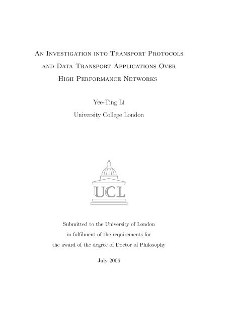
experiments. The Tiered hierarchy is shown in Figure 2.1, which also shows
the expected traffic volumes between Tiers.
• Tier-0

2.3. Data Volumes and Regional Centres 34
ATLAS
Experiment
Online
System
~PB/sec
~1.2-12 Gbps
Tier 0 (+1)
CERN
~10-40 Gbps
Tier 1
US
(Fermi)
UK
(RAL)
France
(IN2P3)
Italy
(INFN)
...
~10 Gbps
Tier 2
North
Grid
Scot
Grid
South
Grid
London
Grid
~1-10 Gbps
Tier 3/4
UCL Imperial RHUL ...
Figure 2.1: The MONARC hierarchy of Tiers for Atlas, with estimated initial data
transfer rates between the different tiers.
There is only one Tier-0 site. For LHC this is CERN, where the data
is acquired from the experiment, and initially stored. The first data
reconstruction occurs here, and CERN shares the work of the Tier-1
sites.
• Tier-1
Tier-1 Regional Centres will service a nation, or a group of nations.
They are expected to replicate as much of the data stored at CERN as
possible in order to facilitate access to the data with approximately 10
sites worldwide. Typically, the network provision between the Tier-0
site and Tier-1 sites should be high, deploying either multi-gigabit links
and or DiffServ and or MPLS solutions to guarantee flow protection.

2.3. Data Volumes and Regional Centres 35
• Tier-2
Tier 2 centres will service single nations or regions, caching popular
data in their local storage. There will be approximately 60 sites worldwide.
• Tier-3 / 4
The local computing resources at member institutions make up Tier-3
of the model, with Tier-4 consisting of individual machines.
The initial storage and processing of event data will be located at the Tier-
0 site. In the case of the LHC, this will be CERN. The data is then replicated
to various Tier-1 centers around the world where they are further processed.
Approximately sixty Tier-2 regional centers, each serving a medium-sized
country, or one region of a larger country (e.g. USA, UK, Italy, etc), will
then replicate data from the Tier-1 centers. Physicists will then typically
access and further analyse data using one of hundreds of Tier-3 and Tier-4
workgroup servers and/or desktops.
The design of such a system ensures that a physicist should not need to
wait more than 10 minutes [LN00] to transfer relevant data for analysis.
The estimated data rates between Tiers are based on having a very wellordered,
group orientated and scheduled approach to the transfer of data. As
such, the data transfer rates are expected to actually be higher in practice.
An important development in being able to realise the transport requirements
of such data intensive science applications is that of a shift from the
typical shared ‘best-effort’ services of the Internet to dedicated connection
oriented end-to-end paths to facilitate the separation (and hence impact) of
such large scale traffic to that of standard Internet traffic. This is apparent
in projects such as Terapaths [Gib04], OSCARS [Guo04] and LHCnet

2.4. Data Transfer Requirements 36
[BMMF05] where new technologies such as MPLS [RVC01, AMA + 99] and
DiffServ [BBC + 98] are being implemented across production local and wide
area networks.
This will allow the provision of network resource to form Hybrid Networks,
whereby end-users (typically large collaborations such as the LHC) will form
their own private (virtual) networks for the movement of large scale datasets.
However, this paradigm comes at at price as the overheads of installation,
configuration, support and maintenance must now be conducted by the
institutions rather than leased from providers. Therefore the utilisation of
such network resources are very important in order to provide a sufficient
return on investment.
2.4 Data Transfer Requirements
2.4.1 Tier-0 to Tier-1
The typical network connections between the Tier-0 and Tier-1 sites are
meant to be well provisioned to support efficient replication of data across to
different geographical Tier-1 sites. As Tier-1 sites will be located worldwide,
latencies will range from pan-European (around 20msec) to world wide distances
(around 200msec). As most of the infrastructure and investment will
be located between the Tier-0 and Tier-1 sites, there will be (at least initially)
a lot of spare capacity, and technologies such as MPLS/Diffserv may
be utilised to offer a greater Quality of Service (QoS) than ordinary traffic
[Gib04, Guo04] and also provide class protection to reduce the affect of such
traffic upon ordinary Internet traffic. Similarly dedicated light paths may be
leased for the sole purpose of continuous data transfer.

2.4. Data Transfer Requirements 37
2.4.2 Tier-1 to Tier-2
Traffic between Tier-1 and Tier-2 sites are likely to be relatively local, with
latencies in the range of 10msec to 50msec. Typical data transfers are likely
to pass through existing infrastructures such as that of Janet, Abilene etc
between the Tier-1 and Tier-2 sites. Currently most of these networks are
built upon 10Gb/sec backbones with relatively light loading (typically around
10% [ST]). If the network is shared (Internet), then it will be important to
maintain fairness between the LHC and commodity traffic.
2.4.3 Tier-2 to Tier-3/4
The ‘last hop’ of the LHC data transport will be from the Tier-2 centres to
that of local workgroup machines and desktop computers where physicists
will perform the analysis of data. As such, this will typically be what users
will perceive as the raw performance of the data transfer. Due to the locality
of the Tier-2 to Tier-3/4 sites, latencies are likely to be relatively small (less
than 20msec). However, the networks at this edge are generally likely to
be bottlenecked by the local MAN and campus networks, and will likely
need to be shared between all users on the campus and or local area and
thus fairness becomes an important issue. Therefore, is will be important to
sustain a balance between affecting other network users (and the network in
general) and achieving high throughput to enable the users to do their work.
2.4.4 Summary
Table 2.2 shows a matrix of TCP performance metrics according to the type
of end-to-end connection with a relation to that of the Tiers in the MONARC
architecture.

2.4. Data Transfer Requirements 38
Internet
Dedicated
(sole)
Dedicated
(shared)
Tier-0 to
Tier-1
1) Fairness
2) Throughput
3) Low Overhead
Tier-1 to
Tier-2
Tier-2 to
Tier-3/4
1) Fairness
2) Low Overhead
3) Throughput
1) Throughput
2) Low Overhead
1) Throughput
2) Fairness
3) Convergence
Time
Table 2.2: Overview of Transport requirements for different Tiers based upon the
type of end-to-end connection.
For an in-depth discussion of the definitions of the various metrics presented,
please refer to Chapter 7.
When the large scale data transfers are competing over the commodity
Internet, it will be very important that the transfer will not adversely affect
the existing traffic on the network, therefore the most important metric to
consider is that of Fairness. In order to aid efficient replication to the Tier-1
and Tier-2 locations, throughput becomes the next important factor to consider
such that very large scale caching will not be required at the Tier-0 and
Tier-1 sites respectively. It will also be important to minimise the amount
of data that needs to be retransmitted as such traffic on the commodity Internet
may lead to congestion collapse [FF99]. As such it is important for
the transport algorithms to have low overhead. This is especially important
at the bottom of the hierarchy due to the high possibility of bottlenecked
systems which are more likely to be located in Tier-3 and Tier-4 locations
(due to less hardware and or staff investment in tuning and optimisation).
When considering the move to dedicated circuits for the transport of LHC

2.5. Summary 39
data, the most important metric will be to obtain high throughput in order
to maximise return on investment. Associated with this will be the need to
maximise throughput by sustaining a low overhead as retransmissions will
reduce goodput. As there will be no competing traffic on dedicated circuits
the order of importance of the metrics is the same throughout all Tiers.
If the dedicated link were to be shared between a few network users (e.g.
parallel streams, or simultaneous replication of data to a few sites across the
same dedicated network 1 ), then the sharing of the throughput between the
flows is important. As such, fairness and to a lesser degree, the convergence
times become a factor.
2.5 Summary
An outline of the methods and data rates of particle physics experiments,
such as the LHC were given. The ATLAS experiment was presented and
the MONARC hierarchy was discussed. In particular, the conservatively estimated
data rates required for the replication and analysis of such data is
expected to be at least an order of a magnitude greater than current experiments.
As such, the idea of Hybrid networks was presented in order
to facilitate high transfer rates between Tiered sites, yet maintain segregation
between flows in order to prevent/reduce the impact upon commodity
Internet Traffic.
The relative importance of various evaluation metrics were also presented
within the LHC application and four unique areas were identified.
1 Due to the continued development of reliable multicast, the HEP community does not
currently consider it as a viable option.

Chapter 3
Background
Grid technologies [FKNT02, Fos01, FKT02] is considered as a major component
of enabling world-wide collaborative science, and of course, the Large
Hadron Collider (LHC) project.
Grid technologies are built upon existing technologies. They use Core
Middleware [FK97] that acts solely as a way of communicating to the underlying
Fabric [Fos01] to conduct Grid operations.
This Chapter looks into the medium on which Grid communication relies:
the Internet, and identifies that the TCP protocol imposes a bottleneck in
terms of high throughput data transfer.
3.1 Data Intercommunication
The need to transport data stored on computer systems around the world
is of fundamental importance in the application of the Grid. Without the
40

3.1. Data Intercommunication 41
movement of data to be processed, there would be very little point in having
a distributed Grid.
Fortunately, with the standardisation of the Internet [IET], much work
has already been done to enable seamless transfer of data from one system
to another. In this section, the paradigm of data transfer across the Internet
are discussed and the performance of the various layers that enable data
inter-communication are investigated.
TCP/IP
The TCP/IP protocol suite is commonly used by all modern operating systems.
TCP/IP [Ste94] is designed around a simple four-layer scheme. The
four network layers defined by the TCP/IP model are as follows.
Layer 1 - Link This layer defines the network hardware and device drivers
that refer to the physical and data link layers of OSI [Tan96].
Layer 2 - Network This layer is used for basic communication, addressing
and routing. TCP/IP uses IP and ICMP protocols at the network layer
and encompasses the network layer of OSI.
Layer 3 - Transport Handles communication among programs on a network.
TCP and UDP falls within this layer and hence is also equivalent
to the transport layer in OSI.
Layer 4 - Application End-user applications reside at this layer and represents
the remaining layers of OSI: the session, presentation and application
layers.
There are two main transport protocols that are commonly used today:
User Datagram Protocol (UDP) [Pos80] and Transmission Control Protocol

3.2. Network Monitoring 42
(TCP) [Pos81b]. The former offers a unreliable way of transferring information,
i.e. it does not know explicitly that a sent packet has been received,
whilst the latter offers a reliable service - for every packet of information
that is sent and consequently received by the receiving host, some kind of
acknowledgment is sent by the receiver and received by the sending host.
UDP can offer a greater raw performance as it does not require the extra
overhead of acknowledging information and maintaining state. However, as
UDP offers no kind of signaling from the network to discover the current network
conditions, it can be potentially dangerous if used maliciously (Denial
of Service attacks [MVS01, HHP03]).
As the Internet is based mainly on the connectionless communication
model of the IP protocol, in which UDP and TCP segments are encapsulated
before transfer across the internet, IP has no inherent mechanisms to
provide delivery guarantees according to traffic contracts and hence mechanisms
to reserve network resources have to be implemented via other means
(See Section 9.2). Because of this, IP routers on a given data path from
source to destination may suffer from congestion when the aggregated input
rate exceeds the output capacity.
3.2 Network Monitoring
3.2.1 Networking Metrics
Networking performances are broadly classified into both latency and throughput.
Moreover, other metrics such as the internet path (e.g. with traceroute)
[Jac89], the connectivity (whether the Internet host is reachable) [MP99] and
the jitter (AKA interpacket-delay variance) [DC02] may be important.

3.2. Network Monitoring 43
Whilst latency is an important metric, especially when applied to applications
such as voice or video conferencing, it is essentially constrained by
the physical (relative) location of the two hosts 1 .
As the majority of the
Internet is a shared resource with Best Effort [CF98] scheduling of resources,
consecutive pings may experience different latencies and hence cause jitter.
Similarly, the traversal of packets through different paths 2 may also increase
the jitter, so much so that packets may arrive ‘out-of-order’.
The transfer of bulk amounts of data involve the movement of many
packets of data. As such the microscopic effects of jitter and delay will also
affect the macroscopic effects of bulk data transport. Also, as the raw rate at
which data can be transfered is often a useful and readily measurable metric,
the issue of bandwidth monitoring has become an important indication of the
performance of many Internet applications. Unlike latency, which is limited
by physical constraints, such as the speed of light, the capacity (optimal
throughput) of hardware is limited by the clock frequency and protocols
used to control the medium - as defined by OSI Layer 2.
Two bandwidth metrics that are commonly associated with a path are
the capacity and the available throughput [LTC + 04]. The capacity is the maximum
throughput that the Internet path can provide to an application when
there is no competing traffic load (cross traffic). The available throughput,
on the other hand, is the maximum throughput that the path can provide to
an application, given the path’s current cross traffic load. Measuring the capacity
is crucial in calibrating and managing links. Measuring the available
bandwidth, on the other hand, is of great importance for predicting the end-
1 Delays caused by queuing at router and switches may also affect latency.
2 Both between routers and within routers themselves depending on router design/configuration.

3.2. Network Monitoring 44
to-end performance of applications, for dynamic path selection and traffic
engineering. A more user centric metric is the achievable throughput which
defines the actual throughput through the Internet of a real application.
For example, FTP [PR85] is a popular application level protocol designed
to transfer files across the Internet. Assume that the end-to-end path capacity
is 10Mbit/sec; because of competing users (because it’s a busy link)
the achievable throughput may only be 3Mbit/sec (as 7Mbit/sec is being
used by other users). However, upon initiating the FTP, the user may only
manage a transfer rate of 1Mbit/sec in steady state - which is the achievable
throughput due to the complex interaction of network buffers and user traffic
patterns.
3.2.2 Test Methodology
Assuming adequate hardware and driver configurations, back-to-back tests of
the transfer of data should be capable of high speeds. However, the TCP/IP
stack is composed of two different transport protocols that regulate the way
in which data is injected into the network. In order to determine the performance
limitations on inter-communication, the upper layers of the OSI and
TCP/IP stacks are investigated and these transport protocols are tested.
As mentioned previously, UDP is a stateless protocol that allows fine
control of packet data control. However, the transfer of data using UDP is
not recommended due to various reasons as outlined in Chapter 4. Therefore,
as most Internet applications work with the TCP transport protocol, it is
important to compare and contrast the performance of these two protocols.
Two hosts were identified to be the sender and the receiver of active network
traffic in order to determine the achievable throughput through a real

3.2. Network Monitoring 45
Internet environment. The hosts were equipped with Gigabit NIC cards and
the network path consisted of 15 hops as shown in Figure D.1 with a path
bottleneck capacity of 622Mbit/sec. The machines were chosen to give a representative
transfer rates achievable by real physics users wishing to transfer
data from CERN, in Switzerland, to Rutherford Appleton Laboratory, in
England, UK.
In order to generate UDP throughput traffic, UDPMon [HJ] was used and
configured to a inter-packet wait time of zero seconds (i.e. back-to-back
packets). For the TCP traffic, iperf [TQD + 03] was used to simulate the
transfer of data and appropriate provisions for a large socket buffer size was
used with a sufficiently large socket buffer size of 8MB at both ends (See
Section 5.1.1).
Tests were run over an entire week, with randomised start times. UDP
flows were conducted with 1,000 full sized packets and TCP was ran for 30
seconds. These values were found to be sufficiently long to reach steady state.
3.2.3 Results
Figure 3.1 shows the results of the tests and shows that whilst UDP was
able to achieve almost line rate with a mean throughput of 493Mbit/sec,
TCP was only able to achieve about half of that with a mean throughput of
195Mbit/sec. Therefore, there is a clear discrepancy in the performance at
the transport protocol layer.
Hardware performance bottlenecks between the two end-hosts can be assumed
to be negligible due to the successful transmission of UDP packets at
high speeds.
Similar tests to CERN from Manchester showed only marginal improve-

3.2. Network Monitoring 46
600
UDP
TCP
500
Throughput (Mbit/sec)
400
300
200
100
0
Tue
03 Sep
Wed
04 Sep
Thu
05 Sep
Fri
06 Sep
Date
Sat
07 Sep
Sun
08 Sep
Mon
09 Sep
Figure 3.1: Throughput across production networks using UDP and TCP Transport
Protocols between CERN and RAL in September 2002.
ments in the TCP throughput (approximately 30Mbit/sec more) with approximately
the same UDP throughput. This suggests that there is a performance
problem with TCP in being able to achieve the complete utilisation
of the path from CERN to the UK.
As such tests are intrusive and disruptive to network stability (See Section
4.1), UDPMon [HJ] was only configured to transfer 1000 packets in order
to calculate the UDP throughput. Whilst this is sufficient to determine the
transient state of the network, it may not provide a deterministic indication
of the state of the network for the 30 seconds that the TCP flows were
transferred for. As such, the longer duration of the TCP tests (compared to
the UDP tests), may be more prone to the effects of network cross traffic.
However, shorter TCP would not reach steady state due to the dynamics of
slow-start (See Section 4.3).
However, the transfer of UDP packets may provide an indication of the
router queue occupancy along the network path. As packets are typically

3.2. Network Monitoring 47
1
0.8
Bottleneck (fraction)
0.6
0.4
0.2
Network
Sender
Recveiver
0
0 50 100 150 200 250 300
Throughput (mbit/sec)
Figure 3.2: Bottleneck limits of TCP WAN transfers between CERN and RAL as
reported by Web100.
only lost when the network queues overflow, the consistent high throughput
of the UDP packets suggest that the average queue occupancy is low. Given
this information, it is expected that TCP should also be able to sustain high
throughput (on average).
To investigate the details of TCP transfers, all TCP results were passively
monitored using the Web100 [MHR03] framework in order to determine the
possible bottlenecks on the system. Web100 implements a facility whereby
the performance of TCP can be determined to be bottlenecked by either the
receiver, the sender or by the path in between. These variables are presented
in a ‘triage’ whereby the fraction between the three bottlenecks are logged.
Web100 is a Linux kernel patch that enables the in-depth logging of TCP
parameters. Figure 3.2 shows the result of the Web100 triage [MHR03] for
numerous network transfers (including those not presented in Figure 3.1) for
the network path shown in Figure D.1. The triage determines the bottleneck
associated with each transfer in terms of a ratio between the network, the
sender, and the receiver.

3.3. Summary 48
It clearly shows that that the network component is the overriding performance
bottleneck for TCP.
The structure of the graph show that there are certain operating regions
from the results at which the points ‘cluster’. This was found to be a result
of effect of socket buffers (See Section 5.1.1) which limit the physical memory
allocation to TCP, and hence the achievable throughputs.
3.3 Summary
Grid fabric components of storage and network hardware are investigated
and presented in Appendix A. In summary, the tests demonstrate that the
hardware potential for transferring data at greater than Gbit/sec rates is
perfectly feasible.
Test transfers across real production networks were conducted were conducted
using both the stateless UDP protocol and the standard TCP protocol
using memory-to-memory data copying between RAL in the UK and CERN
in Switzerland.
It was discovered that the UDP protocol consistently performed a lot
better than TCP, achieving on average about a factor of 2 difference in
throughput. As much of the Internet traffic relies on the reliable replication
of data across sites, TCP is a fundamental protocol in the performance
of all Internet-based applications. As such, further investigation as to why
TCP is incapable of achieving high throughput transport is warranted.

Chapter 4
Transmission Control Protocol
The movement of bits across a network requires both hardware and software
to co-ordinate the copying of data from one machine to another. The dynamics
and performance of this interaction is presented in the previous chapter
and in Appendix A. Real world transfers of data were conducted. It was
found that the performance of TCP from Switzerland to England was only
half that of the UDP protocol.
The Transmission Control Protocol (TCP) [Pos81b, Bra89, APS99] is the
most widely used transport protocol in the Internet and provides applications
with reliable, byte-oriented delivery of data on top of the stateless Internet
Protocol. In this chapter we look more closely at TCP to find out why it has
become the de-facto transport protocol on the Internet.
49

4.1. Overview 50
4.1 Overview
The Transmission Control Protocol was originally devised by Postel in 1981
[Pos81b]. Designed to enable inter-communication between disparate systems,
it is encapsulated above the stateless Internet Protocol [Pos81a].
IP routers connected on multiple network paths are shared resources
which may suffer from congestion when the aggregated input rate at any
networking node exceeds the output capacity. As there is no global signalling
mechanism to control the rate at which end-nodes send data into the
network, congestion can occur. Consequently, flows tend to experience varying
network conditions that affect the original traffic profile from the source.
This is known as Best-Effort servicing as each individual node tries its best
to forward packets without any service guarantees upon its performance.
Should all Internet users be using UDP as their primary transport protocol,
the aggregated input rate at any router would be greater than the
maximum output rate and overloading of Internet resources would take place
and potential Congestion Collapse [Nag84] would occur.
When congestion occurs, the amount of useful work done is diminished
to such a degree that the throughput declines and the network is termed
as undergoing congestion collapse. [FF99] and [MR91] outline the need for
mechanisms to prevent congestion collapse.
Congestion collapse is shown in Figure 4.1. It shows that as the sending
rate increases the useful work done increases linearly up to a point where
it reaches the network bandwidth. Past this point the throughput saturates
and the link pipes are filled and packets get queued at the routers. Similarly,
the delays experienced by the traffic increase due to the buildup of routers’
queues, and soon after the flows starts to lose packets. The loss can be re-

4.1. Overview 51
Throughput
Delay
Load
(a) Throughput
Load
(b) Delay
Figure 4.1: Congestion Collapse
covered by the sending hosts retransmitting them, but part of the bandwidth
will be wasted due to retransmissions.
At the turning point where the flow starts losing packets the amount of
useful work done by the network decreases dramatically and connectivity
diminishes completely; congestion collapse has occurred.
There are many types of congestion collapse [FF99]. Two of the most
common forms is congestion from the retransmission of packets already in
transit or that have been received (classical collapse), and that arising from
the transmission of packets that are subsequently dropped by the network
(congestion collapse from undelivered packets).
Originally devised to simply transport data reliably across networks [Pos81b],
TCP was adapted in 1988 by Van Jacobson [Jac88] to avoid network congestion
collapse and to provide network fairness between network users. Much
research, development and standardisation since its incarnation has led TCP
to be widely used in the Internet and it is considered as the de-facto standard
transport-layer protocol.
The achievements of TCP are most evident by the fact that the protocol
has changed little over the last two decades. With the advent of fibre optics

4.2. Protocol Description 52
TCP Segment
0 4 10 16
32 bits
Source Port
Sequence Number
Destination Port
Data
Offset
TOS
Checksum
Acknowledgement Number
Control Flags
Receiver Window
Urgent Pointer
TCP Options (variable)
Padding (variable)
Data (variable)
Figure 4.2: TCP header format.
and satellite communications, technological development has increased the
size of the Internet by orders of magnitude in terms of size, speed, load and
connectivity - and all this in the last couple of decades [CO01, CO99]. Even
with the wide range of network conditions present on the Internet, TCP has
been able to utilise and effectively share network resources between Internet
Users. More importantly, it is generally believed to have prevented severe
congestion collapse during this time [FF99, Nag84].
4.2 Protocol Description
The TCP header is shown in Figure 4.2. The source and destination ports
allow the hosts to identify multiple concurrent TCP flows at once. The
sequence and acknowledgment numbers facilitate reliable transport (See Section
4.2.2). The Receiver Window field is used for flow control (See Section
4.2.3). The Data Offset field provides a pointer to the start of the Data
field as TCP Options [Pos81b] are variable in size. The size of the Data field

4.2. Protocol Description 53
is dependent upon the Maximum Segment Size (MSS) of the TCP segment
and constrained by the MTU of the network path. The variable Padding field
at the end of the TCP Options is used to ensure that the TCP header ends at
a 32-bit boundary. Control Flags determine the type of TCP segment (e.g.
SYN, ACK, SYN-ACK, FIN, reset, or urgent) and denoted by either a true
or false bit for each type of segment (e.g. a SYN packet will have the SYN
bit marked, whilst a SYN-ACK will have both SYN and ACK fields marked).
The TOS field determines quality of service and enables packet level service
differentiation. The entire TCP segment is check-summed to facilitate the
detection of header and/or payload corruption.
4.2.1 Connection Initialisation
TCP connections are established between two hosts via a three-way handshake.
According to [Jac88], the sending and receiving of data after the
initialisation of the TCP connection is bounded by a packet conservation
principle; when this principle is obeyed, congestion collapse from excessive
data being put into the Internet will become the exception rather than the
rule.
The principle of packet conservation utilises the idea that data packets
cannot be placed into the network any faster than that at which acknowledgments
(ack’s) by the sender of the data are received. This is called ackclocking
and is an important property in maintaining a stable and even data
flow [VH97, Jac88, BPS99].
In the following we will give an overview of the features and implementations
that have made TCP such a success.

4.2. Protocol Description 54
Receiver's Advertised Window
Network Window
1 2 3 4 5 6 7 8 9 10
Data Sent
and ack'd
Data Sent
and waiting for ack
Waiting for window to
move before sending data
Figure 4.3: Sliding Window of TCP.
4.2.2 Reliable Data Replication
To ensure reliable in-order data replication between machines, a TCP sender
must maintain sufficient history of what data has been received by the TCP
receiver. The implementation of an acknowledgment system in TCP offers
such a mechanism by explicitly notifying the sender of what the receiver has
received.
This history is provided by implementing a window of bytes on the sender
which are currently ‘in-situ’ or packets in flight. Each byte of data is assigned
a unique sequence number and the sequence number corresponding to the
start of the data payload of each TCP packet is embedded in the TCP header.
The left-hand side of the window, snd_una, is advanced when the sender
receives an acknowledgment from the receiver. acks are cumulative in the
sense that the acknowledgment number in the header of each ack confirms
all bytes up to the given sequence number.
As data is not always delivered to the TCP receiver in a continuous way
(the network 1 can lose, duplicate or re-order packets) any data packets that
are not sequentially received at the receiver are called out-of-order data.
1 And potentially any layer directly underneath the transport layer.

4.2. Protocol Description 55
As a response to out-of-order segments, the TCP receiver sends duplicate
acknowledgments, dupacks, that carry the same acknowledgment number as
the previous ack it had sent - hence this does not change snd_una.
A sequential receipt of a number of dupacks signifies that a data segment
has potentially been lost in the network, and therefore the sender should
send the data segment (the left most side of the sliding window) again.
In combination with retransmission timeouts (RTO) (See Section 4.5.1)
that will resend segments should no acks that advance snd_una be received
within this RTO, acks provide reliable data delivery [Bra89] by informing
the sender of when data has (and implicitly, has not) been received by the
receiver. Similarly, when new data is sent into the network, the right most
pointer, snd_nxt, advances to the right. Therefore, the window ‘slides’ across
the range of sequence numbers as the transfer takes place. Through the evolution
of the data transfer, this window will slide across the entire byte range
of the relevant data to transfer and hence is known as a ‘sliding window’.
The macroscopic result of this is that for each and every TCP connection,
this window has to be maintained as part of the connection state in memory
in order to be able to keep track of the number of packets in-flight. The
Bandwidth Delay Product (BDP) defines the relation between the throughput
b, the round-trip latency T , and the size of the sliding window w required.
b = w T
(4.1)
The relation between w and the number of packets is defined by:
w = n × s (4.2)

4.2. Protocol Description 56
Where n is number of packets in flight, and s is the size of each packet as
limited by the MTU and MSS. As such, should the physical memory assigned
to the sliding window be restricted, then the number of packets in flight is
restricted and consequently the throughput is also restricted.
Another way of thinking about the BDP is that for a network capacity of
C (i.e. b = C), and an end-to-end latency of T , the required window in order
for a TCP flow to saturate the path is C × T . This is only valid when there
are no competing flows as the presence of network cross traffic is that the
available bandwidth of the network is less than C. However, the presence of
cross traffic may also increase the latency of the flow, and therefore there is
a balancing effect (of the decrease in bandwidth, but an increase in latency).
A full account of this is given in [JPD03].
4.2.3 Flow Control
To prevent a fast sender from overflowing a slow receiver, and hence causing
losses at the receiver (and wasting network resources), TCP implements flow
control [Tan96]. In order to prevent such an occurrence, in every ack the
receiver advertises to the sender its ‘receiver window’ (rwnd) which represents
the number of bytes available for buffering at the TCP receiver before it is
processed and sent up to the receiver Application.
Therefore, if the TCP receiver cannot process the incoming data at the
speed which is being sent, the value of rwnd sent will get smaller as the
socket buffer at the receiver fills.
Through the advertisement of rwnd, the TCP sender can prevent overflowing
the receiver by limiting its maximum allowed window size for transmission.
This mechanism provides a simple, yet elegant way of preventing

4.3. Congestion Control 57
excessive transmission of data which will be lost at the receiver.
4.3 Congestion Control
The implications of congestion collapse led to the first proposal for a transport
protocol which will help prevent congestion collapse [Jac88].
TCP utilises another window to determine the dynamic flow control required
of the heterogeneous networks and hence an estimation of the available
capacity in the network.
This congestion window (cwnd) is defined as the number of allowed segments
(or bytes) sent but not yet acknowledged (packets or bytes in transit).
As such, it is analogous to controlling the rate at which packets are allowed
into the network along the bottleneck of a given network path.
Whilst congestion control was not originally part of the original TCP
specification [Pos81b], it has become part of the standard TCP specification
since the introduction of TCP Tahoe (See Section 4.5.1).
The two specific algorithms that control the evolution of cwnd are defined
as follows:
4.3.1 Slow Start
The purpose of the slow start algorithm [Jac88] is to get the ack clock running
and to determine the available capacity in the network. It is a mechanism
to quickly find an operating point at which TCP can work. Therefore it is
invoked at the start of every TCP connection after the initial TCP handshake.
Starting with a conservative cwnd of one segments 2 , the TCP connection
2 Recent suggestions state that TCP may set its initial cwnd to two segments in light
of the increase in link speeds [AFP98].

4.3. Congestion Control 58
sends out as many segments as it can ensuring that the number of packets
in flight does not exceed cwnd. After approximately one RT T , the TCP
sender should receive an acknowledgment informing receipt of the data from
the receiver. For every non-duplicate ack received,
cwnd ← cwnd + 1 (4.3)
During slow start, this algorithm is equivalent to an exponential increase
in the cwnd size as it effectively doubles every RT T as one more packet is sent
out for every non-dupack received. This increase of cwnd is quite aggressive.
However, it enables the TCP connection to quickly reach a stable point for
congestion avoidance (See Section 4.3.2) to take place.
Slow start ends when a segment loss is detected or when the congestion
window reaches the slow start threshold, ssthresh (See Section 4.3.3).
4.3.2 Congestion Avoidance
Under the packet conversation principle, a TCP connection at equilibrium
will send new packets with the rate at which it receives acks. Under ideal
circumstances, this rate should reflect the rate packets are served by the
slowest link of the entire path, also known as the ‘bottleneck link’.
When a sender is operating at equilibrium, i.e. in steady state, it should
be able to adapt to changes in the condition of the path. More importantly, if
more connections (say from other users) start to use part of the path, any one
TCP flow should ‘back-off’ its transmission rate and be fair to other flows.
Similarly, should a connection terminate then the sender should attempt
to utilise the extra bandwidth. This is exactly what congestion avoidance
[Jac88] does, and is implemented through a simple algorithm such that it will

4.3. Congestion Control 59
probe for extra bandwidth by increasing its sending rate slowly, falling back
to a ‘safe’ sending rate should loss or excessive delay of an ack (an implicit
indication congestion) occur.
The implementation of such an algorithm is given below:
ACK : cwnd ← cwnd + 1
cwnd
(4.4)
LOSS : cwnd ← cwnd − 1 × cwnd (4.5)
2
Upon receipt of an acknowledgment, when in congestion avoidance, the
sender increases the cwnd by
1
cwnd .
Therefore, after about cwnd of acks,
the sender will be able to send one more packet due to this increase. This
mechanism allows TCP to ‘probe’ the network to determine if it has more
resources; if it does, then it will make use of the extra bandwidth by continuing
to increase cwnd; if not, after approximately RT T the sender should
either be able to determine packet loss from dupacks sent by the receiver or
through a RT O soft timer expiration (See Section 4.5.1).
Should a loss be detected, then the congestion avoidance algorithm of
TCP reduces cwnd by half 3 and hence reducing the number of packets inflight
from the connection. This will reduce the resources used by this TCP
connection and helps to prevent congestion collapse from occurring.
The value of cwnd is never allowed to be less than 1 packet.
It must be noted that the requirement to prevent congestion collapse is
that all end-to-end connections should have the same form of reactive congestion
control behaviour. Therefore, the requirement of preventing congestion
3 [APS99, Pos81b] actually specify that cwnd ← F lightSize/2, where F lightSize is
the amount of data sent, but yet unacknowledged. For simplicity, it is assumed that the
F lightSize is the same as the cwnd. This assumption is valid only when TCPs ack clock
is not broken.

4.3. Congestion Control 60
collapse is a distributed one whereby all transport protocol control algorithms
should react upon indication of congestion by decreasing their sending rates.
The algorithm that governs Congestion Avoidance is referred to as Additive
Increase Multiplicative Decrease, (AIMD) [CJ89], due to the form of
Equations 4.4 and 4.5.
4.3.3 Slow Start Threshold
The general characteristics of the TCP algorithm are an initial, relatively fast
scan of the network capacity using Slow Start, followed by a cyclic adaptive
behaviour of Congestion Avoidance that reacts to congestion by reducing its
sending rate, and then slowly increasing the sending rate in an attempt to
stay within the area of maximal transfer efficiency.
In order to determine the balance between the aggressive algorithm of
Slow Start and the steady-state congestion probing algorithm of Congestion
Avoidance, another variable, ssthresh is introduced and is used as follows:
if cwnd < ssthresh
do slow start
else
do congestion avoidance
This slow start threshold, ssthresh, is typically set to a large initial value
and updated upon loss detection. In other words, after loss, the value of
ssthresh is set to half of the number of packets in-flight.
Through continuing updates of the value of ssthresh, the TCP connection
is able to recover to a stable operating region of congestion avoidance
quickly using slow-start when a RT O occurs and then continue its conges-

4.4. Retransmission Timeout 61
tion avoidance regime from a ‘safe’ operating at half the rate at which loss
occurred.
4.4 Retransmission Timeout
As TCP requires the receipt of acknowledgments in order to slide the TCP
window and thus maintain the flow of data between the sender and receiver,
should ack’s not be received then the TCP sender will indefinitely stall.
In order to rectify this, TCP implements a Retransmission Timeout (RTO)
which is a soft timer which is re-initialised after the receipt of an ack. It is
assumed that an RT O expiry (i.e. a period where no acks are received) is
equivalent to packet lost and therefore the missing segment should be retransmitted
to facilitate reliable delivery and progress movement of the TCP
window.
The delivery of each segment of data may experience differing latencies;
it is therefore important to have a good RTT estimator in order to determine
an appropriate RTO.
[Jac88] presented a calculation of RT O by applying a filter such that it
takes into account the variation of the average RTT, in fact this exponentially
weighted estimator devised for Tahoe is still in use today. The RTO is
calculated using a smoothed estimate of the RTT, SRTT, and a variance
estimate, RTTVAR [PA00].
SRT T ← SRT T + 1 (RT T − SRT T ) (4.6)
8
RT T V AR ← V RT T + 1 (|RT T − SRT T | − RT T V AR) (4.7)
4
RT O ← SRT T + 4 × RT T V AR (4.8)

4.5. TCP Variants 62
This enables spurious packet delays to be absorbed into the time-out to
facilitate a good estimation of the RT O.
RTT measurements resulting from retransmitted segments are not included
[KP87] to avoid false positive RTO calculations.
Standard TCP implementations (such as TCP Tahoe - See Section 4.5.1)
only time-stamp a single packet per RTT to reduce the CPU load, and thus
only a single RTT measurement can be gathered per RTT which will limit
the robustness of the above algorithm. More accurate RTT samples can be
gathered by using using the TCP Timestamp option (See Section 5.2.1) to
facilitate a more robust RTO calculation.
4.5 TCP Variants
Whilst the basic design of TCP has changed little since its incarnation, various
adaptations to the basic flow recovery mechanism have enabled TCP to
adapt as the Internet has evolved.
The original specification in [Pos81b] implements only the sliding window
and flow control of TCP. Also a very basic RTO estimator was used.
This section describes the major implementations and alterations of the TCP
algorithm to the current state.
4.5.1 TCP Tahoe
Designed in 1988, TCP Tahoe by Van Jacobson [Jac88] extends the original
TCP by Postel [Pos81b] with five new mechanisms that have become de-facto
TCP mechanism: slow start, ack clocking, window dynamic adjustment,
fast retransmit and round-trip time variance estimation. All of these new

4.5. TCP Variants 63
mechanisms are still widely in use today in the all TCP implementations.
TCP Tahoe assumes that congestion signals are represented by lost segments
and that losses due to packet corruption are much less probable than
losses due to buffer overflows on the network.
As there is no explicit notification of packet loss through the ack mechanism,
TCP Tahoe introduces the notion whereby packet loss can occur if:
A TCP soft time-out occurs such that no acks have been received in a
period RT O since the last ‘normal’ ack was received. Therefore, the ack
clock has stopped. TCP Tahoe implements a more accurate calculation
of RT O.
Receipt of 3 dupacks The TCP connection is still active and there is still
ack clocking. A packet may have been lost but all successive packets
were delivered successfully.
The refinement of an accurate round-trip time estimator was also introduced
with TCP Tahoe (See Section 4.4).
The occurrence of an RT O timeout is taken as a signal of severe network
congestion and therefore the rate at which the TCP should send more segments
should be decreased to prevent network collapse. As such, the TCP
flow reinitiates the TCP connection in slow start so that the network conditions
can once again be probed to re-initialise the ack clock. By setting
cwnd to 1 packet, TCP Tahoe starts sending from a very low rate and only
if the network is capable of the extra traffic will the ack clocking reinitiate.
Fast Retransmits [Jac88] were proposed to reduce the long idle periods of
time during which the TCP on the sending host waits for a timeout to occur.
Fast Retransmit is a mechanism that sometimes triggers the retransmission

4.5. TCP Variants 64
20
15
cwnd
ssthresh
Detected Packet Loss
Timeout
cwnd (Packets)
10
5
0
0 5 10 15 20 25 30
Duration (RTT)
Figure 4.4: Time Evolution of Example TCP Tahoe Trace.
of a dropped packet sooner than the regular timeout mechanism and hence
improves packet loss detection. It does not replace regular timeouts; it just
enhances that facility and keeps the ack clock from failing.
Fast Retransmits are implemented via the detection of dupacks at the
sender.
It suggests that either a packet has been lost, or received out of
order 4 . Upon the occurrence of three consecutive dupacks, TCP Tahoe decreases
the sending rate and the inferred lost packet is resent.
The main
difference between TCP Tahoe and variants such as TCP Reno (see Section
4.5.2) is that upon loss detection through dupacks, cwnd is set to one
packet rather than half of the previous value.
As the mechanism to set
ssthresh still holds, the TCP connection always restarts in slow start (after
loss detection) until cwnd reaches ssthresh and then the linear additive increase
of the congestion avoidance mechanism occurs until the whole process
is repeated or the connection is closed.
Figure 4.4 shows a typical time based evolution of TCP Tahoe. The TCP
4 Later implementations such as TCP SACK can calculate the exact missing segment
based on extra information provided by the receiver to prevent the need to retransmit
already received data.

4.5. TCP Variants 65
connection initially starts off in slow start, until in the 4 th RTT packet loss is
detected and ssthresh is calculated as half of the number of packets in flight.
As TCP Tahoe always restarts the connection in slow start, cwnd is set to
1 packet and cwnd slow starts up to ssthresh. When cwnd ≥ ssthresh
the TCP connection enters congestion avoidance until packet loss is again
detected. The cycle continues until the 21 st RTT when a network timeout
occurs whereby ssthresh is recalculated and cwnd is set to 1 packet.
4.5.2 TCP Reno
In 1990, Van Jacobson refined the congestion control algorithm. He noted
that congestion control should do two things: prevent the pipe from going
empty after a loss (as if it doesn’t go empty, the TCP flow does not have to
spend time refilling it again) and correctly account for all data that is actually
in the pipe (as congestion avoidance should be estimating and adapting to
the rate).
As a consequence of this chain of thought, TCP Reno [Jac88] introduces
major improvements over Tahoe. It still maintains all of the features of TCP
Tahoe (such as the improved RT O calculation and slow start after a timeout)
but changes the way in which it reacts when a loss is detected upon duplicate
acknowledgments.
The concept is that should the network be heavily congested, the receipt
of acks will stop (as the receiver will not receive any data packets to respond
acknowledgments to). Therefore it is highly likely timeouts only occur when
the network undergoes heavy congestion, and that the receipt of dupack
signifies that the network is only moderately congested.
Therefore, the implementation of slow start after a Fast Retransmit in

4.5. TCP Variants 66
TCP Tahoe completely destroys the ack clock unnecessarily and is too conservative
in its rate reduction.
Given this assumption, under moderate loads the sender should be able
to keep on sending data since the flow still exists (as the equilibrium has not
been completely destroyed). However, the sender should be sending with less
vigour to utilise less resources in order to prevent congestion collapse.
As such, Reno introduces a mechanism called Fast Recovery [Ste97] which
should be activated after a Fast Retransmit.
Recall that Fast Retransmits
will cause the sender to retransmit the lost packet after receiving three
dupacks. However, under Reno, it will not fall back to slow start, but instead,
it should take advantage of the fact that the flow that currently exists
should keep on sending, but using less resources.
By using Fast Recovery, the sender calculates half the number of packets
in-flight just before loss detection. It sets ssthresh to this value and then
subsequently also sets cwnd to the same value, rather than to one packet as
in Tahoe 5 . As such, this forces TCP Reno to send fewer packets out and
therefore it has indeed reduced its utilisation of the network.
As ssthresh is also updated upon congestion, TCP Reno is therefore also
able to quickly revert back to congestion avoidance should a RT O expiration
occur (causing the TCP flow to enter slow start).
But the shrinking of cwnd means that the TCP flow has already sent out
all the packets that are contained within the window and therefore there is
no way of sending out new packets unless the window is forced to include the
new ones. As the receipt of dupacks under Tahoe does not move this window,
then the only way to shift the window is to (artificially) inflate the size of
5 Actually, it is set to half of the the number of packets in flight before the loss plus 3
packets to signify the data segments that have been acknowledged by the 3 dupacks.

4.5. TCP Variants 67
20
15
cwnd
ssthresh
Detected Packet Loss
Timeout
cwnd (Packets)
10
5
0
0 5 10 15 20 25 30
Duration (RTT)
Figure 4.5: Time Evolution of Example TCP Reno Trace.
cwnd upon each dupack received as each represents another data segment
which has left the network. Therefore, upon the receipt of each dupack, the
cwnd is inflated by one segment as each dupack signals the fact that another
packet has left the network.
When all the dupacks have been received (cwnd/2 packets corresponding
to the number of of packets that were in flight prior to the loss detection), the
next ack should be that caused by the retransmission and therefore should
acknowledge all packets. Upon the receipt of this normal ack, the sender
exits Fast Recovery and set its cwnd to ssthresh to maintain sending at a
rate which does not destroy the ack clock.
Therefore, under Reno, slow start is only invoked at the start of a TCP
connection and when a packet is timed out by the RT O, i.e. only when the
ack clock of the TCP flow has been destroyed.
Figure 4.5 shows a typical time evolution of TCP Reno. Slow start is
initiated whereby at the 4 th RTT packet loss is detected and ssthresh is
recalculated. Unlike TCP Tahoe, TCP Reno effectively sets cwnd to the value
of ssthresh after Fast Recovery. After this, congestion avoidance is initiated

4.5. TCP Variants 68
until packet loss is detected at the 9 th RTT, where Fast Retransmission and
Fast Recovery is again initiated. At the 19 th RTT, a timeout occurs and
again ssthresh is recalculated, but cwnd is set to 1 packet whereby slow
start is initiated until cwnd ≥ ssthresh.
4.5.3 Motivation for Improving Loss Detection
A fundamental problem is that TCP acks are cumulative; an ack confirms
reception of all data up to a given sequence number, but provides no information
whether any bytes beyond this number were received. Therefore
upon loss, the Fast Retransmit and Fast Recovery algorithms assume that
only the segment at snd_una is lost per window. This can result in the loss
of ack clocking and timeouts if more than one segment is lost.
Due to the prevalence of FIFO queues in the internet, losses often occur
in bursts [JS00]. As link speeds increase and the internet becomes more
geographically distributed, with more hops, TCP cwnd sizes are increased
to make use of available capacity. The result of this amalgamation is that
single packet loss within a window is rare and multiple losses within the same
window are more likely to be the observed effect.
When Tahoe and Reno experience multiple packet losses in a window of
data (usually in the order of half a window under heavily congested links),
Fast Retransmissions and Fast Recovery are invoked several times in succession
leading to multiplicative decreases of cwnd and ssthresh.
As this happens several times in succession, the left edge of the sending
window advances only after each successive Fast Retransmit and the amount
of data in-flight (sent but not yet acked) eventually becomes more than the
cwnd (halved by the latest invocation of Fast Retransmit). As there are

4.5. TCP Variants 69
no more acks to receive then the sender stalls and recovers from this deadlock
only through a timeout - which destroys the ack clocking and is only
recoverable through slow start. This has the impact of severely reducing the
throughput of the TCP flow.
Another problem of inducing multiple Fast Retransmits is that the source
retransmits packets that have already been correctly received by the receiver
which increases the potential for classical congestion collapse [FF99].
A more in-depth discussion with diagrams is presented in [FF96].
4.5.4 TCP NewReno
A modification of Reno led to TCP NewReno [FH99] which shows that Reno
can be improved without the addition of SACKs (See Section 4.5.5) but still
suffers without it. Here, the wait for a retransmit timer is eliminated when
multiple packets are lost from a window.
NewReno modifies the Fast Retransmit and Fast Recovery. These modifications
are intended to fix the Reno problems of multiple Fast Retransmits
and are wholly implemented in the sender side, in contrast to TCP SACK.
NewReno is the same as Reno but with more intelligence during fast
recovery. It utilises the idea of partial acks; when there are multiple packet
drops, the acks for the retransmitted packet will acknowledge some, but not
all the segments sent before the Fast Retransmit.
In TCP Reno, the first partial ack will bring the sender out of the Fast
Recovery phase and will require a timeout when there are multiple losses in
a window to recover from the losses, thus stalling the TCP connection. In
NewReno, a partial ack is taken as an indication of another lost packet and as
such the sender retransmits the first unacknowledged packet. Unlike Reno,

4.5. TCP Variants 70
partial acks do not take NewReno out of Fast Recovery and it retransmits
one packet per RTT until all the lost packets are retransmitted thus avoiding
the multiple fast retransmits from a single window of data [Flo94b].
The downside of this is that it may take many RTT’s to recover from
a loss episode, and enough new data must be present in order to keep the
ack clock running. Otherwise, re-initiation of the ack clock through a RT O
timeout is still necessary.
The modifications to Reno to enable NewReno are as follows:
Multiple Packet Loss
When first entering Fast Retransmit, the highest sequence number sent so far
is saved in the variable recover. Normal retransmission of data and the Fast
Recovery algorithm are run as normal. However, when a new ack arrives,
an additional check is performed to ensure that this ack covers the value of
recover. If the sequence number of the ack is less than that of recover,
then this ack is a partial ack and signals that another segment was lost from
the same window of data.
As such, TCP can retransmit the segment reported as expected by the
partial ack. There are two versions of NewReno algorithm which differ in
the way that the RT O is updated under this scenario [FHG04]. Under the
‘slow-and-steady’ variant, the RT O is reset on every partial ack. Whilst
with the ‘impatient’ variant the RT O is only set after the first partial ack.
Due to this RT O update, the impatient variant is more likely to be able
to recover quickly under very lossy conditions (or large cwnds) by resorting
to timeouts, whilst the ‘slow-but-steady’ variant will take approximately n
RTTs to recover (where n is the number of lost packets in the window)

4.5. TCP Variants 71
[Hoe96]. In both cases, the TCP connection only exits Fast Recovery if the
new ack’s sequence number is larger than recover.
False Retransmits
In order to prevent the retransmission of segments that have already been
received by the receiver 6 , the same recover variable as per the previous
discussion is used 7 . With the initial call into Fast Retransmit after a loss is
detected, the RT O is reset. Upon consecutive RT O’s, the highest sequence
number transmitted so far is also recorded into recover. By checking the
received acks against recover, the TCP sender is able to prevent having to
retransmit unnecessary data.
The sender comes out of Fast Recovery and Fast Retransmits only after
all outstanding packets (at the time of first loss) have been acked.
4.5.5 Selective Acknowledgments (SACKs)
With Selective Acknowledgment, SACK [MMFR96], the data receiver can
inform the sender about all segments that have arrived successfully, so the
sender need retransmit only the segments that have actually been lost. However,
TCP-SACK requires that both TCP senders and receivers be modified
to support SACKs.
In order to be backwards compatible with existing non-SACK TCP receivers,
SACK capability is negotiated during the TCP handshake. If neither
of the TCP hosts implement the TCP SACK option, then TCP-SACK behaves
the same as TCP Reno - with its associated problem with multiple
6 As retransmitted packets may also be dropped.
7 Note that the original ‘experimental’ draft of NewReno does not implement the check
against recover.

4.5. TCP Variants 72
drops within a window. To avoid this TCP NewReno was proposed (see
Section 4.5.4).
TCP-SACK has been shown to perform well even at a high level of packet
losses in the network [MM96].
SACK Blocks
SACK attaches detailed information called SACK Blocks in TCP Options
[Pos81b] on each and every ack. Each SACK block specifies a contiguous and
isolated block of data not covered by the TCP Cumulative Acknowledgment
field. Therefore cumulative SACK Blocks reports in the ack segments help
the sender to identify ‘holes’ in the sequence numbers at the receiver; on the
receipt of an ack containing the SACK Block, the sender can infer which
segments are lost and hence retransmit only those segments. Therefore,
SACKs enables a TCP sender to maintain an image of the receiver’s queue
and enables recovery from multiple losses per window within roughly one
RTT.
Each SACK block is described using absolute sequence numbers, with
two sequence numbers describing each block, each taking 4B:
1st Left edge of the block, i.e. the first byte of the block successfully received.
2nd Right edge of the block; i.e. the sequence number of the byte immediately
following the last byte in the block.
Given that the TCP options field is limited to 40B, the maximum number
of SACK blocks per ack is limited 8 to four. However, as it is expected that
SACK will often be used in conjunction with other TCP Options such as
8 Each TCP option has a necessary associated overhead.

4.5. TCP Variants 73
TCP Timestamps [JBB92] (See Section 5.2.1), typically only 3 SACK blocks
are expected in each ack.
The extra redundancy in having more than one SACK Block in each ack is
necessary due to the lossy nature of network paths and enables ‘robustness’
when acks are lost. It is therefore also important that the SACK option
always reports the block containing the most recently received segment, as
this provides the sender with the most up-to-date information about the state
of the network and the data receiver’s queue.
However, the unacknowledged segments can be treated in different ways
when accounting for outstanding data. The approach promoted by the IETF
is to consider all unacknowledged data to be outstanding in the network.
Holes within SACK blocks indicate potentially lost packets. However, they
may also indicate reordered packets. The method by which SACK is implemented
can be conservative or aggressive in the way it treats the holes
within the SACK blocks. The Forward Acknowledgments (FACK) algorithm
[MM96] takes the more aggressive approach and considers the unacknowledged
holes between the SACK blocks as lost packets and therefore retransmits
the data. The more conservative approach suggested by the IETF is
to consider all unacknowledged segments to be outstanding in the network.
Although the FACK approach can result in better TCP performance it may
increase the retransmission of unnecessary data.
How the sender uses the information provided by SACK is implementationdependent.
For example, Linux uses a Forward Acknowledgment (FACK) algorithm
[MM96] Another implementation is sometimes referred to as Reno+SACK
[MMFR96, MM96].

4.6. Summary 74
D-SACK
As an extension of the SACK mechanism, if a duplicate segment was received,
then the receiver should send an ack, containing as its first SACK block, a
reference to the duplicate data. Using SACK information and the D-SACK
extensions [FMMP00] it is possible to infer the amount of re-ordering on a
path and it is possible to make TCP more robust to re-ordering by using this
information to set the fast retransmit threshold depending on the reordering
detected on a path [BA02, ZKFP02].
4.6 Summary
The functions and implementation of the Transmission Control Protocol
(TCP) were presented and some of the key changes to its algorithms in order
to better utilise network resources upon congestion were given.
As the Internet is a shared resource of many end-nodes sending traffic
into a ‘black-box’ network, it is important that users do not send data into
the network such that congestion collapse occurs. Should the transport algorithms
not support a mechanism that is aware of the need for appropriate
use of these resources, then congestion collapse will invariably occur. An important
aspect of TCP is that it introduces the idea of ‘congestion control’ in
order to regulate the rate at which data is sent (and retransmitted) into the
Internet. Because of the success of the Slow Start, RT O calculation, Fast
Retransmit and Fast Recovery mechanisms, it is widely believed that TCP
in all of its variants has prevented the occurrence of Internet collapse.
TCP implements the notion of a congestion window, cwnd, which is the
protocols’ estimation of the rate at which the network can handle network

4.6. Summary 75
traffic for a particular connection. Depending on the network state determined
from the inference of packet loss through the heuristics of acks, TCP
adapts its cwnd. By increasing cwnd such that the rate at which new data
is put into the network is increased TCP is able to take advantage of extra
bandwidth available. And upon indications of network congestion, TCP is
able to quickly free up network resources.
However, in order to reach this ‘steady state’, TCP requires a mechanism
to quickly adapt to network conditions from which Additive Increase Multiplicative
Decrease (AIMD) can take place. This is implemented via a slow
start regime where the sending rate is doubled every RTT (as long as there
is no loss). In conjunction with a ssthresh variable, TCP is able to switch
between the aggressive slow start and congestion avoidance algorithms.
As TCP is a reliable protocol, TCP needs to deal with potential loss of
packets.
It also assumes that loss due to packet corruption is rare 9 TCP
infers the difference between the types of congestion by the arrival (or absence)
of acks from the receiver. Under heavy congestion, it is likely that no
data will get delivered, and therefore there will be no acks in response. To
detect packet loss because of this, TCP implements a RT O soft-timer that
will initiate the retransmission of the packet that it believes is lost. Under
moderate congestion, it is likely that only some segments will be lost, and
this is represented in the arrival of dupacks from the receiver.
Much of the developments of TCP in the past have been related to the way
in which it responds to packet loss detection. TCP Tahoe reacts the same to
both heavy and moderate congestion by reverting the TCP connection back
9 TCP performance suffers in environments where there exists high Bit Error Rates
(BER) (e.g. wireless/radio). However, the kind of BER considered in this dissertation for
the HEP community typically include high quality links optical interconnects which have
low raw BER of 10 −12 .

4.6. Summary 76
into slow start. However, this will result in the breaking of the ack clock
which is required for stable TCP connections and therefore would take a
few RTTs to get back into congestion avoidance. Therefore, TCP Reno was
devised to be able to differentiate moderate congestion and react by only
halving cwnd. This is called AIMD in reference to increase of cwnd by one
segment per RTT when probing and the halving of cwnd upon loss.
However, as connection bandwidths and end-to-end latencies of the Internet
increase, cwnd has to increase to retain enough state to enable the sliding
window mechanism required for reliable delivery of data. As this occurs, the
chance of multiple losses of segments in a single window increases.
Unfortunately, TCP Reno and TCP Tahoe do not handle such situations
well and each will successively call its corresponding loss detection mechanism.
The effect of this is the stalling of the TCP connection as it attempts
to retransmit what it thinks is lost in the network.
Two primary proposals were developed to facilitate the recovery of TCP
under multiple packet losses per window. Of the two, Selective Acknowledgments
(SACKs) allow the TCP sender to recover from the losses in the
order of just one RTT. However, it requires that both the sender and receiver
specially implement SACKs in order to operate. TCP NewReno, however,
only requires a sender side modification, but it will take an amount of time
related to the number of lost packets in order to recover. Otherwise, it will
require that a RT O timeout occur at the sender.
Overall, it can be seen that many changes have been made over time in
order to improve TCP’s behaviour with respect to congestion. In the next
Chapter, more recent modifications are considered with the aim of improving
performance in high-speed networks.

Chapter 5
TCP For High Performance
The role of TCP in network transport is an important one. Not only does it
provide reliable replication of data across a multitude of different networks,
but it also prevents congestion collapse.
This chapter looks into the current application of the TCP protocol, real
world implementation difficulties and the effect upon TCP performance.
5.1 TCP Hardware Requirements
TCP is often implemented in software. However, the design of the TCP
protocol requires certain constraints on physical hardware in order to operate
efficiently.
This section investigates the effect of physical hardware upon TCP performance.
77

5.1. TCP Hardware Requirements 78
5.1.1 Memory Requirements
The reliable data transport design of TCP requires that a sliding window’s
worth of data be stored in memory in order to maintain state about the TCP
connection. Without such knowledge, it would be impossible for TCP to be
able to replicate data reliably across a network. The amount of physical
memory allocated to this sliding window is called the socket buffer memory.
Should the assigned value of this socket buffer memory be less than the
required value of the sliding window for optimal TCP transfers, then the
performance of TCP suffers as it is starved of physical memory space to keep
history for the number of packets in flight.
This is true of both the sending and the receiving TCP end-points; the
TCP receiver must also have a large enough assigned socket buffer memory, or
else TCP’s flow control at the sender will restrict the throughput to maintain
a rate sustainable by the TCP receiver (See Section 4.2.2).
The amount of memory that needs to be allocated to the socket buffer
memory, on both the sending and receiving hosts, is related to the Bandwidth
Delay Product (See Section 4.2.2) [CJ89].
The effect on a TCP connection of having limited memory is shown in
Figure 5.1. The graph shows the statistically multiplexed result of running
various socket buffer sizes from the production network between CERN and
RAL using the machines and configuration as shown in Section 3.2.2. The
test consisted of 490 individual bulk transfers using iperf [TQD + 03] with
the socket buffer sizes configured as shown. The theoretical prediction of
the estimated throughput is shown. It can be seen clearly that with small
socket buffers, the throughput is proportionally restricted by the amount of
memory available to the TCP socket.

5.1. TCP Hardware Requirements 79
Goodput (mbit/sec)
1000
100
Socket Buffers From CERN (Switzerland) to RAL (England)
Mean
Median
Minimum
Maximum
Theory
10
10 100 1000 10000
Socket Buffer Size (KBytes)
Figure 5.1: Effect of limiting the socket buffer size on TCP goodput.
The typical socket buffer memory size for Linux and BSD systems is set
to 64KB. Depending on the latency and stable throughput of the TCP path,
one can see that TCP would perform abysmally over the example link and
that the throughput would be capped so that the TCP window fits within
the 64KB.
To address this problem, grid and network researchers continue to manually
optimise socket buffer sizes to keep the network pipe full, and thus
achieve increases of transport throughput by many orders of magnitude.
The amount of memory allocated to each TCP connection on Unix systems
can be changed using the standard Unix setsockopt() [Ste98] call.
However, under Linux systems, the kernel also imposes a limit on the maximum
size of the socket buffer memory that can be allocated for each connection.
As such system administrator privileges are often required to alter
this limit such that userspace applications such as FTP can utilise large(r)
socket buffer sizes.
This is achieved using the standard sysctl variables
net.core.rmem_max and net.core.wmem_max for the read and write socket
buffers respectively. Similarly, the default allocated socket buffer memory

5.1. TCP Hardware Requirements 80
for systems that do not implement the setsockopt() call can be given default
socket buffer settings as defined in the net.core.rmem_default and
net.core.wmem_default sysctl variables.
One may be tempted to assign large default and maximum values to the
socket memory to enable high speed TCP transfers over high BDP paths.
However, this could lead to performance degradation on servers as physical
memory may need to be swapped to and from disk if many such connections
are used. Servers can often have hundreds to thousands of simultaneous
network connections.
5.1.2 Network Framing and Maximum Segment Size
As the TCP/IP paradigm requires the transport of data packets across the
Internet, a fundamental question arises upon the size of each packet or segment.
However, there is an overhead cost due to framing and encapsulation
upon of each packet.
As the IP, TCP and underlying Layer 2 headers are often static in size, by
imposing a larger packet size it is possible to increase the raw data throughput
due to the relative decrease in header overheads. Large packets also result in
fewer interrupts at then end systems which can result in higher throughput
(See Section A.2.4).
However, with larger packet sizes, and with constant Bit Error Rate
(BER), the probability of packet corruption increases - although this issue
only becomes serious with wireless networks [BPSK96, Che01, CKPC03].
The Maximum Segment Size (MSS) [Pos83] is the size of the raw data
which TCP is allowed to store in each packet. To prevent problems due to
fragmentation at the IP level, the Maximum Transfer Unit (MTU) [MD90]

5.1. TCP Hardware Requirements 81
1000
800
12000
10000
1500B
9000B
Goodput (mbit/sec)
600
400
cwnd (packets)
8000
6000
4000
200
1500B
9000B
0
0 1000 2000 3000 4000 5000 6000 7000
Time (seconds)
2000
0
0 1000 2000 3000 4000 5000 6000 7000
Time (seconds)
(a) Goodput
(b) CWND
Figure 5.2: Effect of TCP performance with different MTU sizes.
is used to impose an upper limit on MSS.
These values do not prevent senders from placing larger packet sizes into
the network. However, large segments packets will be ‘fragmented’ [Cla82a,
ZRT95] into smaller packets to overcome the size difference. This imposes
the extra overhead of increased packet header sizes and a higher chance
of packets lost to BER. At the receiver, the individual fragments are then
reassembled to form the original packet. To over come the problems of packet
fragmentation, Path MTU Discovery is often conducted to determine the
appropriate segment sizes on the network [MD90, Lah00].
The effect of using large MTU’s is shown in Figure 5.2 based on tests run
on the DataTAG testbed (See Appendix C.3). TCP counts acknowledgments
by segments rather than by bytes. As such, in order to achieve the same
throughput, larger MSS flows only require a smaller value of cwnd as more
bytes are transferred per unit value of cwnd.
On the other hand, the transport of each large MSS segments requires an
increase in latency in order for routers and switches to transport the segment.
This could lead to a larger RT O which may have a negative influence on TCP
timeouts and hence lead to a deterioration in average throughput. However,

5.1. TCP Hardware Requirements 82
this effect should be negligible on long latency paths where the extra latency
of processing the larger segment is small compared to the end-to-end latency.
Further information can be found in [Ste94, MDK + 00].
5.1.3 CPU Requirements
A context switch requires that the CPU state needs to be stored and restored.
The transport of segments to and from a PC requires the context switching
of hardware and software control such that separate compute processes of
the operating system can gain access to the CPU resources.
Gigabit speeds require the transport of 1,000,000,000
8×1500
= 83, 333 packets per
second using standard MTU sized packets. This means that a packet needs
to be processed about every 12µsec.
As TCP uses feedback from acknowledgments, the TCP sender must also
process all incoming acks. This means that a TCP sender must send out data
and receive acks in order to enable reliable transport. Also, TCP requires
the extra processing overhead of the contents of acks in order to determine
what data needs to be retransmitted 1 .
At higher speeds, more packets need to be handled by the end systems
which results in higher CPU utilisation.
The overheads required in the context switching of interrupts can be
mitigated via interrupt coalescing (See Section A.2.4) and the use of advanced
queue management techniques such as NAPI (See Section 5.2.3). Using larger
sized packets (See Section 5.1.2) may also help reduce the CPU utilisation
as long as fragmentation does not occur.
Figure 5.3 shows the CPU load during individual TCP transfers between
1 Also SACKs prove to be a serious overhead in computational terms.

5.1. TCP Hardware Requirements 83
CPU Load (fraction)
0.9
0.8
0.7
0.6
0.5
0.4
0.3
0.2
0.1
CPU Requirements for Various TCP Throughputs
Sender Kernel
Receiver Kernel
Sender User
Receiver User
0
0 100 200 300 400 500 600 700 800 900 1000
Throuhgput (mbit/sec)
Figure 5.3: CPU utilisation with different TCP throughputs.
identical Dual Xeon 2.0Ghz PCs over the MB-NG private WAN (See Appendix
C.2). The configuration of both machines is presented in Table B.2.
The receiver is configured to simulate packet loss by dropping every n th
packet to achieve a desired throughput as determined by the response function
which limits the throughput of TCP based upon the loss rate experienced
(See Equation 5.7). As each TCP connection under Linux is handled under a
single processor thread, the benefits of SMP systems are limited, and this is
demonstrated by nearly 100% utilisation of a single processor at high speeds.
It was observed that the TCP receiver requires a higher CPU load than
that of the sender, with an almost linear relation. The sender, on the other
hand, requires more CPU at higher speeds (with a higher gradient at higher
throughputs), most likely to due to influx of ack packets that require extra
processing overheads (such as duplicate acks and SACKs).
Other research [tePM] confirms the approximate calculation that 1Ghz
CPU is required for each Gigabit/sec throughput when the performance is
restricted to end-node hardware rather than Internet performance.

5.2. TCP Tuning & Performance Improvements 84
5.2 TCP Tuning & Performance Improvements
5.2.1 Standardised Changes to TCP
Inadequate Window
The 16-bit TCP Sequence Number and Acknowledgment fields as proposed
in [Pos81b] imposes a maximum TCP window size of 2 16 = 64KB. Without
the Large Window extensions [JBB92], the maximum throughput of a TCP
connection is limited by the RTT as given by Equation 4.1. On a typical
long distance link with a RTT of 100ms, the maximum throughput of the
TCP connection is therefore limited to 64KB
100ms = 5.12Mbit/sec.
The TCP extension for large windows [JBB92] is implemented using a
3-byte TCP Option that defines an implicit scale factor to multiply the window
size as reported in each TCP packet. It increases the size of the TCP
advertised window to 32-bits and then uses a scale factor to carry this 32-bit
value in the 16-bit window field of the TCP header.
It is sent only in a
SYN segment at the TCP handshake and hence the scaling factor is fixed
in each direction when a new connection is opened. The maximum window
guaranteed is 2 30 -bytes which imposes a limit of 1GB.
The use of scaling the window imposes problems of sequence numbers
wrapping around and therefore the possibility of acking incorrect segments
in the window.
This is dealt with internally to ensure that the sequence
number is within 2 31 -bytes of the left edge of the window. Old acks are also
dealt with using PAWS and through the IP TTL field [Pos81a].

5.2. TCP Tuning & Performance Improvements 85
TCP Timestamps and PAWS
The Timestamp Option [JBB92] provides for timing of every packet inflight,
rather than only one per RTT as defined in the original specifications
[Pos81b]. This improves the RTT estimation and enables keeping a more
dynamic and accurate value for RTO and hence slightly quicker response to
TCP timeouts.
TCP Timestamps occupy 10-bytes and require the sender to place a current
timestamp into each packet sent out (including retransmissions) which
is then echoed by the TCP receiver in the ack.
The implementation of the Timestamps option is especially useful for
environments with very variable latencies such as wireless networks [LK02].
However, especially in wireless environments, the implementation has to be
balanced against the extra overhead of header information.
The implementation of a timestamp also enables extra protection against
potential wrap around due to the reuse of sequence numbers for long duration
transfers. [JBB92] defines the Protection Against Wraparound Sequence
Numbers (PAWS) algorithm that enables the checking to ensure that arriving
packets are valid in time for the connection.
The inclusion of the Timestamp option also enables low-level improvements
in processing TCP data packets at the receiver. This is referred to
as ‘Header Prediction’ [Jac90] and enables the receiver to quickly process a
TCP segment provided that the timestamp is larger than the previous one
recorded and that the sequence number is the next in sequence.

5.2. TCP Tuning & Performance Improvements 86
Initial Window Size
For short TCP connections that only transfer a small amount of data, the
rate of transfer is limited primarily by the amount of time spent in slow
start. TCP is currently defined to start a connection with an initial cwnd of
one. Therefore, by increasing this value to three segments rather than one,
the amount of data transferred at the start of the connection is improved
by a factor of three and the connection can therefore terminate earlier for
the same amount of data sent. However, due to the larger initial burst, a
connection across links with very small router buffers may experience loss
sooner and therefore resort back into congestion avoidance.
[AFP98] defines an experimental extension that allows an increase of the
initial window to three or four segments. However, the number of segments
sent after an RT O is still fixed at one segment.
However, for large file transfers that take a long time, the time saved by
having a larger initial window is irrelevant as TCP will most likely spend
most of its time in congestion avoidance.
5.2.2 Host Queues
The txqueuelen is a Linux sysctl variable that determines the maximum
number of packets that can be buffered on the egress queue of the kernel
before it enters the NIC’s device driver [ABL + 03].
Higher queues sizes means that more packets can be buffered and hence
not lost. This is especially important for TCP in the Linux kernel as the
overflow of this queue will cause immediate congestion control to be instantiated,
even though the packet is lost locally rather than on the network. The
Linux Web100 patch [MHR03] determines such action as SendStalls and

5.2. TCP Tuning & Performance Improvements 87
1
0.8
Graph of Sender RX Interrupt Effect on CPU
Sender Kernel
Receiver Kernel
Sender User
Receiver User
1
0.8
Graph of Receiver RX Interrupt Effect on CPU
Sender Kernel
Receiver Kernel
Sender User
Receiver User
CPU Load (fraction)
0.6
0.4
CPU Load (fraction)
0.6
0.4
0.2
0.2
0
0 20 40 60 80 100
RXInt (usec)
(a) Sender
0
0 20 40 60 80 100
RXInt (usec)
(b) Receiver
Figure 5.4: Effect of varying RX Interrupt values on CPU load.
can be deactivated using Web100’s net.ipv4.WAD_IFQ sysctl.
However, imposing a large txqueuelen may add to extra delays in the
transport of TCP segments due to extra queuing latencies that may be experienced.
This could result in large variations of RTT and hence result in
poor ack-clocking and spurious timeouts [LK02, GL03].
The default value of 100 for txqueuelen in the Linux 2.4 kernels has been
reported to be insufficient to maintain high throughput transport [ABL + 03].
Newer Linux 2.6 kernels implement a default of 1,000.
Similarly, at the receiving end of transport, packets will be queued, once
past the device driver, in a queue called max_backlog.
5.2.3 Driver Modifications
Interrupt Coalescing
By reducing the number of context switches required to process a packet,
CPU overheads can be reduced at the expense of increased latency upon the
incoming/outgoing packets.
Intel e1000 network interface card drivers enable interrupt coalescing in

5.2. TCP Tuning & Performance Improvements 88
granularity of 1.024µsec time slices. This value was varied to investigate
the effect upon CPU utilisation which was measured using the Unix time
command. Figure 5.4 shows the effects of varying the interrupt values on the
Intel e1000 (version 5.2.20) driver on back-to-back tests at 1Gb/sec using
TCP and iperf on the MB-NG testbed network (See Appendix C.2). In all
tests, it can be seen that the most intensive component of CPU utilisation
is that of the kernel process, which involves both the memory handling and
packet interrupts.
Figure 5.4(a) shows the effect of changing the coalescing values on the
sender only, with the receiver set to interrupt on every packet (RXIntValue=0).
It clearly shows the reduction of CPU load on the sending machine as it approaches
23µsec - which is equivalent to approximately 2 packets (in this
case acks) that are received back-to-back due to the use of ABC (See Section
5.2.4) which causes two data packets to be sent back-to-back. As the
receiver is constantly interrupting on every (data) packet, its CPU utilisation
remains constant.
Figure 5.4(b) shows the effects of adjusting the receiver’s RXIntValue. It
can be seen that a small change of this value to approximately the time taken
to process one packet can reduce the CPU utilisation of the kernel by about
half. As it is now the sender which is interrupting on each packet, it can be
seen that there is also the benefit of lower CPU utilisation on the sender at
the same settings.
Figure 5.5 shows similar tests but varying the transmitting TXIntValue
coalesce value rather than the receiving.
It was observed that altering the TXIntValue on the receiver has no effect
on the CPU utilisation of either system. This is due to the fact that even
though ack clocking is important to TCP, it does not affect the number

5.2. TCP Tuning & Performance Improvements 89
1
0.8
Graph of Sender TX Interrupt Effect on CPU
Sender Kernel
Receiver Kernel
Sender User
Receiver User
1
0.8
Graph of Receiver TX Interrupt Effect on CPU
Sender Kernel
Receiver Kernel
Sender User
Receiver User
CPU Load (fraction)
0.6
0.4
CPU Load (fraction)
0.6
0.4
0.2
0.2
0
0 20 40 60 80 100
RXInt (usec)
(a) Sender
0
0 20 40 60 80 100
RXInt (usec)
(b) Recevier
Figure 5.5: Effect of varying TX Interrupt values on CPU load.
of data packets that are injected into the network if the acks are slightly
delayed. The effect of varying the transmit interrupt on the sender is that
there is an initially high CPU requirement as the the driver attempts to
interrupt for every packet (

5.2. TCP Tuning & Performance Improvements 90
5.2.4 Delayed Acknowledgments & Appropriate Byte
Sizing
At high throughput rates, TCP receivers would send a lot of acknowledgement
packets on the reverse path of the bulk transfer to facilitate ack-clocking
and to slide the TCP window. Under bulk one-way transport, acks are often
composed of an empty TCP packet (with only header information), and
are therefore normally quite small (56B). As demonstrated in Section A.2.3,
small packets can pose a serious processing burden on both the end-host and
the intermediate switches and routers.
As acks cover all segments prior to the sequence number within the ack,
the advancement of the TCP window is not diminished by reducing the
number of acks sent by the TCP receiver [Cla82b].
Under delayed acknowledgments [Cla82b, APS99], a TCP receiver does
not acknowledge a received segment immediately, but waits for a certain time
(typically 500msec). If a data segment is sent from the receiver during this
time (i.e. as with two way communication), the acknowledgment is piggy
backed into it. Alternatively, if another data segment arrives from the TCP
sender, then the receiver will send a single ack that confirms both segments
at once.
It is suggested by the IETF that delayed acks should be incorporated
into TCP implementations [Cla82b]. However, the consequence may be that
‘stretched’ acks result that will acknowledge more than two full-sized segments.
This would lead to potentially large line-rate bursts of traffic [Pax97]
(which can also occur with large amounts of ack loss).
Typically each arriving ack at the sender advances the sliding window
and increases the congestion window by one segment; thus, a connection with

5.2. TCP Tuning & Performance Improvements 91
500
50
450
45
400
40
Cwnd (packets)
350
300
250
200
150
Goodput (mbit/sec)
35
30
25
20
15
100
Normal Acking
50
Delayed Acking
Delayed Acking with ABC
0
0 50 100 150 200 250 300
Time (seconds)
10
Normal Acking
5
Delayed Acking
Delayed Acking with ABC
0
0 50 100 150 200 250 300
Time (seconds)
(a) CWND
(b) Goodput
Figure 5.6: Effect of delayed acks upon cwnd dynamics.
delayed acks is less aggressive, and increases cwnd at half the rate compared
to a TCP connection without delayed acknowledgments.
This results in
reduced throughput over short timescales after each congestion event for any
TCP connection where the receiver is using delayed acknowledgments. This
is shown in Figure 5.6 for machines on a private dummynet network (See
Appendix A.5).
This is especially noticeable in the slow start phase, because in slow start
each arriving ack increases the congestion window by one segment, thus
effectively doubling the rate at which packets are sent.
The Linux kernel implements delayed acking by default [Bra89], but imposes
a less conservative delayed acking time of up-to 200ms. Linux introduces
a feature called quick acks [SK02] which helps to reduce the problems
of reduced responsiveness when using delayed acking during slow start. The
idea is to disable delayed acks at the receiver for the first n packets of the
connection, where n is a configurable parameter, acknowledging every packet
at the beginning of the connection and thus achieving the equilibrium state
(congestion avoidance) in shorter time.
On the other hand, such a policy would increase the probability of net-

5.2. TCP Tuning & Performance Improvements 92
work congestion on the reverse path as more acks are put into the network.
However, as quick acks are designed primarily to reduce the time required for
slow start to complete, the number of quick acks is calculated as n =
rwnd
2×MSS
where rwnd is the reciever advertised window and MSS is the maximum segment
size of the connection. This value, n, corresponds to the number of
packets that the TCP connection should take to exit slow start.
Appropriate Byte Counting (ABC) is a technique to eliminate the slow
growth of cwnd with delayed ack receivers and is outlined in [All03]. It gives
details of how TCP senders should behave when updating their congestion
windows through byte counting rather than the more common packet counting.
This has the benefit of improving TCP responsiveness without increasing
the amount of ack traffic (relative to the throughput) upon the reverse path.
Figure 5.6 shows the effect of running an ABC enabled sender when transferring
data to a normal delayed ack receiver. It can be seen that the dynamics
of using ABC is similar to that of a TCP sender sending data to a
receiver with delayed acks disabled.
It can also be observed that the queueing is apparent as the goodput
remains constant as the cwnd continues increasing until finally the buffer
overflows and fast retransmit and fast recovery takes place.
A potential consequence of implementing ABC is an increase in the burstiness
of the TCP traffic as two back-to-back data packets are sent for every
delayed ack [All99]. In order to reduce the effects of multiple packet bursts,
especially during slow start, a limit L, is introduced that limits the number
of full sized segments that the cwnd will advance by for each delayed or
stretched ack [All03]. The value of L= 2 means that a maximum of 2 new
segments are sent for every one delayed ack received.

5.2. TCP Tuning & Performance Improvements 93
5.2.5 Dynamic Right Sizing & Receiver Window
When the TCP sender’s window is not constrained by the system socket
buffer size nor by the congestion window, it will be throttled only by the receiver’s
advertised window (as per TCP flow control). The size of the receiver
window is a standard control parameter of TCP [Pos81b]. By advertising a
smaller window the receiver can control the number of segments that the
sender is allowed to transmit (similar to imposing a small socket buffer at
the sender).
[FF01] describe modifications to the Linux kernel that allow the kernel to
tune the buffer size advertised by the TCP receiver. Called Dynamic Right
Sizing (DRS), the receiver’s TCP kernel estimates the bandwidth from the
amount of data received in each round-trip time and uses that estimation to
derive the receiver’s window to advertise back to the sender. Assuming that
the sender is limited only by the network condition (i.e. by its cwnd value),
then the amount of data transferred in approximately one RTT is equal to
one windows worth of data. Therefore, by the TCP receiver measuring the
time taken to receive one windows worth of data, it can determine the RTT of
the connection. This value of RTT is used as an upper bound on the latency
of the link and therefore the appropriate receive window size to advertise in
following TCP acks.
Therefore, the effect of DRS on TCP senders is that their cwnd value
is never allowed to grow beyond what is actually achievable through that
connection and is clamped to the value as calculated by the TCP receiver. As
such, the TCP flow never actually imposes the additive increase of congestion
control and hence does not impose the necessary loss that is typical of the
oscillatory behaviour of TCP.

5.2. TCP Tuning & Performance Improvements 94
1400
cwnd
ssthresh
1400
cwnd
ssthresh
cwnd and ssthresh (packets)
1200
1000
800
600
400
cwnd and ssthresh (packets)
1200
1000
800
600
400
200
200
0
0 5 10 15 20 25 30
Time (seconds)
(a) Normal
0
0 5 10 15 20 25 30
Time (seconds)
(b) DRS
Figure 5.7: Effect on cwnd with Dynamic Right Sizing.
This behaviour is especially important for long-distance, high throughput
environments where the Multiplicative Decrease of TCP upon congestion/loss
causes a halving in throughput. Another benefit of using DRS is
that with appropriate socket buffer sizing (see Section 5.1.1) it also keeps the
amount of memory utilised to the minimum required for each flow.
Figure 5.7 shows the behaviour of the sender cwnd with and without
DRS along the MB-NG testbed (See Appendix C.2) with periodic loss on the
forward path. MB-NG has a RTT of 6.2ms with 1Gb/sec connectivity. As
such, the Bandwidth Delay Product (BDP - Equation 4.1) is approximately
535 packets.
Figure 5.7(a) shows the effect of queueing resulting in the curved cwnd
graph as the router queues begin to fill 2 . The initial plateau of cwnd in
Figure 5.7(a) is caused by socket buffer limitations at the sender which enable
flow control by capping the maximum value of cwnd. Figure 5.7(b) shows the
same network and dropping probability, but this time with DRS enabled at
the receiver. It can be clearly seen that the cwnd value is capped to that of
2 Note that in this case, the actual loss is imposed by the receiver selectively dropping
packets rather than the network.

5.2. TCP Tuning & Performance Improvements 95
the BDP of the network at just under 600 packets, which is the maximal rate
at which the receiver is able to receive packets as the sender is transferring
data at line rate.
It is clearly visible that the oscillatory behaviour of TCP is minimised
such that the sustained throughput is higher. However, it should also be
noted that due to the drop in cwnd upon loss, the utilisation of a DRS’d flow
is not maximal as with the case of normal TCP. The advantage of imposing
such an algorithm is two-fold: with appropriate measures to minimise the
socket-buffer size to that actually used by the flow (i.e. approximately the
value of cwnd) memory is not wasted; and induced loss through sending too
many packets into the network is also minimised, and therefore should the
buffer provision be small along the path, a DRS’d flow should be able to
obtain higher utilisation than a normal flow.
5.2.6 Socket Buffer Auto-Tuning & Caching
[SMM98] describes modifications to a NetBSD kernel that allow the kernel
to automatically resize the sender’s buffers. It enables a host that serves
many clients (such as a web server) to fairly share the available kernel buffer
memory and to provide better throughput than manually configured TCP
socket buffers. This is called socket buffer autotuning and is important as the
assignment of large default socket buffer sizes for all TCP connections would
result in the reduction of physical memory.
For applications that do not explicitly set the TCP send buffer size via
the setsockopt() options, socket buffer autotuning allows the sender socket
buffer to grow with cwnd and utilise the available bandwidth of the link
(up to the receiver’s advertised window). As the number of flows increases,

5.3. Network Aid in Congestion Detection 96
consuming physical memory, the kernel also facilitates the reduction of the
sender’s socket buffer window sizes to reduce the burden of memory swapping.
The modification of socket buffer auto-tuning algorithm were ported to
the Linux 2.4 kernel in 2001 and are controlled by new kernel variables
net.ipv4.tcp_rmem and net.ipv4.tcp_wmem defining the minimum, default
and maximum socket buffer memory allocated to each TCP connection for
the read and write buffers respectively 3 .
Independent of auto-tuning, the Linux 2.4 and 2.6 kernels implement a
system where connection performance histories of TCP transfers are cached
for up-to 10 minutes. This ‘retentive’ TCP stores details of the measured
/ experienced smoothed RTT and RTT variance, ssthresh and the path
reordering information for previously connected pairs of hosts. These values
are stored for up-to 10 minutes and will prevent a consecutive TCP flow for
that pair to reach congestion avoidance quickly without the excessive packet
losses of a typical slow start. It will also aid in preventing early spurious
timeouts. The cache can be prematurely cleared through the use of the
net.ipv4.route.flush sysctl.
5.3 Network Aid in Congestion Detection
Due to the transient nature of network utilisation, TCP gently probes the
network with increasing number of segments to determine whether it can
achieve more throughput. Therefore, in a sense, TCP has to cause congestion
in order to determine the capabilities of the network path.
Most current routers in TCP/IP networks do not detect incipient conges-
3 Note, however, that the maximal tunable socket buffer memory is still limited
by the maximum allocated socket buffer size in the kernel under net.ipv4.tcp mem,
net.core.rmem max and net.core.wmem max.

5.3. Network Aid in Congestion Detection 97
tion. When a queue overflows packets are dropped, and reliable transport
protocols, such as TCP, will attempt to retransmit missing data.
The design of router queue provisioning is often not to increase the utilisation
of a single flow going through their network, but that of the aggregate.
Given this and the limited resources of physical memory, it is often
not possible to provision large buffers required for high throughput, high
latency transport as required by Equation 4.1 and Equation 5.4.1. Also,
with the increased popularity of VoIP and similarly delay sensitive flows
[KBS + 98, JS00], it may not be feasible to utilise a large buffer, which is necessary
for efficient high throughput transport due to the increased end-to-end
latencies of large router queues. More important, however, is that a small
queue is insufficient to handle the bursts of packets that are commonplace
on the Internet [LTWW94].
This section looks at providing feedback and queueing disciplines from
routers that may improve the performance of TCP.
5.3.1 Explicit Congestion Notification
In TCP, a packet loss is an implicit notification of congestion. Through the
signaling of an Explicit Congestion Notification (ECN) [RFB01] packet, the
TCP sender should reduce the sending rate to mitigate the possibility of
congestion.
Designed to be complemented with Active Queue Management techniques
(see Section 5.3.2) on routers, ECN is implemented as the last two bits of
the IPv4 TOS octet in the TCP header and implemented such that TCP can
respond to congestion without actually suffering from packet losses.
When experiencing the incipient stages of congestion, an ECN enabled

5.3. Network Aid in Congestion Detection 98
router should mark the TCP packets with a Congestion Experienced (CE)
bit pattern and then process it normally. Upon receipt of a packet containing
the ECN codepoints, the TCP receiver should echo back the same bit pattern
in its acks. Should the received packet contain a CE-bit marked, the TCP
receiver should also set an internal flag to indicate that all subsequent acks
should also have the CE-bit set to 1.
When the TCP sender receives a CE marked ack, it should immediately
reduce the transmission rate according to congestion control principles. However,
the signaling of many CE packets must be handled such that TCP reacts
at most once per window (or approximately once every RTT) to prevent
successive reductions in cwnd [Flo94a].
The TCP sender, after reducing its transmission rate as a consequence
of a CE packet, marks the Congestion Window Reduced (CWR) flag in all
subsequent data packets on the first bit of the ECN codepoint. The TCP
receiver will only stop sending CE marked acks once it has received a packet
with the flag CWR.
The use of this field requires that all routers, switches and firewalls must
not modify packets with ECN-bits unless the node is under congestion. Also,
nodes that do not implement ECN should still pass ECN bits unaltered and
should not consider packets with ECN bits set as malformed and drop the
packets.
ECN has the obvious advantages in avoiding unnecessary packet drops
due to lack of memory. It also avoids the excessive delays necessary for
duplicate acknowledgments and retransmission timeouts. Indeed, experimental
validations of ECN have shown that TCP achieves moderately better
throughput [H.K98, SA00]. It also enables the efficient usage of bandwidth on
the forward path of the data transfer and hence improves the responsiveness

5.3. Network Aid in Congestion Detection 99
of the TCP flow when a high fraction of losses is less likely.
5.3.2 Active Queue Management & Random Early Detection
The prevalence of drop-tail routers in the Internet can result in ‘lock-up’
[FJ92] and the unfair sharing of network resources. The former occurs when
a high throughput flow starves other competing (possibly lower throughput)
flows of any queue occupancy due to the fact that a higher throughput flow
is more likely to have a larger number of packets in an ingress queue. When
‘lock-up’ does not occur, higher throughput flows still occupy a majority of
the queue, hence being unfair to other flows sharing the bottleneck.
The Random Early Detection (RED) [FJ93] algorithm solves the problems
of over-buffering and fair sharing of buffer resources. [BCC98] recommends
that RED is used as the default queue management algorithm on
the Internet as there apparently no disadvantages and numerous advantages
[FJ93].
Active queue management attempts to prevent queue overflow by selectively
dropping packets in a queue. It also has the advantage that TCP flows
do not have to induce a buffer to overflow as an indication of the congestion.
RED is termed an Active Queue Management solution as a RED enabled
router detects the incipient stages of congestion by observing the exponentially
weighted moving average of the queue size.
Defined with minth and maxth, the two values define the thresholds from
which no packets should be dropped and where all packets should be dropped
respectively. Therefore, the average queue occupancy, q, should fall within
minth and maxth. This enables the unavoidable bursts of packets in the Inter-

5.3. Network Aid in Congestion Detection 100
1
Drop Probability
max p
0
min th
max th
Average Queue Length
Figure 5.8: Random Early Detection Parameters.
net [BCC98] to be accommodated without any bias. The above parameters
are combined with maxp which sets the maximum probability that a packet is
to be dropped at the router. It is defined as a function of the average queue
size and is set to a linear dropping probability from 0 to maxp,whereby arriving
packets are marked depending on q. Should q be less than minth
upon an arriving packet, the packet will be processed normally. However,
if q is greater than maxth, then the packet will be dropped. Otherwise, the
incoming packet will be dropped according to the probability related to the
average queue occupancy. This is shown in Figure 5.8.
Therefore, the router selectively drops packets from the queue based on
the various parameters and occupancy of the queue. RED is able to achieve
fairness between flows as higher throughput connections will have a greater
occupancy in the queue, and hence a greater chance of packet drops.
The use of RED can also reduce the possibility of TCP synchronisation
whereby all flows experience drops at the same time and then simultaneously
increases their rates, only to cyclically have all flows experience packet loss.
The occurrence of synchronisation results in poor throughput and low link
utilisation [ASA00].

5.4. Analysis of AIMD Congestion Control 101
RED is wholly implemented on routers and therefore requires no modification
on TCP hosts. The exception is when RED is used in conjunction with
ECN (see Section 5.3.1) whereby a marked packet will be set to include the
CE-bit rather than be physically dropped by the router in order to mitigate
congestion.
5.4 Analysis of AIMD Congestion Control
For bulk transport of data, the dominant factor in the rate at which data is
transported is the congestion avoidance algorithms of TCP. Unfortunately,
the congestion control mechanisms of TCP constrain the congestion windows
that can be achieved by TCP in realistic environments, and hence the
achievable throughput.
The performance of a very long bulk transfer TCP connection is dependent
on the packet loss rate, bandwidth and round trip time, and of a connection.
These are considered in turn:
Packet Loss Rates Standard TCP implementations can only reach the
large congestion windows necessary to fill a an end-to-end path with a
high bandwidth delay product when there is an exceedingly low packet
loss rate. As standard TCP implementations cannot distinguish between
real network loss (e.g. corruption) and losses due to network
congestion 4 , the underlying physical network has to be able to maintain
very low loss rates in order for TCP not to invoke congestion avoidance
when a packet is lost through corruption rather than congestion.
4 Without network feedback such as ECN which would require deployment throughout
bottleneck routers.

5.4. Analysis of AIMD Congestion Control 102
For example, in real life systems, a packet loss rate of about 10 −7 is
comparable to the random losses that occur in long haul fibres, routers,
switches and end-systems. This physical limit imposes an absolute limit
on the throughput that a TCP connection can achieve - even without
competing traffic on the end-to-end path (see Section 5.4.2).
Bandwidth The higher throughput that the TCP connection has to sustain,
the larger its cwnd for the connection. With the implementation of the
current Additive Increase of 1 segment per round-trip time, TCP probes
for extra network capacity slowly, and therefore is unable to effectively
use available network resources that are present on high bandwidth
networks that are not fully utilised.
Also, the detection of packet loss through congestion or network corruption
in TCP results in a halving of its cwnd. When high speeds are
reached this mechanism of Multiplicative Decrease by half leads to a
significant decrease in the throughput of the TCP connection.
As TCP congestion control is cyclic (i.e. it will continue to slowly
increase its sending rate until congestion/loss is detected, where upon
it will halve the rate) the overall utilisation of the link by a single TCP
flow could be low compared to the capacity of the bottleneck link on
the path.
Round-Trip Time TCP utilises acknowledgments to update its window
based algorithms. This provides a feedback loop that drives the linear
increase of cwnd to increase its throughput. As the round-trip latency
increases, the time required for this feedback also increases. This results
in a slower rate of increase (in absolute time) of cwnd and therefore a

5.4. Analysis of AIMD Congestion Control 103
slower rate of throughput increase.
This is especially evident after congestion as TCP halves cwnd. Therefore,
when a TCP connection runs over a low loss, un-congested link it
is unable to achieve high throughput in high-speed, wide area networks
due to the long recovery times and large value of optimal cwnd required
after congestion detection when cwnd is halved.
Therefore, as the geographical distance of the TCP connection increases,
the time required to reach congestion (assuming static networks
conditions) is proportionally increased and its average utilisation
is decreased.
To give context to these problems, a standard TCP connection with 1500B
packets and a 100ms round-trip time (typical trans-Atlantic connection),
would require an average congestion window of 83,333 segments and a packet
drop rate of at most one congestion event every 5 billion packets to achieve a
steady-state throughput of 10Gbit/sec. This requires at most one congestion
event every 1 hour and 40 minutes. This loss rate (which is assumed to be
related directly to the Bit Error Rate) is well below what is possible today
with the present optical fibre and router technology.
5.4.1 Throughput Evolution
A model of the algorithmic dynamics of TCP can be gathered through simple
geometry when considering the steady state behaviour of TCP as a cyclic
iteration over k congestion epochs.
Figure 5.9 shows the evolution of cwnd over time. Assuming that the
time for recovery and the time required to signal the loss is negligible, the

5.4. Analysis of AIMD Congestion Control 104
k th congestion epoch
w i
(k)
k th congestion epoch
w i
(k-1)
B
y i
(k-1)
y i
(k)
cwnd
Throughput
t 0
(k) t 1
(k) t 2
(k)
Time (RTT)
(a) cwnd
t 0
(k) t 1
(k) t 2
(k)
Time (RTT)
(b) Throughput
Figure 5.9: Evolution of TCP congestion window cwnd and throughput w.r.t.
time.
cwnd dynamic of the i th flow at the end of the k th congestion epoch, w i (k),
can be represented as:
w i (k + 1) = βw i (k) + αT (k) (5.1)
where α and β are the increase and decrease parameters of Additive
Increase Multiplicative Decrease (AIMD) such that α = 1 and β = 0.5 (See
Section 4.3).
Let t 0 (k) be the start time of the k th congestion epoch. At time t 1 (k) the
queue begins to fill, and at a subsequent time t 2 (k) congestion occurs and a
packet is lost. For the period t 1 (k)−t 0 (k), the number of packets placed into
the network is related to the increase parameter α × T where T is the RTT
of the flow. After t 1 (k), putting extra packets into the network is simply
buffered in the bottleneck queue of size q, whilst the throughput of the flow
remains at the line rate B. At time t 2 (k) the queue overflows and congestion
is assumed to be signaled immediately, causing the TCP flow to back-off its
throughput such that the new throughput is β × P where P is the “pipe”
P = BT + q, i.e. the Bandwidth Delay Product (See Section 4.2.2) worth of

5.4. Analysis of AIMD Congestion Control 105
packets traversing along the network, plus the packets buffered at the queue.
Given this, the time taken to just fill the pipe after the k th epoch can
be determined by considering the rate at which packets are put onto the
network:
(βP ) + α T (t 1(k) − t 0 (k)) = BT
t 1 (k) − t 0 (k) = T α (BT (1 − β) − βq) (5.2)
At period t 1 (k) to t 2 (k), all subsequent packets are buffered at the queue
such that:
α
T (t 2(k) − t 1 (k)) = q
t 2 (k) − t 1 (k) = T q
α
(5.3)
And the time between congestion epochs is defined as,
α
T (t 2(k) − t 0 (k)) = P − βP
t 2 (k) − t 0 (k) = T α (P − βP ) (5.4)
Defining the provision parameter γ = q max /BT and that 1/1+γ ≤ β, i.e.
the queue empties on backoff, the throughput, y, can be calculated as the
area under the graph between t 0 (k) and t 2 (k) where the area of the triangle
before the queue begins to fill, (t 1 (k) − t 0 (k) × βB, is subtracted from the
area for the entire epoch, (t 2 (k) − t 0 (k)) × B.
y = B2 T 2 (β − 1)(1 + γ)
α
− B2 T 2 (βγ + β − 1)
2α
(5.5)
Normalising by the total number of packets sent out (i.e. the total area

5.4. Analysis of AIMD Congestion Control 106
of the graph) provides the utilisation of the flow:
η = β2 (1 + γ) 2 − 2γ − 1
2(β − 1)(1 + γ)
(5.6)
As such, Equation 5.6 states that the utilisation of the link of capacity B
is dependent on the queue size provision γ and the back-off factor β of the
TCP flow only. This assumes that the only form of congestion signal is that
from the overflow of the buffer from this flow only (i.e. zero packet loss) and
that the number of congestion epochs experienced by the flow is sufficiently
large.
Therefore, substituting the default decrease parameter of 1 and a queue
2
provision of zero gives 75% utilisation of the bandwidth B. Similarly, with
a queue provision γ of 1 (i.e. q = BT , the Bandwidth Delay Product), the
flow will experience 100% utilisation with β = 1/2.
5.4.2 Response Function
Mathematical models of the evolution of a TCP flow have been developed in
order to provide researchers with tools to accurately design new models and
to modify new congestion control models.
One of the most popular is the response curve [PFTK00] that defines the
bulk transfer throughput of TCP Reno for different loss conditions. Unlike
previous models, Equation 5.7 predicts the throughput of TCP under both
timeouts and congestion avoidance and is given by,
B =
√ (
2p
T + T 3 0 3
s
√
)
3p
p(1 + 32p
8
2 )
(5.7)

5.4. Analysis of AIMD Congestion Control 107
where the throughput B is related to the RTT, T , the timeout, T 0 , under
loss rates, p using packets of size s. It therefore demonstrates that the
throughput is increased for low latency flows experiencing low loss conditions.
Considering the case of large file transport where the TCP flow will spend
most of the time in congestion avoidance, Equation 5.7 can be approximated
to,
cwnd =
√ 3
2p
packets (5.8)
where the Bandwith Delay Product, cwnd = B × T (Equation 4.1) is
used to relate the throughput and the cwnd by the RTT. This is equivalent
to the models presented in [Flo91, LM97, MSMO97].
The importance of this model is that the throughput is inversely related
to the loss rate experienced by the TCP flow.
Therefore, a fundamental
limit on throughput of a TCP flow exists even without congestion due to
the physical existence of bit error rates on the Internet. Given a typical link
loss rate of 10 −7 , and a typical long distance latency of 100ms, TCP is only
capable of achieving approximately 450Mbit/sec.
5.4.3 TCP Generalisation
[JDXW03] considers the evolution of cwnd as a stability problem whereby
cwnd oscillates around an equilibrium position. They specify that the increase
of 1 packet per RTT results and the decrease of half results on a flow
level description of the cwnd (w) as:
dw i (t)
dt
= 1
T i (t) − w i(t)
T i (t) p i(t) 1 2
4
3 w i(t) (5.9)
Where the first term comes from the linear increase of w and the second

5.4. Analysis of AIMD Congestion Control 108
term is derived from the congestion measure 5 p i (t) and a drop of half from
the peak cwnd value of 4 3 w i(t).
It can be shown that Equation 5.9 readily reduces to Equation 5.8 when
w˙
i (t) = 0.
By defining that:
κ i (T i ) = 1 T i
and u i (w i (t), T i (t)) = 3
2w 2 i
(5.10)
[JDXW03] stipulate that all the design of congestion algorithms can be
generalised by the following:
ẇ = κ i (t) ×
(
1 − p )
i(t)
u i (t)
(5.11)
where κ(t) := κ(w i (t), T i (t)) and u(t) := u(w i (t), T i (t)) and is defined as
the gain function and the marginal utility function respectively.
By choosing an appropriate value of u(t) which is equivalent to the loss
probability, the time variance of w i can be minimised and therefore enable a
more ‘stable’ flow. Meanwhile, the choice of κ(t) facilitates a quick adaptation
to the equilibrium value of w.
Therefore, the choice of the variables κ(t) and u(t) play an important
role in the stability and responsiveness, and the equilibrium properties respectively.
5 Which for this discussion is equivalent to the the indication of packet loss.

5.5. Summary 109
5.5 Summary
Even though TCP has been a fundamental part of the success of the Internet,
enabling reliable data transfers and preventing congestion collapse, it was
never designed to be scalable in terms of throughput. As such TCP has
problems with long distance, fast networks which will form the backbone of
future grids in order for computers to interoperate and share data files.
There has been a recent interest in utilising the new backbone speeds
available in today’s Academic and Research networks, especially in terms of
large scale data replication that is required for projects such as the LHC
[CFK + 01, SRGC00]. As such, network researchers have pushed the boundaries
on tuning host hardware and software to facilitate high utilisation of
network resources. Many of the techniques used have been studied in detail
in this Chapter.
However, [ST] states that 90% of bulk transports (i.e. those over 10MB)
typically achieve transfer speeds of less than 5Mbit/sec. Furthermore, Equation
5.6 shows that the maximum utilisation of a single TCP flow has a
theoretical limit of 75% when there is zero buffering. Full utilisation is only
achieved when the queue size is equal to the BDP of the TCP flow.
Loss is also a fundamental limit on the throughput achievable with Standard
TCP. It was shown that the maximum throughput of a typical trans-
Atlantic transfer without competing flows sharing the network path is only
450Mb/sec - because of physical limits upon bit error rates.
Therefore, it has been demonstrated both experimentally in Section 3.2.2
and theoretically that TCP is simply incapable of high throughput in long
distance, high capacity paths - regardless of the amount of tuning performed
outside of the AIMD algorithms.

Chapter 6
New-TCP Transport
Algorithms
TCP is the most widely used transport protocol with ‘network friendly’
congestion control mechanisms. It has been extensively studied, extended,
and refined in the last two decades and has proven to be reliable under a
variety of network conditions and applications requirements. Increasingly,
however, the standard TCP implementations are becoming inadequate to
support high-performance distributed applications emerging in the science
community. These science applications are expected to generate petabits
per second of traffic to be distributed to scientists in different geographical
location [CFK + 01, SRGC00].
The previous chapters have shown that the practical throughput of TCP’s
default AIMD parameters over paths with a large Bandwidth Delay Product
(BDP) are far below the supportable link speeds of the underlying network.
Therefore, further research and development efforts are required to enhance
110

6.1. Survey of New-TCP Algorithms 111
TCP so that it will deliver and sustain many gigabits per second for scientific
applications.
The requirement for adapting the TCP algorithms, rather than inventing
and deploying a completely new transport protocol are two fold:
• TCP has been proven to be remarkably robust over the evolution of
the internet and has prevented network collapse. It already offers many
facilities that are deemed essential for most data transport applications
such as reliable data delivery, flow control and congestion control.
• It is very likely that TCP will play a continued role as the transport
protocol of choice due to the requirements of web, file and mail delivery
on the Internet. The development of new transport protocols will also
require the phased introduction of new applications to support such
protocols.
This chapter gives an overview of different proposed changes to the TCP
AIMD algorithms to enable high speed transport.
6.1 Survey of New-TCP Algorithms
Several proposals have been made that offer solutions to obtaining high
throughput transport in high-speed and high delay environments. The survey
presented here gives an overview of the many different approaches to enable
higher speed communications through the adaptation of the TCP congestion
control algorithms.
Amongst those, only algorithms that require sender side modifications to
the TCP stack are presented. This is important as it allows compatibility
with existing TCP implementations and would ease deployment.

6.1. Survey of New-TCP Algorithms 112
6.1.1 HighSpeed TCP
The HighSpeed TCP for Large Congestion Windows was introduced in [Flo03]
as a modification of TCP’s congestion control mechanism to improve performance
of TCP connections with large congestion windows.
The strategy under HSTCP is to slowly improve the performance of the
TCP flow as a function of the current cwnd such that when the cwnd is
larger, the increase parameter is increased and reduction of cwnd upon loss
detection is decreased. Therefore, as the HSTCP flow deviates from the
expected achievable cwnd of standard TCP, both the reduction in the change
of throughput upon congestion is decreased, and the rate of increase at which
HSTCP probes for extra bandwidth increases.
HSTCP is based on the adaptation of the response function in Equation
5.7 such that the high throughputs are achievable under realistic loss
conditions. The HSTCP response function is defined using three parameters:
W switch , W High and P . They are used to establish a point of transition from
standard TCP behaviour to HighSpeed TCP behaviour.
As such, HighSpeed TCP’s response function is the same as that of the
Standard TCP when the current congestion window, cwnd, is less than or
equal to W Switch . HighSpeed TCP uses an alternative response function when
the current congestion window is greater than W Switch . W High and P are used
to specify the upper end of this response function, where the packet drop rate
P is that needed to achieve an average congestion window of W High under
the HighSpeed TCP regime. Also, 0 < H decr ≤ 0.5 is specified such that
when cwnd = W High and a congestion event occurs, cwnd will be decreased
by a factor of H decr such that cwnd ← cwnd − H decr × cwnd.
The HighSpeed TCP response function is therefore represented by new

6.1. Survey of New-TCP Algorithms 113
additive increase and multiplicative decrease parameters which change according
to the current value of cwnd. These translate to new additive increase
and multiplicative decrease parameters α and β as such:
ACK: cwnd ← cwnd + α(cwnd)
cwnd
LOSS: cwnd ← β(cwnd)
cwnd
(6.1)
(6.2)
where α(cwnd) is a function of cwnd and α = 1 when cwnd ≤ W Switch
and α > 1 when cwnd > W Switch . β(cwnd) is also a function of cwnd and
β = 0.5 1 when cwnd < W Switch and α > 1 when cwnd ≥ W Switch with
0.5 ≤ β < 1:
α(w) = W High 2 × P × 2 × (1 − β(w))
(6.3)
2 − (1 − β(w))
β(w) = 0.5 − (H decr − 0.5) × (log(w) − log(W Switch ))
log(W High ) − log(W Switch )
(6.4)
The recommended settings of W Switch , W High , P and H decr are 38, 83,000,
10 −7 and 0.1 respectively. The use of these settings for HighSpeed TCP will
be henceforth be referred to as HSTCP.
Figure 6.1 shows a typical cwnd trace of a single flow of HSTCP. Due
to the compute cost of calculating a continuous function for the values of
α(cwnd) and β(cwnd), it is suggested that implementations should use a
look-up table to determine the appropriate values [Flo03]. The dynamic
change of the AIMD parameters is shown in Figure 6.1(b) - it clearly shows
the adaptation of the increase and decrease parameters to make the HSTCP
algorithm more aggressive as the value of cwnd increases.
1 Traditionally, represented as cwnd ← cwnd − b(cwnd)
cwnd
. However, for consistent comparision
against other New-TCP algorithms, define β(cwnd) = 1 − b(cwnd).

6.1. Survey of New-TCP Algorithms 114
3500
50
1
cwnd and ssthresh (packets)
3000
2500
2000
1500
1000
500
cwnd
ssthresh
0
0 50 100 150 200 250 300
Time (seconds)
α
40
30
20
10
α
β
0
0
0 50 100 150 200 250 300
Time (seconds)
0.8
0.6
0.4
0.2
β
(a) Congestion Window
(b) AIMD Parameters
Figure 6.1: cwnd dynamic of HSTCP (Single flow on Dummynet, link capacity
200Mbit/sec, RTT 150ms, queue size 500 packets.)
6.1.2 ScalableTCP
ScalableTCP [Kel03] defines a mechanism by which the number of RTTs
to recover from a loss event is independent of the of the link bandwidth.
The design of ScalableTCP ensures that the recovery time required at any
throughput is approximately a constant regardless of the RTT of the connection.
It therefore ensures a degree of scalability of the algorithm regardless
of the link capacity of the path that enables ScalableTCP to outperform
standard TCP.
The generalised ScalableTCP window update algorithm responds to each
acknowledgment received in which congestion has not been detected with the
update:
ACK: cwnd ← cwnd + α (6.5)
LOSS: cwnd ← β × cwnd (6.6)
where α is a constant with 0 < α < 1 and β is a constant with 0.5 < β < 1.
The scaling property applies for any choice of the constants α and β. The

6.1. Survey of New-TCP Algorithms 115
3500
50
1
cwnd and ssthresh (packets)
3000
2500
2000
1500
1000
500
cwnd
ssthresh
0
0 50 100 150 200 250 300
Time (seconds)
α
40
30
20
10
α
β
0
0
0 50 100 150 200 250 300
Time (seconds)
0.8
0.6
0.4
0.2
β
(a) Congestion Window
(b) AIMD Parameters
Figure 6.2: cwnd dynamic of ScalableTCP (Single flow on Dummynet, link capacity
200Mbit/sec, RTT 150ms, queue size 500 packets.)
recommended values of α = 1
100 and β = 7 8
are used.
In order to provide compatibility with Standard TCP, a variable W Switch is
defined to determine the mode switch point from Standard TCP behaviour
to Scalable TCP behaviour.
It is defined in terms of the cwnd, so that
when cwnd ≤ W Switch Standard TCP is invoked. The recommended value of
W Switch = 16 segments is used.
Figure 6.2 shows the cwnd evolution of ScalableTCP as a function of
time. The small decrease of cwnd upon packet loss guarantees high throughput
for individual flows. Meanwhile, the multiplicative increase means that
approximately a constant number of RTTs would be required to reach the
value of cwnd just before congestion.
The scaling property of ScalableTCP means that it implements an exponential
increase in the sending rate when no loss is detected. This kind
of increase, with the associated multiplicative decrease, is known as Multiplicative
Increase Multiplicative Decrease (MIMD). [CJ89] states that MIMD
based algorithms do not converge to fairness in drop-tail environments.

6.1. Survey of New-TCP Algorithms 116
6.1.3 H-TCP
H-TCP [LS04a] was designed to address the issues of the slow transient convergence
between similar flows of HSTCP and ScalableTCP.
H-TCP is based on the same idea of HSTCP and ScalableTCP such that
the rate at which TCP allows packets into the network should reflect the
prevailing network conditions. What is unique about H-TCP is the fact
that it incorporates a mode-switch between a Standard TCP regime and
that of a faster mode for each and every congestion epoch (whereas HSTCP
and ScalableTCP incorporates a switch from Standard TCP mode to their
relevant ‘high-speed’ modes if the cwnd is larger than some value).
The H-TCP can be encompassed in the following algorithm:
2(1 − β) × α(∆)
ACK: cwnd ← cwnd + (6.7)
cwnd
LOSS: cwnd ← β × cwnd (6.8)
with
α(∆) =
β =
⎧
⎪⎨ 1 ∆ ≤ ∆ L
⎪⎩ max(ᾱ(∆)T min , 1) ∆ > ∆ L (6.9)
⎧
⎪⎨ 0.5 | B(k+1)−B(k)
¯ | > ∆
B(k)
B
⎪⎩ min( T min
T max
, β max ) otherwise
(6.10)
∆ is the (real) time since the last congestion epoch and ∆ L is a constant
parameter. T min and T max are the flows’ minimum and maximum experienced
latencies and B(k) and B(k+1) are the measured goodputs of the H-TCP flow
at the moment of congestion for the previous and current epoch respectively.

6.1. Survey of New-TCP Algorithms 117
∆ B is a design parameter.
By increasing the value of α(∆) such that it slowly increases as a function
of time, H-TCP is able to switch in to an aggressive mode which under heavy
congestion is fair with Standard TCP flows, but is able to utilise available
bandwidth quickly. This transition into H-TCP’s high-speed mode is effected
a certain time ∆ L after the last congestion event such that the Standard
TCP update algorithm is used while ∆ ≤ ∆ L . The suggested value of ∆ L is
1 second.
A quadratic increase function ᾱ is suggested in [LS04a], such that:
ᾱ(∆) = 1 + 10(∆ − ∆ L ) + 0.25(∆ − ∆ L ) 2 (6.11)
Therefore, the growth of cwnd is such that H-TCP operates similarly to
Standard TCP in conventional networks where the period between congestion
events is small. Under high speed long distance networks, H-TCP switches
to a polynomial increase in cwnd to take advantage of available capacity
where Standard TCP is incapable of high performance. As the mode switch
is based on time rather than on the current value of cwnd, sources already in
a high speed mode do not gain a long term advantage over new flows starting
up and therefore guarantee fairness.
The calculated increase parameter ᾱ(∆) is multiplied by the minimum
experienced latency, T min , of the flow in order to facilitate fairness between
competing flows with different latencies [LS04b]. This feature is called RTT
Scaling.
In order to utilise the capacity effectively, H-TCP defines a back-off factor
β(k) derived from the desire to maintain a queue occupancy after congestion
such that the queue is not empty for too long. Under the assumption of the

6.1. Survey of New-TCP Algorithms 118
validity of Equation 4.1, [LS04a] states that this is successful when the maximum
queue size is equal to the maximum RTT measured and the minimum
(zero) queue size occurs when the flow experiences the minimum RTT.
The bandwidth delay products before and after congestion are:
Before congestion: R(k) − = cwnd
RT T max
(6.12)
After congestion: R(k) + = β × cwnd
RT T min
(6.13)
A simple way of ensuring full utilisation of the network by this single
H-TCP flow would be to equate R(k) − and R(k) + . As such, this constraint
can only be achieved by enforcing that:
β(k) ≥ RT T min
RT T max
(6.14)
where β(k) is the value of β at the k’th congestion epoch. The calculation
prevents the queue size from emptying upon loss/congestion detection by the
TCP flow and therefore maintain maximum throughput for the TCP flow.
However, high values of β would cause slow convergence between flows.
Therefore, a parameter β max specifies the largest value of β such that 0.5 ≤
β ≤ β max to enable compatibility with Standard TCP whilst being able to
keep high utilisation of the network path.
To further aid the fair sharing of network bandwidth, H-TCP specifies
that should the measured throughput of a flow at the next congestion epoch
be greater than the parameter ∆ B , then β should default back to 0.5.
∆ B and β max have suggested values of 0.2 and 0.8 respectively.
Figure 6.3 shows the H-TCP algorithm in action. It shows the slow ‘TCPfriendly’
α increase immediately after loss, and then the switch into the high

6.1. Survey of New-TCP Algorithms 119
cwnd and ssthresh (packets)
3500
3000
2500
2000
1500
1000
500
cwnd
ssthresh
0
0 50 100 150 200 250 300
Time (seconds)
α
120
100
80
60
40
20
0
0
0 50 100 150 200 250 300
Time (seconds)
α
β
1
0.8
0.6
0.4
0.2
β
(a) Congestion Window
(b) AIMD Parameters
Figure 6.3: cwnd dynamic of H-TCP (Single flow on Dummynet, link capacity
200Mbit/sec, RTT 150ms, queue size 500 packets.)
speed mode a period ∆ i later. After this period, the growth of cwnd is
polynomial in nature, reaching very high values before loss is induced and
the cycle begins again. The adaptive backoff is also shown, with an initial
value of 0.5 and later set to 0.8 due to the (relatively) large queue which
means that the ratio of the minimum and maximum latencies is capped by
the algorithm.
6.1.4 BicTCP
BicTCP [XHR04] attempts to address an issue with HSTCP and ScalableTCP
whereby competing flows would starve the throughput of a Standard TCP
flow due to the faster growth of cwnd.
The implementation of BicTCP is based around two separate algorithms;
A binary search to determine the optimal cwnd size, and an additive increase
to ensure fast convergence and RTT-fairness.
Binary search is used to determine whether the current sending rate (or
window) is larger than the network capacity. This is achieved with a variable
w target that holds a value halfway between the values of cwnd just before and

6.1. Survey of New-TCP Algorithms 120
just after the last loss event. The cwnd update rule seeks to rapidly increase
cwnd when it is beyond a specified distance S max from w target , and update
cwnd more slowly when its value is close to w target .
The second algorithm complements the binary search algorithm by providing
a mechanism to maintain high values of cwnd (and hence high throughput)
without incurring large values of packet loss. This is implemented by an
aggressive additive increase of cwnd after congestion such that it can quickly
reach w target . The additive increase is controlled by a parameter S max that
defines the rate of increase of cwnd such that temporal equality of cwnd and
w target is reached so that cwnd does not induce loss as quickly as pure linear
increase alone. This also provides a plateau which enables an almost constant
value of cwnd around the binary searched value of w target and therefore
high throughput can be maintained.
Similar to ScalableTCP, a constant multiplicative backoff factor β is used
that is greater than Standard TCP’s 0.5.
The BicTCP algorithm can be represented as follows:
ACK:
LOSS:
⎧
⎪⎨ δ
⎪⎩ cwnd
⎧ ⎧
⎪⎨
⎪⎨ w target =
⎪⎩ cwnd
= wtarget−cwnd
B
← cwnd + α(δ,cwnd)
cwnd
1+β
2
× cwnd cwnd < w target
otherwise
(6.15)
(6.16)
⎪⎩ cwnd
← β × cwnd

6.1. Survey of New-TCP Algorithms 121
⎧
B
(δ ≤ 1, cwnd < w
σ target )or(w target ≤ cwnd < w target + B)
⎪⎨ δ 1 < δ ≤ S max , cwnd < w target
α(δ, cwnd) =
(6.17)
w target
B ≤ cwnd − w
B−1 target < S max (B − 1)
⎪⎩ otherwise
S max
where the parameter B is set to 4.
If BicTCP is successful in maintaining a larger cwnd than w target (as after
a while the difference between w target and cwnd will be larger than S max if
no losses are experienced), BicTCP initiates slow-start to probe for new parameters
to maximise throughput utilisation. During this timed regime, the
pre-calculated value of w target may be wrong, and it is therefore recalculated
as the maximum cwnd value at the time of packet loss. Therefore, upon the
next iteration, cwnd will rise quickly to the new value of w target at the point
of loss.
[XHR04] argue that as the design specifies a logarithmic increase in cwnd
as it approaches the targeting window sizes, the need to retransmit packets
due to losses from aggressive probing is reduced.
Similar to the regimes utilised by HSTCP and ScalableTCP, BicTCP
imposes fairness with Standard TCP by utilising the standard AIMD parameters
when cwnd is less than 14 packets.
Many varying versions of the BicTCP implementation exist [XHR04,
LL04] where β = 7 or 0.8 and other features such as ‘Low Utilisation Detection’
whereby upon detection of low network utilisation, a more aggressive
8
algorithm is implemented to increase utilisation. The version used throughout
this study is based on version 1.1 of the official BicTCP implementation
and uses a value of β = 0.8 with Low Utilisation Detection.

6.1. Survey of New-TCP Algorithms 122
cwnd and ssthresh (packets)
3500
3000
2500
2000
1500
1000
500
cwnd
ssthresh
0
0 50 100 150 200 250 300
Time (seconds)
α
50
40
30
20
10
0
0
0 50 100 150 200 250 300
Time (seconds)
α
β
1
0.8
0.6
0.4
0.2
β
(a) Congestion Window
(b) AIMD Parameters
Figure 6.4: cwnd dynamic of BicTCP (Single flow on Dummynet, link capacity
200Mbit/sec, RTT 150ms, queue size 500 packets.)
Figure 6.4 shows the binary search and increase algorithm of BicTCP.
It demonstrates the aggressive probing with the additive increase algorithm
followed by the almost zero increase in cwnd as cwnd approaches w target .
There is then consecutive slow start which induces loss and a subsequent
aggressive additive increase is initiated to equalise cwnd to the value before
loss. As a second probing does not facilitate the discovery of a new w target ,
w target is calculated as the mid-point between the minimum and maximum
cwnd’s during the second probe and the cycle begins again. At the start of
the connection, successful slow start attempts to find a new w target can be
seen where the slow start cycle is initiated until loss is detected.
6.1.5 FAST
TCP Vegas [BP95] uses end-to-end delay as a signal to adapt a source’s
sending rate. Increased end-to-end delay indicates congestion, leading to a
reduction in cwnd; decreased delay is associated with less congestion and
leads to an increase in cwnd. The result is a congestion control which attempts
to avoid packet loss and has bandwidth allocation properties that

6.1. Survey of New-TCP Algorithms 123
differ from those with traditional congestion control.
FAST TCP [JWL04] is an adaptation of the Vegas algorithm to enable
high speed data transport. Its primary difference is that it utilises RTT estimation
as its primary feedback from the network. The assumption used
is that the queuing delays conveys the ‘right congestion information’ to
maximise the network utilisation and that it scales with network capacity
[JDXW03, CL03, PWLD03]. Their argument for a delay-based congestion
avoidance algorithm is that at high speeds, loss based algorithms will necessarily
change their windows to maintain stable state. Under such circumstances,
the evolution of the window through time is defined in Equation 5.9.
Using only binary packet loss as an indication of congestion is insufficient
to maintain equality between the utility function u i (t), and the end-to-end
congestion feedback p i (t).
The design of FAST incorporates the utility function such that the window
adjustment is small when close to equilibrium, and largely otherwise
independent of where the equilibrium is.
Therefore, the slow convergence
properties due to the necessary oscillation of loss based algorithms are eliminated.
On a packet level implementation, the evolution of cwnd (w) is restricted
such that the calculated optimal window is defined by:
ACK: w ← min{2w, (1 − γ)w + γ
( )
Tmin
¯T w + α(w, T q) } (6.18)
LOSS: w ← w 2
(6.19)
where T q = ¯T − T min , ¯T is the exponentially averaged instantaneous RTT
of the TCP connection and T min is the minimum experienced latency. To

6.2. Discussion and Deployment Considerations of New-TCP Algorithms124
eliminate the variance of T q , it is smoothed such that,
¯T (k + 1) = η(t k )T (k) + (1 − η(t k )) ¯T (k) (6.20)
where η(t k ) = 50 is a design paramter of FAST.
Window changes are implemented over two RTTs and adjusted such that
at maximum cwnd doubles in each RTT (i.e. slow start) such that α(w, T q ) =
aw when the queuing delay T q is zero. However, this growth only occurs until
T q > 0, after which α(w, T q ) = α where α is a constant which determines
the number of packets per flow that is (attempted to be) maintained in the
network buffers at equilibrium.
This rudimentary definition of α means that the bottleneck queue size
needs to scale with the number of competing FAST flows. Therefore, in order
for n competing FAST flows to reach equilibrium and stabilise, a queue-size
of at least n × α is required. In the current [JWL04] version of FAST, a
simple algorithm to tune α based on the achieved throughput is used.
Throughout this study, the default parameters of γ = 50 is used, and that
α(w, T q ) is calculated from the measured goodput of the FAST flow. More
specifically, the value of α(w, T q ) changes such that it is set to 8, 20 or 200
when the measured goodput is less than 10Mbit/sec, less than 100Mbit/sec
and greater than 100Mbit/sec respectively.
6.2 Discussion and Deployment Considerations
of New-TCP Algorithms
The optimisation of high performance, high throughput network transport
protocols is very important. There is a clear need to maximise the net-

6.2. Discussion and Deployment Considerations of New-TCP Algorithms125
work transport performance and efficiency in order to maximise the network
resource utilisation. As the Standard TCP AIMD algorithms have been
proven to be very robust, replacement algorithms for TCP should also be as
robust. Furthermore, the development of new transport protocols must be
scalable with network capacities and adaptable to different types of transmission
medium and different types of applications.
Congestion control can be interpreted as a distributed optimisation problem
where sources and links carry out a distributed computation to maximise
the sum of individual source utilisations [LPD02, LS03].
As high speeds networks become more prevalent on today’s Internet, it
is important to be able to utilise the spare capacity quickly. This inherently
implies that the deployment of New-TCP algorithms should be compatible
with the standard windowing mechanisms of TCP [Pos81b]. All of the algorithms
in this survey are sender side modifications to the congestion control
algorithm and therefore only requires the modification of the sending host
to facilitate high throughput transfer - with sufficient network resources and
tweaking as outlined in Chapter 5.
6.2.1 Scalability and Network Utilisation
One problem of Standard TCP being able to attain high speeds is that a
very low loss rate is required in order to maintain large values of cwnd. As
Standard TCP cannot differentiate between packets lost to congestion and
that lost to transmission errors this becomes a serious problem on lightly
loaded networks.
However, the primary reason for requiring a replacement congestion control
algorithm is that Standard TCP, with its linear cwnd increase, simply

6.2. Discussion and Deployment Considerations of New-TCP Algorithms126
does not scale to utilise available bandwidth.
As higher capacities and latencies become more common, it is important
the dynamic by which TCP determines that there is spare capacity is sufficiently
scalable. A trivial solution to this problem is to shorten the congestion
epoch time. This can be achieved by increasing the value of α such that the
rate of growth of the cwnd is increased. Therefore, large increases in the
probing rate will facilitate the utilisation of spare capacity over short timescales.
This is most evident with ScalableTCP and H-TCP; ScalableTCP
with its multiplicative increase ensures that the next congestion epoch is
reached quickly.
However, especially for loss-based algorithms, this large increase in cwnd
will result in a higher probability multiple lost segments within the same window
which have to be retransmitted. The result of this retransmission may
result in much burstier flow and could lead to congestion collapse. It is therefore
prudent to minimise the amount of data that needs to be retransmitted
when congestion occurs [KRB05].
FAST minimises this requirement by slowly adjusting its optimal cwnd
value according to multi-bit feedback from network delay. Meanwhile, BicTCP
increases the utilisation of network resources by maintaining a similar plateau
for its cwnd dynamic as it finds its w target value.
However, as defined in Equation 5.6, the actual time independent (i.e.
sufficiently long) utilisation of a flow depends upon not the increase parameter,
but the algorithm’s decrease parameter β assuming a linear increase in
α.
Obviously, the decrease of half used in Standard TCP is too severe at
high speeds. The simple solution would be to minimise this decrease to say,
7
8
as with ScalableTCP. This would therefore result in a network utilisation

6.2. Discussion and Deployment Considerations of New-TCP Algorithms127
of 93.75% 2 , rather than 75% for Standard TCP with zero buffering along the
network path.
However, with an increase in the value of the decrease parameter to maximise
utilisation, comes the problem of interaction between similar flows. As
this decrease applies only every congestion event, a pair of flows with the
same end-to-end latency and sharing the same bottleneck will take a greater
number of congestion events before they equalise to a fair share of the network
capacity.
The matter in which the capacity is shared by the flows is broadly known
as fairness [CJ89, BG87, Kel97, LS04b]. Two generally used fairness criteria
are max-min fairness and proportional fairness.
The max-min fairness concept [BG87, Jaf81] emerged from fair queuing
models whereby routers utilise a separate queue per flow and implement the
round-robin model to serve the flows in turn. Therefore, under this model,
the flows that send less data receive higher priority than flows that send bulk
data. Conversely, proportional fairness favours the flows that have more
packets over those with fewer packets. Proportional fairness is useful for
designing pricing models for the Internet [Kel97].
[XHR04] points out that more aggressive TCP leads invariably to unfairness
between the flows, unless care is taken.
Should the competing flows be synchronised in terms of network congestion
events, then this time variant nature of converging to a fair share is
directly related to the value of β; if β is large, then many congestion events
are required before convergence; if β is small, then convergence is reached
quickly - but at the expense of reduced utilisation.
H-TCP directly considers this convergence to fairness by measuring the
2 Actually less due to the increased growth rate of α with respect to time.

6.2. Discussion and Deployment Considerations of New-TCP Algorithms128
throughput at congestion: should the change of throughput at consecutive
congestion points be larger than 80%, then it sets β to 0.5 (as with Standard
TCP) to aid faster convergence to fairness.
Another important factor of scalability is the adaptation of the algorithms
at different network capacities (or more accurately with large cwnd
values). The design of HSTCP is explicitly such that you have to ‘tune’
the increase and decrease parameters depending on the required loss rates
against the response function (See Section 5.4.2). The current specification
of HSTCP suggests tuning appropriate for 10Gb/sec network flows. Whilst
Section A.2.3 suggests that it is currently not possible to reach such speeds,
even with the best currently available hardware, with time this is sure to
change. As such, when it becomes possible to enable network speeds greater
than 10Gb/sec (or in the unlikely even that the Internet becomes more lossy),
then all deployed versions of HSTCP will need to be ‘re-tuned’ to suit the
new networks available.
All of the other algorithms have no such problem in terms of utilisation.
However, with the larger cwnd values, an aggressive increase parameter may
require extra buffering to accommodate the extra packet bursts due to aggressive
algorithms, which may lead to a fundamental limit to the scalability
of the algorithm. This feature is most evident for ScalableTCP which has a
consistent large increase parameter.
FAST has a theoretical utilisation of 100% [JWL + 03, JWL04]. However,
a problem with the use of latency measurements to determine the incipient
stages of congestion is that unless one-way delay is used, both the forward
and reverse paths of the connection’s latency is measured. As such, should
the reverse path be congested, rather than the forward path, then FAST (and
TCP Vegas) suffers from low throughput as it cannot differentiate between

6.2. Discussion and Deployment Considerations of New-TCP Algorithms129
the congestion points [GM, BC]. Another problem related to this is the
prevalence of asymmetric links on the Internet [BPK99] which means that
the actual calculation of the bandwidth delay product could be wrong and
hence also affect the calculation of the appropriate window size. Indeed, it is
paramount that TCP Vegas and FAST maintain some indication of the RTT
through the injection of packets in order to successfully operate, otherwise
persistent congestion may occur [LWA98, JWL + 03].
However, the same problem of avoiding the induction of packet loss on
a network also prevents algorithms like Vegas and FAST from being able to
compete with other loss-based algorithms on the same link. As loss based
algorithms only decrease their sending rates in response to loss, in order for
FAST to compete comparatively it will have to induce loss. As TCP Vegas
is incapable of inducing packet loss, it is unable to compete with aggressive
loss based flows [KRB05].
6.2.2 Buffering and Packet Bursts
[KRB05] state that the losses experienced by a TCP flow under drop tail
conditions are related to the algorithm’s increase parameter. This is important
as it implies that the aggressiveness of any algorithm is limited by the
provision of network buffers available.
ScalableTCP as shown in Figure 6.2 has a continuously high increase
value as a result of its multiplicative increase parameter. H-TCP, on the
other hand, experiences only periods of very high α. It should be noted
however, that the increase is only temporary: with its time based increase
factor, the extra buffering after congestion is reduced due to the reversion of
H-TCP back to α = 1.

6.2. Discussion and Deployment Considerations of New-TCP Algorithms130
A similar approach to H-TCP is taken with BicTCP, with almost zero
increase in cwnd as it approaches its w target . FAST, however, with its design
to stabilise the value of cwnd means that it is scalable with any buffer size.
But, this only applies when it is stable. In order to reach equilibrium, the (upto)
exponential increase in cwnd can cause serious implications for network
traffic. Again, this increase is determined by the value of α in the utility
function.
One way of preventing large losses as a result of small buffer allocations is
to utilise packet pacing [ASA00] whereby packets are not sent back-to-back
but spread out over each RTT to prevent the large number of sequential packets
drops due to drop-tail queuing mechanisms. However, findings in [ASA00]
suggest that applying global TCP pacing would result in large amounts of
TCP synchronisation due to the higher average queue occupancy of intermittent
routers. Synchronisation occurs when flows competing along a link
experience congestion at the same time, and as a result they all backoff together
and ramp-up together. Depending on the backoff factor of the flows (as
defined by H-TCP’s adaptive backoff factor), the link may be under-utilised
as a result of synchronisation.
The size of network queues is also important. As defined previously,
network queues are necessary to buffer the increase in packets caused by
the various algorithms’ increase parameters. Equation 5.6 states that for
Standard TCP, a queue provision equal to the bandwidth delay product is
necessary for 100% utilisation. Indeed, this requirement is often stipulated
in simulations involving network bulk transport [VS94]. However, [AKM04]
states that the inclusion of such large amounts of buffer memory is not feasible
due to physical size of Static RAM and the long latencies of DRAM.
This problem raises concerns for fast long distance networks as the required

6.2. Discussion and Deployment Considerations of New-TCP Algorithms131
amount of buffering increases substantially. Fortunately, [AKM04] also states
that due to the lack of synchronisation between competing flows, the queue
size provision (for Standard TCP flows) requirement is related to the inverse
square root of the number of flows.
Another method to reduce synchronisation is to implement RED on the
bottleneck queue to cause non-synchronised drops from competing flows. It
also has the benefit of being able to actively prevent congestion by the dropping
of packets before a potential buffer overflow and therefore the ability
to maintain smaller sized buffers and provide lower-delay interactive services
[BCC98].
6.2.3 Interaction with Legacy and other Traffic
As phased deployment of any Internet protocol is likely, New-TCP algorithms
should be able to coexist fairly with Standard TCP flows. Whilst the investigation
of interaction with legacy traffic is more suited to a discussion of the
self-similar nature of TCP aggregate flows [LTWW94, PKC97], the interaction
between the bulk transport of data using Standard TCP and New-TCP
algorithms should be studied.
This co-existence with other traffic is considered trivially by nearly all
of the algorithms by simply defining a threshold at which the New-TCP
algorithms will switch from their low-speed modes to their high speed modes.
This is implemented by defining an arbitrary value of cwnd such that they
mimic the standard AIMD algorithm below this value. This ensures that the
algorithms can co-exist with Standard TCP under low cwnd environments,
yet are able to achieve high throughput on high-BDP paths.
H-TCP, however, proposes a radically different way of determining how

6.2. Discussion and Deployment Considerations of New-TCP Algorithms132
algorithms should be friendly. It implements the idea that upon congestion
the H-TCP flow should always revert back to Standard TCP and hence maintain
at least temporary fairness with Standard TCP. Only after a period of
time, after congestion, should the high speed mode be applied.
However, the balance between being able to co-exist with legacy traffic,
and being able to achieve high throughput seems difficult. On one hand, it is
a necessity to increase the aggressiveness of the congestion control algorithm
in order to utilise spare bandwidth. On the other hand, this potentially
means starving less aggressive flows of network resources.
This also applies to flows of the same algorithm as it is unlikely that
two flows on the Internet sharing a bottleneck will also have the same endto-end
latency. Therefore, a question arises over how fair these algorithms
are in sharing bandwidth when competing flows have different end-to-end
latencies. The problem of this RTT unfairness stems from the fact that low
latency flows are more responsive, and hence more aggressive, than flows on
longer latency links. Therefore, it is possible that the flows on a low latency
path completely starve the less responsive flow of throughput.
H-TCP implements a ‘RTT scaling’ function in order to maintain fairness
between competing flows of different RTT’s. This is implemented by altering
the value of its increase parameter α such that it is scaled by the ratio of the
experienced minimum latency and the average latency for a flow [LS04b].
It is also possible to help impose fairness between flows using AQM (See
Section 5.3.2). Using RED, for example, would drop a higher proportion of
packets from a more intensive flow; and therefore reduce its throughput and
equalise fairness [Has89]. This also has the beneficial effect of preventing
lock-out [FJ92] by aggressive flows that prevent less aggressive flows from
getting any throughput.

6.3. Summary 133
6.3 Summary
The recent rise of high performance networks and long latency links has lead
to the visible deterioration of TCP performance in real life situations. As
such, there has been much interest in the transport community in the need
to replace the standard TCP congestion control algorithms with something
that is capable of attaining reasonable throughput under realistic network
conditions.
A question arises over the manner in which deployment should occur. As
these protocols have never been widely tested in real network environments, it
is difficult to determine whether there are potential hazards to running these
New-TCP algorithms on the Internet. Whilst running a single flow through
the Internet is unlikely to cause problems, the aggregation of many flows
may. The problem lies in the possibility of lock-out and severe unfairness
that will prevent competing users from sharing network resources. However,
the modeling of such systems prove very difficult to do realistically [AF99]
due to the heterogeneity of the Internet.
Many of the proposals presented often cite the inclusion of AQM to mitigate
the potential problems that aggressive algorithms may pose. [FJ93]
states that AQM should be implemented, however, this is often far from the
truth as most networks on the Internet still employ drop tail queuing. Therefore,
when it comes to the question of the near term deployability of such
protocols, special attention should be given to ensure that it is not dangerous
to use such congestion control algorithms now.
The other question is which New-TCP algorithm should people use? Each
protocol appears to have distinct advantages and disadvantages; for example,
ScalableTCP ensures that high capacity can be attained regardless of network

6.3. Summary 134
capacity - however, at what cost? [CJ89] states that MIMD based algorithms
may have serious convergence, and hence unfairness issues. FAST has a
theoretical network utilisation of 100% - but is based on TCP Vegas which,
despite its various advantages, was never widely deployed for general usage
due to its inability to compete against aggressive flows, and hence the user
perception of throughput was lower. Also TCP Vegas suffers from poor
performance when the path is asymmetric [FLcL01].
So why cannot users simply choose their own algorithm to use? Indeed,
this appears to be the situation at present as new congestion control algorithms
appear all the time. However, very little research has been conducted
to gauge the effectiveness of these algorithms against each other in similar
network conditions. Furthermore, most of the analysis of New-TCP algorithms
are centred around simulation based studies. Whilst the modeling of
new algorithms in simulations is no doubt necessary, there may be physical
limitations of running TCP protocols at high speeds - which may have negative
consequences on network stability. For example, the aggressive increases
of some of the algorithms may cause global synchronisation which will in fact
lower network utilisation rather than increase it [ASA00].
Therefore, there is a clear need to test these algorithms on real hardware
in realistic environments, and possibly on real Internet networks. The goal
of such an investigation should not only focus on the performance in terms of
throughput achieved, but also on other factors such as fairness, how quickly
algorithms converge to fairness and the potential for congestion collapse.

Chapter 7
Testing Framework for the
Evaluation of New-TCP
Algorithms
Details of the methodology and definitions of performance metrics are given
whereby the performances of New-TCP algorithms can be compared and
contrasted in order to gain important insights into the benefits and disadvantages
of each algorithm.
From this information, systematic testing of the new and old flavours
of TCP algorithms will result in the development of ‘capable’ New-TCP
algorithms.
135

7.1. Metrics 136
7.1 Metrics
In this section, metrics which are considered important for the evaluation of
bulk data transport are presented and discussed.
7.1.1 Goodput
Define goodput, ¯x i , to be the mean rate of useful application layer data transferred
per unit time, such that for the i th flow, x i (t) is the rate of of useful
data sent in the time period t. More formally it is defined as the throughput
less losses.
∫
1 T
¯x i := lim x i (t)dt, (7.1)
T →∞ T 0
Another consideration is that as the number of flows increases, this can
be extended to define the aggregate goodput, ¯X, when there are n flows competing
along the same bottleneck to be:
¯X :=
n∑
¯x i (7.2)
i=1
Define the short-term average goodput as the exponentially weighted
moving average,
ˆx(t) i =
∫ t
0
exp[−λ(t − s)]x i (s)ds (7.3)
where λ is typically selected proportional to the bandwidth-delay product so
that the averaging window scales with the congestion epoch duration.
In order to convey the New-TCP dynamics over a range of cwnd values,
a range of network capacities and latencies should be investigated in order
to obtain a general perspective of this particular performance metric. The
effect of algorithmic mode switches from low to high speed regimes of the

7.1. Metrics 137
various New-TCP algorithms should also be investigated.
7.1.2 Stability
In order to gauge the stability of a TCP flow, it must understood that TCP
flows are inherently unstable as they strive to always probe for extra bandwidth
and adapt to network conditions.
However, under static environments, the characteristics of the long term
stability of a TCP flow in steady state can be determined. Define the following
simple metric for the stability, S i , of a flow i for a period s = 1, ..., t:
S i := 1¯x i
√ √√√
1
n − 1
t∑
(x i (s) − ¯x i ) 2 (7.4)
s=1
The stability, S, of n competing flows is therefore:
S := 1 n
n∑
S i (7.5)
i=1
S as defined is the standard deviation of the average goodput of n flows,
each normalised by its mean goodput, and can be used as an indication
of goodput predictability of n flows. It is therefore preferable to have high
average goodput, ¯x i , and low standard deviation, S i , and hence low S.
7.1.3 Convergence Time
On long time-scales, such as with bulk transfer, the performance of TCP
is dependent on the responsiveness of TCP flows to changes in the network
state. In order to take advantage of increases in network capacity or to reduce
sending rates to enable fair share of network traffic, it is important that the

7.1. Metrics 138
TCP flows are responsive to these network changes.
In dynamic environments where flows join or leave the system often, the
sending rate of each flow will adapt (i.e. lower) to enable sharing of bandwidth
for new incoming flows. Due to this dynamic, the efficiency and fairness
of the system may not always be optimal.
Define ε-convergence time following start-up of a new flow to be the time
before the short-term average throughput ˆx(t) i of the new flow is within a
factor ε of its long-term average value. Arbitrarily choose ε = 0.8 yielding
the 80% convergence time.
7.1.4 Fairness
As the Internet is a shared resource, congestion avoidance algorithms should
ensure that network users obtain a reasonable allocation of network resources
depending on network conditions and the state and condition of competing
users. This concern is embodied into the metric of fairness and depends upon
the state and conditions of the competing flows.
Define fairness as a ratio of goodputs experienced by competing flows. As
the dynamics of congestion control of competing flows with different RTTs
will result in different growth rates of cwnd, the effect of having users with
different RTTs upon the fairness of each flow should also be considered.
The dynamics of the Standard TCP congestion control algorithm can
be estimated from an analysis of cwnd geometry such that at any time k,
the cwnd value w i (k) is dependent upon the decrease fraction β i (k) and the
increase value α i for the congestion epoch k with round trip time T i (k), and

7.1. Metrics 139
assuming equilibrium such that w i (k) = w i (k + 1) and T i (k) = T i (k + 1):
w i (k) = β i w i (k) + α i T i (k) (7.6)
Assuming that queuing delay is negligible and where α i and β i are constant
values, define that the expectation values of w i and T i are E(w i ) and
E(T i ), Equation 7.6:
E(w i ) = α iE(T i )
λ i (1 − β i )
(7.7)
where λ i is the probability that a congested system will result in immediate
back-off of flow i. Similar to [CJ89], define that cwnd fairness as the
ratio of cwnd between the two AIMD TCP flows, i and j, such that:
w i
w j
= min
( αi
λ i (1−β i )
α j
,
λ j (1−β j )
α j
)
λ j (1−β j )
α i
λ i (1−β i )
(7.8)
where the quantity λ j
λ i
defines the synchronicity between the two flows as
defined by the ratio of drops experienced between the two competing flows.
Using the BDP (Equation 4.1) to relate goodput and latency for a single
flow, the fairness, F i,j between two flows, i and j with α i = α j and β i = β j
(i.e. both flows have the same AIMD parameters) is:
F i,j = ¯X
( ( ) 2
i λ j RT Tj
= min
, λ ( ) ) 2
i RT Ti
¯X j λ i RT T i λ j RT T j
(7.9)
Therefore, the fairness between two competing Standard TCP flows depends
upon the synchronicity and the square of the ratio between the latencies
of the flows. As the growth rate of cwnd of the short RTT flow is greater
than that of the long RTT flow, the increased growth rate in time results in

7.1. Metrics 140
higher throughput achieved by the lower latency flow.
Also, under symmetric network conditions, two flows when perfectly synchronised
and experiencing the same end-to-end latencies, should have a
fairness of unity for all environments.
It is therefore important to investigate the effects of RTT unfairness between
New-TCP algorithms such that long latency flows do not experience
severe unfairness because of the increased aggressiveness of shorter latency
flows.
7.1.5 Friendliness
The deployment of New-TCP is unlikely to be sudden, and therefore gradual
deployment whereby New-TCP algorithms have to co-exist with Standard
TCP on the Internet is expected. As such, the dynamic between New-TCP
stacks and legacy Standard TCP should be studied.
New-TCP algorithms should be able to utilise spare capacity of the network;
however, it should also not starve legacy TCP flows of bandwidth.
Conversely, in low-speed networks, they should share bandwidth fairly with
legacy TCP.
Therefore, define friendliness to be (the value of) the fairness metric, F i,j
when the i th flow is that of Standard TCP.
7.1.6 Overhead
Loss based congestion control algorithms must generate packet loss in order
to probe for free bandwidth. The increase in the rate of probing will increase
the number of congestion epochs per unit time, and as a result, the rate of
packet loss also increases. This is especially important as the large number

7.2. Environment 141
of packets in flight as a result of large values of cwnd leads to a larger number
of packets that may be lost due to packet bursts and having a too aggressive
increase in α [KRB05].
It is important in order to prevent classical congestion collapse and improve
goodput that the fraction of retransmitted packets is kept low [FF99].
Therefore, given that, the i th TCP flow retransmits r i (k) bytes of data in the
duration s, define the ratio of retransmitted packets for s = 1, ..., t as:
ɛ i =
∑ t
s=1 r i(s)
∑ t
s=1 u i(s)
(7.10)
where u i (s) is the amount of data transfered during the period s of the
i th flow.
In order to give a comparable metric between stacks that achieve different
goodputs under identical network conditions, normalise all ɛ i by the total
goodput of all flows, ¯X, to give the total overhead, ξ:
ξ =
∑ n
i ɛ i
¯X
(7.11)
Therefore a low value of ξ is desirable and should not be much greater
than that of Standard TCP to facilitate the stability of the Internet.
7.2 Environment
The goal of this investigation is to be able to compare and contrast the
performance metrics of New-TCP algorithms against that of Standard TCP
in order to gauge the advantages and disadvantages of each.
In order to get a representation of the performance of these congestion

7.2. Environment 142
control algorithms over a wide range of environments, the metrics defined in
Section 7.1 are applied to a series of different experiments designed to show
the differences between the New-TCP algorithms.
The following network conditions can effect the performance of TCP
transport. It is therefore desirable to test over a range of different network
environments encompassing these conditions to obtain a good representation
of New-TCP performance.
Network Capacity & Link Latency Greater link capacities result in larger
values of cwnd and hence the number of packets in flight. Similarly,
longer latencies also result in larger values of cwnd. It is also important
to understand the affects of how these algorithms will ‘switch’ into their
high speeds modes and how that may adversely affect the performance
metrics outlined in Section 7.1.
Bottleneck Queue Size As mentioned in Section 5.4.1, the buffering of
packets is important to absorb packet bursts and to increase bulk transport
efficiency. The dynamic of the queue provision is also important
as competing web traffic may affect the metric dynamics of the New-
TCP flows. Whilst the short term dynamics of web traffic is not well
understood [BPS + 98, CB95], it is argued that the bulk transfer of data
will play an important part in future networks.
Number of Flows (and type) It is important to gauge the scalability of
these flows in terms of how they share bandwidth. In terms of friendliness,
it is also important to measure the unfairness of New-TCP flows
against Standard TCP. Related to the bottleneck queue dynamics, the
burstiness of TCP flows may also affect the various performance metrics
such as convergence time and overhead.

7.2. Environment 143
T 0
B, T
T 1
Figure 7.1: Topology of Framework tests for the Evaluation of New-TCP algorithms.
Using the topology illustrated in Figure 7.1, a suite of simple tests was
implemented that exercises the performance of New-TCP algorithms. Even
with the simplicity of this topology, the advantages and disadvantages of
the various New-TCP algorithms can be demonstrated when applied to the
performance metrics oulined in Section 7.1:
Queue-size The importance of how these algorithms perform over a range
of bottleneck queue-sizes is especially important as large BDP’s are
reached due to the hardware limits on the amount of physical memory
on intermediary routers and switches.
Symmetric Network It is expected that all New-TCP algorithms are fair
when identical TCP flows are competed against each other across a
range of different network environments. As a sanity check, it is expected
that all algorithms will achieve higher goodputs than that of
Standard TCP in high bandwidth delay environments, yet should be
able to compete equivalently under low bandwidth delay environments.
Asymmetric Network As higher capacities are introduced into the Internet,
it is important that New-TCP algorithms can scale such that a
flow with larger cwnd does not starve a larger latency (and hence less

7.3. Summary 144
responsive) flow and hence cause lock-up [FJ92]. It is therefore important
that the unfairness between flows of different end-to-end latencies
is not (much) greater than that of Standard TCP.
Friendliness The phased deployment of New-TCP requires that immediate
performance benefits are achieved, without causing significant performance
penalties for existing Standard TCP flows.
7.3 Summary
A generic framework was presented such that comparative testing of New-
TCP algorithms can be accomplished. The comparative testing of algorithms
is important to understand why each New-TCP algorithm performs better
in each network scenario so that better algorithms can be developed.
The framework consists of a set of metrics such as goodput, convergence
time and fairness which must be applied to a range of network conditions/environments.
Whilst the parameter space for such an analysis is
vast, it is important that such large changes to the TCP congestion control
algorithms should be well understood and potential problems identified prior
to widespread deployment.

Chapter 8
Systematic Tests of New-TCP
Behaviour
Implementations of the New-TCP protocols and algorithms outlined in the
Chapter 6 are now tested and evaluated under controllable network environments
using the framework outlined in Chapter 7.
The focus of this Chapter is not to determine a specific ‘winner’ or the
‘best’ New-TCP algorithm, but to understand the specific environments and
reasons why different New-TCP stacks perform better or worse.
8.1 Methodology
The testing of network protocols is often difficult due to the changing characteristics,
unpredictable loads of Internet traffic and uncontrollable determinants
of performance. As such, an initial investigation into the dynamics
of New-TCP algorithms was performed under repeatable network conditions
145

8.1. Methodology 146
where all network factors such as bandwidth, end-to-end latency and background
loads could be controlled and altered.
This investigation focuses upon the real-life implementation of these algorithms
and as such relies upon real hardware and software on which the
tests are performed. Careful selection of network conditions were selected
such that hardware limitation, such as the lack CPU horse power, did not
dominated the results.
8.1.1 Dummynet
All tests in this Chapter were performed in simulated environments in order
to better understand the performance of these protocols using real equipment.
Experiments were conducted on a dummynet [Riz98] testbed in order
to present results that should be indicative of real-world performance without
the implications on the necessary analysis of real network cross-traffic.
Dummynet provides the facility to emulate the effects of network queues,
bandwidth limitations and communication delays and also enables the repetition
of tests under controllable conditions.
Dummynet utilises the FreeBSD [UCB] IP firewall, ipfw [AKN + ], to allow
the selection of IP packets based on a combination of source and destination
addresses, ports and protocols types (TCP, UDP, ICMP, etc), interface, and
direction (in or out). This selection allows the packets arriving at a dummynet
router to be forwarded onto dummynet pipes which simulate the effects
of a network link.
The topology of the testbed is shown in Figure 7.1 with further details
in Figure C.1. It consists of a simple dumb-bell topology with two pairs of
high-end commodity PCs connected to gigabit ethernet switches which are

8.1. Methodology 147
fed into the dummynet router via two separate NIC’s (Intel e1000’s). The
dummynet router is of a similar hardware specification to the testbed PCs
(See Table A.5), but runs FreeBSD 4.8 instead of Linux 2.6.
The dummynet set-up is an idealised network in the sense that all aspects
of the network variables are configurable and is perfect for validating the
performance of New-TCP algorithms against the theoretical performance.
The chosen latency values 1 of 16ms to 162ms give a good indication of
the trans-European to trans-Atlantic transmission times on today’s Internet.
Bottleneck capacities of upto 250Mbit/sec were chosen as hardware limitations
resulted in unrepeatable results at higher capacities. Relatively small
bottleneck link speeds of 10Mbit/sec were used to investigate the algorithmic
switching of various New-TCP algorithms into their ‘high-speed’ modes.
8.1.2 altAIMD Kernel
The various New-TCP algorithms have their independent patches publicly
available. However, certain deficiencies in the Linux networking stack [Lei04]
suggest that testing of these algorithms using their publicly available implementations
would most likely yield the testing of the various Linux performance
patches rather than the actual New-TCP algorithms. As the various
patches either do not address the issues at all, or do so in different ways, it was
necessary to build the congestion control algorithms into a common kernel
for the purpose of this investigation so that only the algorithmic differences
of New-TCP algorithms were comparatively analysed.
This kernel will hereby be referred to as the altAIMD kernel. It is based
on the Linux 2.6.6 kernel and incorporates the following features:
1 The minimal limit of 16ms is imposed by Dummynet as tests performed at lower
latencies exhibited strange unaccountable effects upon throughput.

8.1. Methodology 148
Implementation of New-TCP Algorithms A single sysctl [Rub97] is
used to switch between New-TCP algorithms without the requirement
of rebooting the machine.
Appropriate Byte Sizing (RFC3465) [All03] The counting of ack’s by
the number of bytes acknowledged rather than the number of ack’s
received to counter the problems of reduced cwnd growth under delayed
ack’s.
SACK Processing Improvements The current implementation of SACK
processing in the Linux kernels requires a processing time which is
O(cwnd) [Lei04]. This has serious performance implications when dealing
with a large number of packets in flight which is common with large
BDP’s. A more robust algorithm was implemented with complexity of
O(lost packets) (which is equivalent to number of un-sacked packets).
Cap Sets cwnd to minimum of packets in packets in-flight and ssthresh,
and therefore reduces the influence of miscalculations in the network
stack which helps prevent packets bursts.
Throttle Patch A build-up of ack packets at the sender can cause an overflow
in the Linux network ring buffers which causes all packets to be
dropped. A modification to prevent this behaviour was implemented.
Undo Patch The Linux implementation of undo’s [SK02] was modified to
suit the appropriate New-TCP network stack.
Web100 Instrumentation of the TCP stack were recorded and logged via
Web100 Linux kernel patch [MHR03] in order to validate and check all
results gathered.

8.1. Methodology 149
Various other constraints on TCP network performance were also removed,
such as the default low limits on the TCP socket buffer sizes. txqueuelen
and max_backlog values were left at acceptable default values (under Linux
2.6) of 1, 000 and 300 respectively. Default device driver settings were also
used which were found to be sufficiently provisioned for these tests.
8.1.3 Overview
In order to minimise the effects of local hosts’ queues and flow interactions,
only a single TCP flow was injected from each source machine into the testbed
through the dummynet router using iperf [TQD + 03] . All flows were run
with slow-start enabled upon the start of each transfer to give a representative
test of real users competing for bandwidth when conducting bulk transport
along the network path.
A second flow was initiated at a random time after the first flow such
that the perturbation of the second flow’s slow start covered a range of times
within a congestion epoch of the first flow. This was to ensure that a representative
range of convergence times and cwnd dynamics was captured.
As defined in [Cla82b], all TCP receivers were run with delayed acking on.
As Linux 2.6 kernels were used, the effects of quick-acking (See Section 5.2.4)
were left enabled. All TCP senders were configured with Appropriate Byte
Sizing (See Section 5.2.4).
Each individual test was run for at least ten minutes. This duration gave
a good representation of the number of congestion epochs required for all
of the New-TCP algorithms. In the case of tests involving Standard TCP,
individual tests were run for up to an hour as the long epoch time of Standard
TCP, especially at large BDPs, requires more time to reach steady state.

8.2. Test Calibration 150
In order to obtain a good representation of the range of performance
metrics, all tests were repeated 5 times and the arithmetic mean taken. The
error on each measurement was taken as the standard error from this mean
[Boa83] and is presented in all plots.
Furthermore, due to the prevalence of FIFO queuing mechanisms in use on
the Internet, the study is limited to drop-tail environments to gauge the worse
case scenario whereby network feedback is limited only by buffer overflows.
8.2 Test Calibration
8.2.1 Response Function
The validation of the altAIMD algorithm and the representative New-TCP
algorithms is shown in Figure 8.1. It shows the theoretical and measured
response function of a single New-TCP flow (See Section 5.4.2) under the
dummynet test network. The loss rate was controlled by the dummynet p
variable that defines the average random loss rate experienced through a
dummynet pipe.
It can be seen that the measured results match very well to the theoretical
predictions as specified by the respective New-TCP authors. The most
notable deviation is that for both ScalableTCP and HSTCP, where there
is a gradual, rather than immediate switch from their low speed modes to
their high speed modes; this is represented by their increased goodputs over
the regions of the switch. This was found to be due to the mode switching
from Standard TCP into their representative high speed modes (this does not
apply to FAST or H-TCP) as cwnd values approach their relevant thresholds.
For HSTCP (Figure 8.2(a)), it was observed that the actual average cwnd

8.2. Test Calibration 151
Goodput (mbit/sec)
1000
100
10
1
Standard TCP
BicTCP
HSTCP
HTCP
ScalableTCP
Standard TCP Theory
HSTCP Theory
ScalableTCP Theory
0.1
1e-07 1e-06 1e-05 1e-04 0.001 0.01 0.1 1
Random Packets Loss Rate (per packet)
Figure 8.1: Effect of varying the dummynet random loss probability on a single
TCP flow (250Mbit/sec, 162ms RTT, Bottleneck queue-size 20% BDP).
cwnd and sthresh (packets)
250
200
150
100
50
cwnd
ssthresh
Theoretical average cwnd
Actual average cwnd
cwnd and ssthresh (packets)
50
40
30
20
10
cwnd
ssthresh
Theoretical average cwnd
Actual average cwnd
0
0 100 200 300 400 500 600
Time (seconds)
(a) HSTCP at p = 0.001
0
0 100 200 300 400 500 600
Time (seconds)
(b) ScalableTCP at p = 0.005
Figure 8.2: Magnification of New-TCP mode switch from low-speed into highspeed
modes (250Mbit/sec, 162ms RTT, queue-size 20% BDP).
value of 65 packets is actually a lot higher than the theoretical prediction of
38 packets. As the cwnd is directly related to the goodput achieved by the
TCP flow (Equation 4.1), it is unsurprising from this that the goodput is
higher than the prediction allows. A factor that contributes to the larger
value of cwnd is that cwnd is held as an integer under Linux; this causes a

8.2. Test Calibration 152
cwnd and ssthresh (packets)
500
400
300
200
100
cwnd
ssthresh
Actual average cwnd
0
0 100 200 300 400 500 600
Time (seconds)
Figure 8.3: H-TCP cwnd dynamics showing the mode switch from low-speed into
high-speed modes (250Mbit/sec, 162ms RTT, queue-size 20% BDP).
higher value of cwnd upon loss as the calculation of β is overestimated 2 .
However, the main cause of the high cwnd values is due to the random loss
nature of the dummynet packet drops; there are occasions where the value
of cwnd reaches the next ‘stage’ in the HSTCP algorithm where the increase
and decrease parameters are higher; making the cwnd algorithm grow more
aggressively, and fall back to a relatively higher value upon loss.
Figure 8.2(b) shows the cwnd trace of ScalableTCP at 0.5% loss rate.
Again, it was observed that the actual average cwnd value of 24.3 is much
larger than the predicted 16 packets.
It is worth noting that 16 packets
is actually the threshold where ScalableTCP starts to engage its high-speed
mode, and the effects of this can be clearly seen as almost none of the congestion
events result in the Standard TCP cwnd drop to a half. As the decrease
parameter β of 0.875 is also implemented in the same way as HSTCP, it was
observed that the decrease in cwnd upon loss is actually less than theory due
to the quantisation of the values of cwnd (especially at such low values of
cwnd).
Figure 8.1 clearly shows that H-TCP is able to achieve very high utilisation
across the range of loss environments. Figure 8.3 shows the cwnd trace
2 As it is implemented traditionally where cwnd ← cwnd − b × cwnd where b = 1 − β.

8.2. Test Calibration 153
cwnd and ssthresh (packets)
700
600
500
400
300
200
100
cwnd
ssthresh
cwnd and ssthresh (packets)
3000
2500
2000
1500
1000
500
cwnd
ssthresh
0
0 100 200 300 400 500 600
Time (seconds)
(a) Standard TCP at p = 0.00002
0
0 100 200 300 400 500 600
Time (seconds)
(b) Standard TCP at p = 10 −7
Figure 8.4: Standard TCP cwnd dynamic (250Mbit/sec, 162ms RTT, queue-size
20% BDP).
of H-TCP at 0.2% loss rate. It was observed that there are periods whereby
the cwnd reaches (relative to the test) very high values; where it takes a few
congestion events before the cwnd decreases to a more ‘stable’ value. The
large values of cwnd are compounded by H-TCP’s increase parameter which
is polynomial with respect to time. As a direct consequence of the large cwnd
values, H-TCP is able to achieve high goodput, and the longer the congestion
epochs, the greater the achievable value of cwnd. Whilst the authors of
H-TCP do not provide the calculation of H-TCP’s response function, they
claim that it is comparable to that of HSTCP [LS04a].
As Standard TCP approaches low loss rates, higher values of cwnd are
observed; however, so too is the very slow growth of AIMD. This is observed
in Figure 8.4(b) where the slow increase and the dramatic decrease of cwnd
results in the low utilisation of the link over time-scales less than a single
congestion epoch, after detected loss.
Also, it is this slow growth which
prevents Standard TCP from reaching high values of cwnd under a specific
loss rate compared to the other New-TCP algorithms.
BicTCP argues that the correct response function to balance between

8.2. Test Calibration 154
250
cwnd
ssthresh
2500
cwnd
ssthresh
cwnd and ssthresh (packets)
200
150
100
50
cwnd and ssthresh (packets)
2000
1500
1000
500
0
0 100 200 300 400 500 600
Time (seconds)
0
0 100 200 300 400 500 600
Time (seconds)
(a) BicTCP at p = 0.002
(b) BicTCP at p = 10 −4
Figure 8.5: BicTCP cwnd dynamic (250Mbit/sec, 162ms RTT, queue-size 20%
BDP).
friendliness and scalability lies within a region between HSTCP and ScalableTCP
[XHR04]. Figure 8.5(a) shows the cwnd trace of BicTCP at p =
0.002 and p = 10 −4 . It is visible from Figure 8.5(b) that the aggressive additive
increase enables BicTCP to reach large values of cwnd, whilst the low
decrease parameter of 0.8 maintains the high value of cwnd even under consistent
loss. The plateau of cwnd which BicTCP uses to maximise throughput
is less visible at such (relatively) high loss rates. This is especially true in
the case of p = 0.002 where the cwnd growth after loss undergoes additive
increase.
FAST has been excluded from these results due to its dependence upon
network delay rather than network loss.
8.2.2 Bottleneck Queue Size
As bottleneck queue-sizes are important in being able to accommodate packet
bursts, it is important to provide sufficient memory at ingress and egress
queues. The larger values of the congestion avoidance increase α of New-
TCP algorithms are likely to impose a greater need for larger queue-sizes as

8.2. Test Calibration 155
100
1
Aggregate Goodput (mbit/sec)
90
80
70
StandardTCP
BicTCP
60
FAST
HSTCP
HTCP
ScalableTCP
StandardTCP NS2
50
0.01 0.1 1
Queuesize Provision (Fraction of BDP)
Fairness Ratio
0.9
0.8
0.7
0.6
StandardTCP
BicTCP
FAST
0.5
HSTCP
HTCP
ScalableTCP
StandardTCP NS2
0.4
0.01 0.1 1
Queuesize (Fraction of BDP)
(a) Goodput
(b) Fairness
0.001
Fraction Bytes Retransmitted per Mbit/sec
1e-04
1e-05
1e-06
1e-07
1e-08
StandardTCP
BicTCP
FAST
1e-09 HSTCP
HTCP
ScalableTCP
1e-10
0.01 0.1 1
Queuesize (Fraction of BDP)
(c) Overhead
Figure 8.6: Effect of varying the bottleneck queuesize on two symmetric competing
flows (100Mbit/sec, 82ms RTT, BDP 683 packets).
more packets will be sent out for each ack received [KRB05].
Figure 8.6 shows the effect of two competing TCP flows under symmetric
conditions sharing a bottleneck link with various queue size allocations. It
shows that the experimental results of goodput match closely to that of
simulation results from ns2 [ns2] for Standard TCP.
With a queue provision of less than about 5% of the BDP, all algorithms
perform badly due to packet bursts which flood the network queue. Between
this latter area and the area where the algorithms reach line rate, it can be
seen that all New-TCP algorithms perform better than Standard TCP; with
ScalableTCP and BicTCP achieving the highest aggregate goodput.

8.2. Test Calibration 156
1200
ScalableTCP 1
ScalableTCP 2
1200
ScalableTCP 1
ScalableTCP 2
1000
1000
cwnd (packets)
800
600
400
cwnd (packets)
800
600
400
200
200
0
100 200 300 400 500 600
Time (seconds)
0
100 200 300 400 500 600
Time (seconds)
(a) Queuesize 10% BDP
(b) Queuesize 80% BDP
Figure 8.7: cwnd trace of ScalableTCP at various queue-size provisions under
symmetric network conditions (100Mbit/sec, 82ms RTT, queue-size as shown).
It is worth noting that even though Equation 5.6 specifies that 100% utilisation
of Standard TCP should only occur at 100% BDP queue provision,
the calculations assume that only one flow exists in the system or that all
flows are perfectly synchronised. As such, the experimental results demonstrate
the lack of synchronisation between competing Standard TCP flows
which increases bottleneck utilisation.
Fairness between two flows of the same New-TCP algorithm across the
range of queue provisions is shown in Figure 8.6(b). It shows the difficulty
in being able to achieve consistent fairness results from the New-TCP algorithms,
with relatively large errors shown. However, the results do show
that all of the algorithms, with the exception of ScalableTCP, are reasonably
fair across the difficult queue-size provisions. The problems of achieving fairness
with ScalableTCP is shown in Figure 8.7 where the long convergence
times required for steady state are clear which (combined with the method
of measuring fairness) contribute to low fairness.
As all algorithms share the same SACK code base, the overhead gives an
indication of aggressiveness of the underlying congestion control algorithm

8.2. Test Calibration 157
1000
FAST 1
FAST 2
1000
FAST 1
FAST 2
800
800
cwnd (packets)
600
400
cwnd (packets)
600
400
200
200
0
100 200 300 400 500 600
Time (seconds)
(a) Congestion Window at 10% BDP Queuesize
0
100 200 300 400 500 600
Time (seconds)
(b) Congestion Window at 80% BDP
Queuesize
200000
FAST 1
FAST 2
200000
FAST 1
FAST 2
Retransmitted (bytes)
150000
100000
50000
Retransmitted (bytes)
150000
100000
50000
0
100 150 200 250 300 350 400
Time (seconds)
(c) Data Retransmissions per 100ms at 10%
BDP Queuesize
0
100 150 200 250 300 350 400
Time (seconds)
(d) Data Retransmissions per 100ms at 80%
BDP Queuesize
Figure 8.8: cwnd and retransmissions dynamic of FAST at various queue size provisions
under symmetric network conditions (100Mbit/sec, 82ms RTT, Queuesize
as shown).
upon network bursts. This is shown in Figure 8.6(c). It was observed that all
New-TCP algorithms achieve higher throughput at the expense of increased
fractional losses. However, even at large queue provisions, all of the New-
TCP algorithms induce much more packet loss, with no obvious benefit in
extra goodput. This is demonstrated by the differences between the overhead
of Standard TCP and nearly all of the New-TCP algorithms. The exception
to both points is FAST, which manages to avoid excessive losses, but only
when sufficiently large queue-sizes of > 30% of BDP are provisioned.
Figure 8.8 shows the number of bytes retransmitted for the experiments.

8.2. Test Calibration 158
25000
20000
ScalableTCP 1
ScalableTCP 2
Retransmitted (bytes)
15000
10000
5000
0
100 150 200 250 300 350 400
Time (seconds)
Figure 8.9: Instantaneous retransmissions of ScalableTCP every 100ms at 80%
queue size provision under symmetric network conditions. (100Mbit/sec, 82ms
RTT).
It can be seen that the cwnd of FAST is flat, suggesting that it is able to
utilise its RTT calculation effectively to settle into a constant cwnd value. As
such, there are almost no losses and retransmissions during the course of the
test. However, upon start-up, FAST’s slow start algorithm (which is different
from standard slow start) induces much loss and hence retransmissions. This
effect is much more pronounced in the small queue size provisions (where
Figure 8.8(d) shows almost no retransmissions) than in the large queue size
provisions, which result in the much lower overhead of FAST with larger
queue sizes.
In contrast, loss based algorithms, such as ScalableTCP as shown in Figure
8.9 have to induce loss continuously for the entire duration of the test.
Figure 8.9 corresponds to the cwnd trace presented in Figure 8.7(b) and
it can be seen that the larger cwnd flow (Scalable 1) experiences greater
loss than that of the second flow. This is due to the aggressive nature of
ScalableTCP’s algorithm with its decrease value β which favours the higher
throughput (and hence larger cwnd) flow. This is common to all loss-based
algorithms, and implies that with large capacities, much more data will have
to be retransmitted in order to maintain congestion avoidance.

8.3. Results 159
10
100
Total Throughput (mbit/sec)
9
8
7
6
StandardTCP
BicTCP
FAST
5
HSTCP
HTCP
ScalableTCP
StandardTCP ns2
4
10 100
RTT (msec)
(a) 10Mbit/sec Bottleneck Capacity
Total Throughput (mbit/sec)
95
90
85
80
75
StandardTCP
70
BicTCP
FAST
HSTCP
65
HTCP
ScalableTCP
StandardTCP ns2
60
10 100
RTT (msec)
(b) 100Mbit/sec Bottleneck Capacity
240
Total Throughput (mbit/sec)
220
200
180
160
10 100
RTT (msec)
StandardTCP
BicTCP
FAST
HSTCP
HTCP
ScalableTCP
StandardTCP ns2
(c) 250Mbit/sec Bottleneck Capacity
Figure 8.10: Aggregate Goodput of two competing New-TCP flows under symmetric
network conditions (Bottleneck Queuesize set to 20% BDP).
8.3 Results
This section focuses upon the dynamics of only two competing flows along
a bottleneck link.
Even though the topology and set-up of the tests are
relatively simple, it is observed that even with these straightforward tests
much information can be gathered and assessments of the various New-TCP
algorithms can be made.

8.3. Results 160
8.3.1 Symmetric Network
Goodput
Figure 8.10 shows the aggregate goodputs of two competing flows under symmetric
environments. All New-TCP algorithms are able to achieve greater
goodput than Standard TCP, with ScalableTCP and BicTCP achieving the
highest utilisation. The poor performance by all algorithms at 16ms in the
10Mbit/sec environment is attributed to bottleneck queue-size provision of
only two packets, which results in complete queue flooding with just a single
flow (as ABC bursts two packets per ack under Standard TCP).
FAST appears to have erratic goodput performance across the range of
different bandwidths and latencies; for example its goodput performance is
comparable to all the other algorithms at 10Mbit/sec. However, it actually
achieves lower goodput than Standard TCP for low latencies in the higher
speed environments.
HSTCP is able to achieve greater goodput as the BDP increases. At the
largest BDP tested, it was observed that HSTCP has similar goodput performance
to that of the other New-TCP algorithms. The change in aggression
of HSTCP over the range of latencies is shown in Figure 8.11. It clearly
shows that with increased latency (and hence BDP) α and β values are also
increased which enables HSTCP to become more aggressive and hence able
to utilise more of the available bandwidth.
Fairness
Figure 8.12 shows the fairness achieved between two New-TCP flows. ScalableTCP
appears to have serious fairness problems at all capacities, being
the most unfair for long latencies and all capacities. An example cwnd trace

8.3. Results 161
14
12
HSTCP 1 α
HSTCP 1 β
HSTCP 2 α
HSTCP 2 β
1
0.9
0.8
14
12
HSTCP 1 α
HSTCP 1 β
HSTCP 2 α
HSTCP 2 β
1
0.9
0.8
α
10
8
0.7
0.6
0.5
β
α
10
8
0.7
0.6
0.5
β
6
0.4
6
0.4
4
2
0.3
0.2
0.1
4
2
0.3
0.2
0.1
0
0
100 200 300 400 500 600
Time (seconds)
0
0
100 200 300 400 500 600
Time (seconds)
(a) 22ms
(b) 162ms
Figure 8.11: AIMD parameters of HSTCP of competing flows under symmetric
network conditions (100Mbit/sec, Bottleneck Queuesize set to 20% BDP).
1
1
0.9
0.95
Fairness Ratio
0.8
0.7
Fairness Ratio
0.9
0.85
StandardTCP
BicTCP
0.6
FAST
HSTCP
HTCP
ScalableTCP
StandardTCP ns2
0.5
10 100
RTT (msec)
StandardTCP
BicTCP
0.8
FAST
HSTCP
HTCP
ScalableTCP
StandardTCP ns2
0.75
10 100
RTT (msec)
(a) 10Mbit/sec Bottleneck Capacity
(b) 100Mbit/sec Bottleneck Capacity
1
0.9
Fairness Ratio
0.8
0.7
StandardTCP
BicTCP
0.6
FAST
HSTCP
HTCP
ScalableTCP
StandardTCP ns2
0.5
10 100
RTT (msec)
(c) 250Mbit/sec Bottleneck Capacity
Figure 8.12: Fairness between two competing TCP flows with symmetric network
conditions (Bottleneck Queuesize set to 20% BDP).

8.3. Results 162
2000
ScalableTCP 1
ScalableTCP 2
100
ScalableTCP 1
ScalableTCP 2
1500
80
cwnd (packets)
1000
500
Goodput (mbit/sec)
60
40
20
0
0 100 200 300 400 500 600
Time (seconds)
0
0 100 200 300 400 500 600
Time (seconds)
(a) Congestion Window
(b) Goodput
Figure 8.13: Unfairness between ScalableTCP flows (Symmetric network,
100Mbit/sec, 162ms RTT, queuesize 20% BDP).
30
25
ScalableTCP 1
ScalableTCP 2
High-Speed Threshold
10
8
ScalableTCP 1
ScalableTCP 2
cwnd (packets)
20
15
10
Goodput (mbit/sec)
6
4
5
2
0
100 200 300 400 500 600
Time (seconds)
0
100 200 300 400 500 600
Time (seconds)
(a) Congestion Window
(b) Goodput
Figure 8.14: Unfairness between ScalableTCP flows (Symmetric network,
10Mbit/sec, 22ms RTT, queuesize 20% BDP).
of the unfairness experienced by ScalableTCP is shown in Figure 8.13. Similar
to the effects of having large queue size provisions, it can be seen that
the unfairness between the two ScalableTCP flows is caused by very slow
convergence. Similar results were gathered for all cases where ScalableTCP
showed unfairness.
ScalableTCP also demonstrates unfairness at 22ms and 42ms under the
10Mbit/sec environment. This was found to be due to its low/high speed
mode switch when cwnd is equal to or more than 16 packets and the vastly
different cwnd update algorithms as shown in Figure 8.14.

8.3. Results 163
cwnd (packets)
1200
1000
800
600
400
200
HSTCP 1
HSTCP 2
α
20
15
10
5
HSTCP 1 α
HSTCP 1 β
HSTCP 2 α
HSTCP 2 β
1
0.9
0.8
0.7
0.6
0.5
0.4
0.3
0.2
0.1
β
0
50 100 150 200 250 300 350
Time (seconds)
(a) Congestion Window
0
0
50 100 150 200 250 300 350
Time (seconds)
(b) AIMD Parameters
Figure 8.15: Unfairness between HSTCP flows (Symmetric network, 250Mbit/sec,
42ms RTT, queuesize 20% BDP).
2500
2000
HSTCP 1
HSTCP 2
20
15
HSTCP 1 α
HSTCP 1 β
HSTCP 2 α
HSTCP 2 β
1
0.9
0.8
0.7
cwnd (packets)
1500
1000
500
α
10
5
0.6
0.5
0.4
0.3
0.2
β
0.1
0
100 200 300 400 500 600
Time (seconds)
(a) Congestion Window
0
0
50 100 150 200 250 300 350
Time (seconds)
(b) AIMD Parameters
Figure 8.16: Unfairness between HSTCP flows (Symmetric network, 250Mbit/sec,
82ms RTT, queuesize 20% BDP).
There are also fairness problems with HSTCP at certain latencies, caused
by the regions of mode switching between the different α and β regimes.
This is visible at 82ms with 10Mbit/sec, 42ms at 100Mbit/sec and 42ms
at 100Mbit/sec. An example of this cwnd and AIMD dynamic is shown in
Figures 8.15 and 8.16 and shows that the unfairness appears to be caused
by the quantisation of HSTCP’s AIMD parameters of the two flows. This is
caused by the implementation of the look-up table as defined in [Flo03] with
discrete values of AIMD for the various operating regions of HSTCP.
In Figure 8.12(a), it can be seen that BicTCP appears to have prob-

8.3. Results 164
200
BicTCP 1
BicTCP 2
10
BicTCP 1
BicTCP 2
150
8
cwnd (packets)
100
50
Goodput (mbit/sec)
6
4
2
0
100 200 300 400 500 600
Time (seconds)
0
100 200 300 400 500 600
Time (seconds)
(a) Congestion Window
(b) Goodput
Figure 8.17: Unfairness between BicTCP flows (Symmetric network, 10Mbit/sec,
162ms RTT, queuesize 20% BDP).
lems achieving fairness at low capacities and high latencies, although it is
more capable at higher speeds. The problems at low capacities are shown
in Figure 8.17 which shows that at such small values of cwnd, the plateau
of BicTCP is almost non-evident, resulting in a simple aggressive additive
increase algorithm.
H-TCP appears to have to no problems achieving fairness across all network
conditions, and was observed to be more fair than Standard TCP in
these tests.
Overhead
The overhead of the New-TCP algorithms is shown in Figure 8.18. It can be
seen that Standard TCP has the clear advantage in terms of this metric.
At high latencies, FAST with its delay based congestion control manages
to retransmit less data per unit of goodput than Standard TCP. But at lower
capacities and latencies, the overhead of FAST is actually approximately two
orders of magnitude worse than Standard TCP. Also, at the most extreme
setting of 250Mbit/sec with 324ms delay, FAST’s goodput performance is

8.3. Results 165
Fraction Bytes Retransmitted per Mbit/sec
1
0.1
0.01
0.001
1e-04
1e-05
1e-06
StandardTCP
1e-07 BicTCP
FAST
1e-08
HSTCP
HTCP
ScalableTCP
1e-09
10 100
RTT (msec)
(a) 10Mbit/sec Bottleneck Capacity
Fraction Bytes Retransmitted per Mbit/sec
1
0.1
0.01
0.001
1e-04
1e-05
1e-06
1e-07
1e-08
1e-09
10 100
RTT (msec)
StandardTCP
BicTCP
FAST
HSTCP
HTCP
ScalableTCP
(b) 100Mbit/sec Bottleneck Capacity
Fraction Bytes Retransmitted per Mbit/sec
0.01
0.001
1e-04
1e-05
1e-06
1e-07
1e-08
StandardTCP
BicTCP
FAST
HSTCP
HTCP
ScalableTCP
1e-09
10 100
RTT (msec)
(c) 250Mbit/sec Bottleneck Capacity
Figure 8.18: Overhead of New-TCP algorithms with two competing TCP flows
with symmetric network conditions (Bottleneck Queuesize set to 20% BDP).
actually quite poor in relation to the other algorithms. This was found to
be due to FAST requiring sufficiently provisioned bottleneck queue sizes in
order to provide the multi-bit network information for FAST to be able to
settle into a constant value of cwnd. Otherwise, FAST has to resort to an
aggressive probing of bandwidth with large values of α, which induces loss
and hence decreases efficiency. This is confirmed by [KRB05] which states
that the queue has to be sized to enable the bursts of packets caused by this
increase.
The cwnd dynamic of FAST is shown in Figure 8.19. Under the lower
latency network of 42ms, it can be seen that FAST is continuously attempting

8.3. Results 166
1200
1000
FAST 1
FAST 2
4000
3500
FAST 1
FAST 2
3000
cwnd (packets)
800
600
400
cwnd (packets)
2500
2000
1500
1000
200
500
0
100 200 300 400 500 600
Time (seconds)
0
100 200 300 400 500 600
Time (seconds)
(a) 42msec
(b) 162msec
Figure 8.19: FAST cwnd dynamics (Symmetric network, 250Mbit/sec, queuesize
20% BDP).
to increase its cwnd value through very aggressive probing, whilst under the
longer latency (and larger buffer size) of 162ms, the cwnd is able to stabilise
very quickly (after a very noisy stabilisation period at the start) to equal
sharing of the network path, with almost no losses induced by either flow;
however, towards the end of the test, the two flows’ cwnd diverge. It is worth
noting that these dynamics were typical of measurements across a range of
network environments and are not selected as worse cases behaviours. This
divergence was found to be due to the sensitivities of FAST to changes in
throughput which are only propagated into a change in cwnd dynamic a
period of time after the bandwidth change is detected [JWL + 03].
Indeed, the experimental results also agree with [KRB05]. FAST incorporates
switching between different values of α depending on the throughput
(currently measured by the rate of packets) such that in low speed environments
α = 8. When performing upto 100Mb/sec α = 20 and above this it
is 200. In the experimental results, FAST only manages to stabilise cwnd
(similar to that as presented in Figure 8.19(b)) when the latency is 162ms,
42ms and 82ms for network capacities of 10, 100 and 250Mb/sec respectively.

8.3. Results 167
1200
1000
HTCP 1
HTCP 2
8000
7000
HTCP 1
HTCP 2
6000
cwnd (packets)
800
600
400
cwnd (packets)
5000
4000
3000
2000
200
1000
0
50 100 150 200 250 300 350 400
Time (seconds)
(a) 42msec
0
50 100 150 200 250 300 350 400
Time (seconds)
(b) 324msec
Figure 8.20: H-TCP cwnd dynamics (Symmetric network, 250Mbit/sec, queuesize
20% BDP).
These tests correspond to network buffer sizes of 27, 70 and 342 packets receptively
which correspond approximately to the sum of α for both competing
FAST flows respectively.
At high latencies, H-TCP increases its overhead by almost an order of
magnitude; however at low latencies the results are comparable to those of
Standard TCP. A zoomed figure of the cwnd trace of H-TCP is shown in Figure
8.20 and shows the complex synchronisation between the two competing
flows.
As expected ScalableTCP has the highest overhead due to its very aggressive
exponential algorithm (with the exception of FAST at low speeds).
Although it should be noted that at 10Mbit/sec and 100Mbit/sec with very
long latencies, H-TCP was observed to have a higher overhead than ScalableTCP.
Convergence Time
Figure 8.21 shows the convergence times between the two symmetric New-
TCP flows. The small decrease of cwnd upon loss in ScalableTCP results in a

8.3. Results 168
Convergence Time (sec)
100
10
StandardTCP
BicTCP
FAST
HSTCP
HTCP
ScalableTCP
Convergence Time (sec)
100
10
StandardTCP
BicTCP
FAST
HSTCP
HTCP
ScalableTCP
1
10 100
RTT (msec)
(a) 10Mbit/sec Bottleneck Capacity
1
10 100
RTT (msec)
(b) 100Mbit/sec Bottleneck Capacity
Convergence Time (sec)
100
10
StandardTCP
BicTCP
FAST
HSTCP
HTCP
ScalableTCP
1
10 100
RTT (msec)
(c) 250Mbit/sec Bottleneck Capacity
Figure 8.21: Convergence time to 80% throughput between two competing flows
under symmetric network conditions (Bottleneck Queuesize set to 20% BDP).
visibly increased amount of time for convergence to fairness (See Figure 8.13).
FAST, on the other hand, manages fast convergence, although this calculation
arises from the interplay between flows before it converges to a stable
operating region. Also, FAST appears to have problems maintaining a stable
equilibrium (See Figure 8.19).
BicTCP and HSTCP have very similar profiles for convergence, although
it should be noted that the scales are in log form in Figure 8.21. To put
context to this, HSTCP and BicTCP spend almost a third of a ten minute
test converging to stable state for the longer latency tests.
H-TCP is able to converge quickly even in high latency environments.

8.3. Results 169
This is due to the adaptive back-off (See Figure 6.1.3) whereby upon sudden
changes in bandwidth at congestion, a more conservative back-off of 0.5 is
utilised. This is aided by the short congestion epoch time as a result of its
polynomial increase. Even with a RTT of 324ms, two H-TCP flows converge
to 80% throughput ratio within approximately half a minute under all tested
conditions; this is about four times faster than BicTCP or HSTCP.
The low convergence times of Standard TCP for the latencies of 162ms
were found to be caused by the second Standard TCP flow’s cwnd to grow
beyond the of the first flow as a consequence of slow start; which causes
immediate convergence between the two competing flows.
8.3.2 Asymmetric Network
The interaction between New-TCP flows of different latencies was investigated.
This was accomplished by keeping the initial flow at a latency of
162ms and varying the latency of the second flow from 16ms to 162ms.
In order to determine the effects of buffering upon the competing flows,
two values were use for the queue-size 20% of the BDP of the short latency
flow (small queue-size) and that of 20% of the long latency flow (large queuesize).
Small Queue-size
Figure 8.22 shows the aggregate throughput of both flows under asymmetric
network conditions with a queue size buffer set to 20% BDP of the smallest
latency flow which is marked on the abscissa.
Similar to the results shown in Figure 8.10, ScalableTCP and BicTCP
managed to achieve the highest throughput out of all the New-TCP algo-

8.3. Results 170
10
100
Total Throughput (mbit/sec)
9
8
7
6
StandardTCP
BicTCP
5
FAST
HSTCP
HTCP
ScalableTCP
4
10 100
RTT (msec)
(a) 10Mbit/sec Bottleneck Capacity
Total Throughput (mbit/sec)
95
90
85
80
75
70
StandardTCP
BicTCP
FAST
65
HSTCP
HTCP
ScalableTCP
60
10 100
RTT (msec)
(b) 100Mbit/sec Bottleneck Capacity
240
Total Throughput (mbit/sec)
220
200
180
160
StandardTCP
BicTCP
FAST
HSTCP
HTCP
ScalableTCP
10 100
RTT (msec)
(c) 250Mbit/sec Bottleneck Capacity
Figure 8.22: Aggregate Goodput of two competing TCP flows with asymmetric
network conditions. The first flow is set to 162ms RTT and the second flow to
that as shown (Bottleneck Queuesize set to 20% BDP of the low latency flow).
rithms. Also FAST appears to have problems with some of the lower BDP
network conditions which is most evident with the small bottleneck queuesizes
of the low latency network with 250Mbit/sec capacity.
What is most notable under this test is that H-TCP’s utilisation is notably
decreased with larger network capacities. Figures 8.23 and 8.24 shows the
cwnd and goodput histories for H-TCP and BicTCP respectively. A comparison
against BicTCP was chosen as it achieves very close to line rate in this
set of tests for all capacities. Due to the inverse relation between throughput
and latency (See Equation 4.1), the shorter latency flow is able to consume

8.3. Results 171
4000
3500
3000
HTCP 1
HTCP 2
250
200
HTCP 1
HTCP 2
cwnd (packets)
2500
2000
1500
1000
500
Goodput (mbit/sec)
150
100
50
0
100 150 200 250 300 350 400
Time (seconds)
0
100 150 200 250 300 350 400
Time (seconds)
(a) Congestion Window
(b) Goodput
Figure 8.23: H-TCP under asymmetric network conditions (250Mbit/sec capacity,
with Flow 1 experiencing 162ms RTT and Flow 2 experiencing 22ms RTT,
queuesize 20% BDP of 22ms).
4000
3500
3000
BicTCP 1
BicTCP 2
250
200
BicTCP 1
BicTCP 2
cwnd (packets)
2500
2000
1500
1000
500
Goodput (mbit/sec)
150
100
50
0
100 150 200 250 300 350 400
Time (seconds)
0
100 150 200 250 300 350 400
Time (seconds)
(a) Congestion Window
(b) Goodput
Figure 8.24: BicTCP under asymmetric network conditions (250Mbit/sec capacity,
with Flow 1 experiencing 162ms RTT and Flow 2 experiencing 22ms RTT,
queuesize 20% BDP of 22ms).
more of the network resources which results in a higher throughput compared
to the longer latency flow. It can be seen that the first BicTCP flow
consumes almost all of the available throughput. H-TCP, however, is able
to maintain (almost) cwnd fairness, and as such the longer latency H-TCP
flow is still capable of a achieving a respectable proportion of the network
throughput.
The fairness between the New-TCP algorithms is shown in Figure 8.25.

8.3. Results 172
1
1
Fairness Ratio
0.1
0.01
StandardTCP
BicTCP
FAST
HSTCP
HTCP
ScalableTCP
StandardTCP Theory
0.001
10 100
RTT (msec)
(a) 10Mbit/sec Bottleneck Capacity
Fairness Ratio
0.1
0.01
StandardTCP
BicTCP
FAST
HSTCP
HTCP
ScalableTCP
StandardTCP Theory
0.001
10 100
RTT (msec)
(b) 100Mbit/sec Bottleneck Capacity
1
Fairness Ratio
0.1
0.01
StandardTCP
BicTCP
FAST
HSTCP
HTCP
ScalableTCP
StandardTCP Theory
0.001
10 100
RTT (msec)
(c) 250Mbit/sec Bottleneck Capacity
Figure 8.25: Fairness between two competing TCP flows with asymmetric network
conditions. The first flow is set to 162ms RTT and the second flow to that as shown
(Bottleneck Queuesize set to 20% BDP of the low latency flow).
A typical example of the performance of Standard TCP under asymmetric
networks is shown in Figure 8.26. The lack of synchronisation between Standard
TCP flows have been captured in the theoretical calculations of fairness
as show in Figure 8.25.
Whilst the unfairness experienced by all algorithms is similar to Standard
TCP under low speed 10Mbit/sec tests, at higher capacities it was observed
that there is a marked difference in the unfairness properties of each New-
TCP algorithm.
ScalableTCP has the most severe unfairness being upto two orders of

8.3. Results 173
800
700
600
StandardTCP 1
StandardTCP 2
100
80
StandardTCP 1
StandardTCP 2
cwnd (packets)
500
400
300
200
100
Goodput (mbit/sec)
60
40
20
0
100 150 200 250 300 350 400
Time (seconds)
0
100 150 200 250 300 350 400
Time (seconds)
(a) Congestion Window
(b) Goodput
Figure 8.26: Standard TCP under asymmetric network conditions (100Mbit/sec
capacity, with Flow 1 experiencing 162ms RTT and Flow 2 experiencing 42ms
RTT, queuesize 20% BDP of 42ms).
magnitude more unfair than Standard TCP in identical test environments.
HSTCP, BicTCP and FAST have similar unfairness properties at across the
board.
Out of all the algorithms, only H-TCP shows fairness across the
range of RTT ratios that is more than that of Standard TCP. This suggests
that on a long distance link, H-TCP flows will not be starved of throughput
by shorter latency H-TCP flows, whilst the other New-TCP algorithms are
likely to cause lock-up of the competing New-TCP flow.
Large Queuesize
The effect of a larger queue size clearly shows an almost full utilisation of
the network capacity for all algorithms as shown in Figure 8.27. However,
Standard TCP still suffers from reduced goodput with long latencies. This
effect was also observed with HSTCP (although not as much), and is expected
as it only gradually deviates from that of Standard TCP with larger BDP at
such low cwnd values.
The fairness between the flows is shown in Figure 8.28.
The effect of
differing queue sizes upon the fairness between two asymmetric ScalableTCP

8.3. Results 174
10
100
Total Throughput (mbit/sec)
9
8
7
6
StandardTCP
BicTCP
5
FAST
HSTCP
HTCP
ScalableTCP
4
10 100
RTT (msec)
(a) 10Mbit/sec Bottleneck Capacity
Total Throughput (mbit/sec)
95
90
85
80
75
70
StandardTCP
BicTCP
FAST
65
HSTCP
HTCP
ScalableTCP
60
10 100
RTT (msec)
(b) 100Mbit/sec Bottleneck Capacity
240
Total Throughput (mbit/sec)
220
200
180
160
StandardTCP
BicTCP
FAST
HSTCP
HTCP
ScalableTCP
10 100
RTT (msec)
(c) 250Mbit/sec Bottleneck Capacity
Figure 8.27: Aggregate Goodput of two competing TCP flows with asymmetric
network conditions. The first flow is set to 162ms RTT and the second flow to
that as shown (Bottleneck Queuesize set to 20% BDP of the high latency flow).
flows is shown in Figure 8.29. In both cases the long latency flow is severely
handicapped by the aggressiveness of the second flow.
H-TCP is much more fair with bandwidth allocation between flows as
shown in Figure 8.30. It shows that even with large latency differences between
flows, the longer, and hence less responsive flow is able to maintain
a sufficiently large cwnd to enable high throughput transport, and hence
achieve fairness. As the bandwidth is inversely proportional to the latency
of the flow, a larger cwnd is required by a longer latency flow in order to
remain fair. This is shown in Figure 8.30(b).

8.3. Results 175
1
1
Fairness Ratio
0.1
0.01
StandardTCP
BicTCP
FAST
HSTCP
HTCP
ScalableTCP
0.001
10 100
RTT (msec)
(a) 10Mbit/sec Bottleneck Capacity
Fairness Ratio
0.1
0.01
StandardTCP
BicTCP
FAST
HSTCP
HTCP
ScalableTCP
0.001
10 100
RTT (msec)
(b) 100Mbit/sec Bottleneck Capacity
1
Fairness Ratio
0.1
0.01
StandardTCP
BicTCP
FAST
HSTCP
HTCP
ScalableTCP
0.001
10 100
RTT (msec)
(c) 250Mbit/sec Bottleneck Capacity
Figure 8.28: Fairness between two competing TCP flows with asymmetric network
conditions. The first flow is set to 162ms RTT and the second flow to that as shown
(Bottleneck Queuesize set to 20% BDP of the high latency flow).
2000
ScalableTCP 1
ScalableTCP 2
2000
ScalableTCP 1
ScalableTCP 2
1500
1500
cwnd (packets)
1000
cwnd (packets)
1000
500
500
0
100 200 300 400 500 600
Time (seconds)
(a) 26 packets (20% of 16ms BDP)
0
100 150 200 250 300 350 400
Time (seconds)
(b) 270 packets (20% of 162ms BDP)
Figure 8.29: ScalableTCP under asymmetric network conditions (100Mbit/sec capacity,
with Flow 1 experiencing 162ms RTT and Flow 2 experiencing 16ms RTT).

8.3. Results 176
2000
HTCP 1
HTCP 2
2000
HTCP 1
HTCP 2
1500
1500
cwnd (packets)
1000
cwnd (packets)
1000
500
500
0
100 150 200 250 300 350 400
Time (seconds)
(a) 36 packets (20% of 16ms BDP)
0
100 150 200 250 300 350 400
Time (seconds)
(b) 270 packets (20% of 162ms BDP)
Figure 8.30: H-TCP under asymmetric network conditions (100Mbit/sec capacity,
with Flow 1 experiencing 162ms RTT and Flow 2 experiencing 22ms RTT.
Bottleneck queue size at 20% BDP of the 162ms flow).
8.3.3 Friendliness
Figure 8.31 shows the aggregate throughput between a Standard TCP flow
and a New-TCP flow under symmetric network conditions.
As the New-TCP algorithms are more aggressive, especially in high BDP
environments, the question is by what ratio the goodput is shared between
the legacy TCP flow and the New-TCP flow. Figure 8.32 shows the friendliness
of New-TCP algorithms against Standard TCP under identical network
conditions across a range of different network environments.
The aggressiveness of a ScalableTCP flow against Standard TCP can be
seen in Figure 8.33. Even under environments where Standard TCP is still
capable of high throughput, the cwnd dynamic of ScalableTCP forces the
goodput of Standard TCP to well below fair sharing of the link. It can be
seen that all loss-based congestion algorithms predictably become less fair to
Standard TCP as the bottleneck capacity increases. At 10Mbit/sec, however,
ScalableTCP and FAST are still more aggressive to the Standard TCP flow
and impose an unfairness of approximately 1:5.

8.3. Results 177
10
100
Total Throughput (mbit/sec)
9
8
7
6
StandardTCP
BicTCP
FAST
5
HSTCP
HTCP
ScalableTCP
StandardTCP ns2
4
10 100
RTT (msec)
(a) 10Mbit/sec Bottleneck Capacity
Total Throughput (mbit/sec)
95
90
85
80
75
StandardTCP
70
BicTCP
FAST
HSTCP
65
HTCP
ScalableTCP
StandardTCP ns2
60
10 100
RTT (msec)
(b) 100Mbit/sec Bottleneck Capacity
240
Total Throughput (mbit/sec)
220
200
180
160
StandardTCP
BicTCP
FAST
HSTCP
HTCP
ScalableTCP
StandardTCP ns2
10 100
RTT (msec)
(c) 250Mbit/sec Bottleneck Capacity
Figure 8.31: Aggregate Goodput of a Standard TCP flow competing against a
New-TCP flow with symmetric network conditions (Bottleneck Queuesize set to
20% BDP).
The interaction between Standard TCP and FAST is shown in Figure 8.34
and shows that the increase in average queue occupancy of the Standard TCP
flow causes the FAST flow to back away due to the delay-based response
to congestion control of FAST. The effect of this approach is that FAST
exhibits an almost opposite representation of the Standard TCP goodput.
The result of this is that FAST is especially friendly under environments
where Standard TCP is incapable of high goodput, but also implies that the
FAST flow actually achieves less goodput at the cost of increased fairness
with Standard TCP.

8.3. Results 178
1
1
Fairness Ratio
0.1
0.01
StandardTCP
BicTCP
FAST
HSTCP
HTCP
ScalableTCP
StandardTCP ns2
0.001
10 100
RTT (msec)
(a) 10Mbit/sec Bottleneck Capacity
Fairness Ratio
0.1
0.01
StandardTCP
BicTCP
FAST
HSTCP
HTCP
ScalableTCP
StandardTCP ns2
0.001
10 100
RTT (msec)
(b) 100Mbit/sec Bottleneck Capacity
1
Fairness Ratio
0.1
0.01
StandardTCP
BicTCP
FAST
HSTCP
HTCP
ScalableTCP
StandardTCP ns2
0.001
10 100
RTT (msec)
(c) 250Mbit/sec Bottleneck Capacity
Figure 8.32: Friendliness between a Standard TCP flow competing against a New-
TCP flow with symmetric network conditions (Bottleneck Queuesize set to 20%
BDP).
1000
Standard TCP
ScalableTCP
100
Standard TCP
ScalableTCP
800
80
cwnd (packets)
600
400
Goodput (mbit/sec)
60
40
200
20
0
100 150 200 250 300
Time (seconds)
0
100 150 200 250 300
Time (seconds)
(a) Congestion Window
(b) Goodput
Figure 8.33: Standard TCP competing against ScalableTCP under symmetric
network conditions (100Mbit/sec capacity, 82ms RTT, 20% BDP queuesize).

8.3. Results 179
1000
Standard TCP
FAST
100
StandardTCP
FAST
800
80
cwnd (packets)
600
400
Goodput (mbit/sec)
60
40
200
20
0
100 200 300 400 500 600
Time (seconds)
0
100 200 300 400 500 600
Time (seconds)
(a) Congestion Window
(b) Goodput
Figure 8.34: Standard TCP competing against FAST under symmetric network
conditions (100Mbit/sec capacity, 82ms RTT, 20% BDP queuesize).
1400
Standard TCP
FAST
250
Standard TCP
FAST
1200
200
cwnd (packets)
1000
800
600
400
200
Goodput (mbit/sec)
150
100
50
0
100 150 200 250 300
Time (seconds)
0
100 150 200 250 300
Time (seconds)
(a) Congestion Window
(b) Goodput
Figure 8.35: Standard TCP competing against FAST under asymmetric network
conditions (250Mbit/sec capacity, 42ms RTT, 20% BDP queuesize).
The failure of the FAST dynamic upon insufficiently provisioned queuesizes
is shown in Figure 8.35. In contrast to the dynamic as shown in Figure
8.34, FAST continually induces an aggressive ramp up without being able
to stabilise into its congestion control algorithm. The result is unfairness between
the Standard TCP flow and the FAST flow that is actually more aggressive
than that of ScalableTCP. The utilisation under such environments
is also lower than that of just two Standard TCP flows, due primarily to
flooding of packets into the network by the FAST flow at 250Mbit/sec.
Conversely to the other loss-based algorithms, H-TCP at high speeds

8.3. Results 180
600
500
Standard TCP
HTCP
4500
4000
3500
Standard TCP
HTCP
cwnd (packets)
400
300
200
cwnd (packets)
3000
2500
2000
1500
100
1000
500
0
100 150 200 250 300
Time (seconds)
0
100 150 200 250 300
Time (seconds)
(a) 22ms
(b) 162ms
Figure 8.36: Standard TCP competing against H-TCP under asymmetric network
conditions (250Mbit/sec capacity, 20% BDP queuesize).
shares its goodput very fairly in low latency environments, and becomes
more aggressive as the RTT increases; utilising more of the path capacity
in environments where Standard TCP would be incapable of high transport.
This is shown in Figure 8.36. This dynamic is due to the time based adaptive
congestion control that becomes more aggressive as the congestion epoch time
becomes larger, and indicates that Standard TCP is incapable of utilising the
network resources. However, the use of a polynomial increase function results
in a very aggressive algorithm that results in less friendliness to Standard
TCP compared to that of HSTCP and BicTCP in high bandwidth delay
product environments.
It was observed that the friendliness of BicTCP and HSTCP follow similar
trends to each other. Figure 8.37 shows the interaction between BicTCP and
Standard TCP for 22ms and 162ms with a bottleneck capacity of 250Mbit/sec.
It can be seen that the plateau’ing of BicTCP’s cwnd facilitates the growth
of Standard TCP’s cwnd and hence improves fairness upon long latency environments
- whilst still maintaining a high value of cwnd to enable high
utilisation of the network capacity. However, under short latency environ-

8.3. Results 181
600
500
Standard TCP
BicTCP
4500
4000
3500
Standard TCP
BicTCP
cwnd (packets)
400
300
200
cwnd (packets)
3000
2500
2000
1500
100
1000
500
0
100 150 200 250 300
Time (seconds)
0
100 150 200 250 300
Time (seconds)
(a) 22ms
(b) 162ms
Figure 8.37: Standard TCP competing against BicTCP under asymmetric network
conditions (250Mbit/sec capacity, 20% BDP queuesize).
600
500
Standard TCP
HSTCP
4500
4000
3500
Standard TCP
HSTCP
cwnd (packets)
400
300
200
cwnd (packets)
3000
2500
2000
1500
100
1000
500
0
100 150 200 250 300
Time (seconds)
0
100 150 200 250 300
Time (seconds)
(a) 22ms
(b) 162ms
Figure 8.38: Standard TCP competing against HSTCP under asymmetric network
conditions (250Mbit/sec capacity, 20% BDP queuesize).
ments, the plateau has negligible effect and effectively becomes an aggressive
linear increase causing unfairness against the Standard TCP flow.
The performance of HSTCP’s friendliness is shown in Figure 8.38. Compared
to that of BicTCP (Figure 8.37), it is observed that the period between
(synchronised) congestion events is less, therefore forcing Standard TCP into
a slightly lower average cwnd causing less friendliness of HSTCP against
Standard TCP than that of BicTCP. At lower latencies, the opposite is true;
HSTCP induces congestion less frequently and therefore is more fair against
the Standard TCP flow.

8.4. Discussion of Results 182
Asymmetric
New-TCP Symmetric Small Buffer Large Buffer Friendliness
Standard TCP 207.6±1.3 187.7±1.9 212.1±1.1 207.6±1.3
BicTCP 229.7±0.0 228.9±0.2 229.9±0.2 228.7±0.1
FAST 219.6±6.4 208.7±0.2 229.8±0.1 229.6±0.1
HSTCP 218.4±0.0 219.3±0.1 229.7±0.6 219.8±0.1
H-TCP 225.9±0.0 219.8±0.1 227.4±0.7 221.4±0.4
ScalableTCP 229.7±0.5 229.9±0.1 230.2±0.0 229.7±0.1
Table 8.1: Summary goodput (in Mbit/sec) of two competing New-TCP flows at
250Mbit/sec bottleneck and 82ms RTT.
8.4 Discussion of Results
Even simple tests can show the very different performances of the different
New-TCP algorithms. This section describes the various congestion control
algorithms and how they affect the performance metrics.
8.4.1 Goodput
All New-TCP algorithms fulfill the primary goal of being able to achieve
high goodput across the range of network environments under investigation
as shown in Table 8.1.
Amongst the algorithms, ScalableTCP and BicTCP are consistently able
to achieve the highest utilisation of the all of the algorithms tested.
FAST also has good prospects of utilising all of the capacity of the path.
However, it appears to be hampered by the requirement to have a queue
size buffers suited to the value of its α parameter in order to remain stable.
When the network buffer size is approximately less than the sum of FAST’s α
values for every FAST flow then the performance is seriously degraded as the
flows cause the bottleneck queue to overflow, which induces large oscillations

8.4. Discussion of Results 183
Asymmetric
New-TCP Symmetric Small Buffer Large Buffer Friendliness
Standard TCP 0.87±0.05 0.34±0.04 0.40±0.04 0.87±0.05
BicTCP 0.97±0.02 0.01±0.00 0.02±0.00 0.07±0.00
FAST 0.31±0.14 0.10±0.00 0.11±0.00 0.44±0.00
HSTCP 1.00±0.00 0.05±0.00 0.05±0.00 0.05±0.00
H-TCP 1.00±0.00 0.59±0.00 0.59±0.13 0.06±0.00
ScalableTCP - 0.01±0.00 0.01±0.00 0.01±0.00
Table 8.2: Summary fairness of two competing New-TCP flows at 250Mbit/sec
bottleneck and 82ms RTT.
in FAST’s throughput which can be less than that of Standard TCP.
As expected, HSTCP shows very little deviation from Standard TCP
goodput at low speeds, but the increase of BDP shows HSTCP to be as
aggressive as the other algorithms as larger cwnd values are reached.
H-TCP has similar goodput performance to that of HSTCP.
8.4.2 Fairness and Friendliness
Whilst the fairness between symmetric flows was not expected to be a difficult
test for the New-TCP algorithms, results showed otherwise. This was most
noticeable for ScalableTCP and FAST and is demonstrated in Table 8.2. In
the former case, unfairness resulted primarily because of the long convergence
times required due to the small back-offs experienced by the high throughput
flow which requires many congestion epochs to result in fair share between
flows.
FAST, on the other hand, appears to have instability issues across the
tested environments which result in both short term and long term unfairness
issues. Unlike the loss-based algorithms, the dynamics of FAST are
very dependent upon the queue size allocation. At small sizes, the aggres-

8.4. Discussion of Results 184
sive probing of FAST causes severe unfairness against Standard TCP and
other FAST flows. However, with sufficiently provisioned buffers, sized to
the sum of α value(s) of the FAST flow(s), long term fairness is optimal,
even when competing against Standard TCP. The term optimal is used as
it is not aggressive against the competing flow, but facilitates the usage of
all of the spare bandwidth on the link. It is therefore optimal in the sense
that it attempts to not induce loss on the competing flow and hence enables
the perturbative flow to achieve as much goodput as it can without
inducing losses on the network path that could result in unfairness. This
is especially important in high-speed, high-delay networks as there is plenty
of spare bandwidth, and FAST is capable of using the throughput without
being too aggressive.
H-TCP also shows high friendliness at low latencies, however becomes
less friendly with high latencies due to the increased congestion epoch times.
More revealing are the asymmetric tests which show that all algorithms
exhibit lower fairness than that of Standard TCP with the exception for
H-TCP. The implication of RTT unfairness upon all of the loss-based algorithms
is that short latency flow almost completely prevents the long latency
flow from achieving any throughput. The way in which fairness scales is of
vital importance as higher network capacities (and BDPs) result in a greater
degrees of unfairness between flows of different latencies as the high throughput
flow becomes more aggressive. This is most evident with ScalableTCP
and BicTCP which almost consistently prevent another flow from attaining
sufficiently large values of cwnd to enable fairness.
More interestingly, whilst ScalableTCP and BicTCP perform the best
with regards to goodput performance, they are the worst performers under
the fairness metrics.

8.4. Discussion of Results 185
New-TCP Convergence Time
Standard TCP 32.8±12.3
BicTCP 45.2±5.1
FAST 4.7±0.2
HSTCP 60.2±3.7
H-TCP 29.6±2.7
ScalableTCP -
Table 8.3: Summary convergence times (seconds) of two competing New-TCP flows
at 250Mbit/sec bottleneck and 82ms RTT under Symmetric network conditions
(20% BDP queue-size).
HSTCP also shows RTT unfairness which is caused by the relatively low
increase parameters and small decrease factors of low cwnd flows. This results
in a flow that is not as aggressive as the low latency flow (which gain large
cwnd values quickly) and therefore incapable of achieving high throughput.
H-TCP, with its RTT Scaling, enables fairer sharing of asymmetric links;
so much so that it is actually fairer than Standard TCP. This therefore
prevents lock-out and will ensure that even very long latency flows will not
be starved of goodput.
8.4.3 Responsiveness/Convergence Time
It can be seen in Figure 8.13 that the convergence times of ScalableTCP are
very slow (it does not converge to fairness as shown in Table 8.3).
Even
though ScalableTCP has a small congestion epoch time, the decrease factor
of 0.875 means that the drop in throughput of the first flow at the moment
of congestion is small, and is therefore slow to react to sudden decreases in
available bandwidth.
This effect is also evident with HSTCP during the time of the test (see
Figure 8.21) and can readily be seen that the convergence time is in the

8.4. Discussion of Results 186
order of hundreds of seconds for a symmetric latency of 162ms. In HSTCP’s
case, even though the decrease factor is not static, but dependent upon the
cwnd value, a high capacity flow has smaller a back-off per congestion, and
therefore many more congestion epochs are required for the flows to converge
to fairness. Meanwhile, HSTCP flows with small cwnds experience large
decreases upon congestion, and therefore are much more likely to take a
longer time under periodic losses to reach a large value of cwnd. [NY04]
specifies an adaptation to the back-off times of HSTCP such that the decrease
factor is the same as that of Standard TCP (β = 0.5) under a detected
downward trend of cwnd at consecutive congestion events.
Slow convergence is also evident with BicTCP, where even though the
decrease parameter is static, the time between congestion epochs is dependent
upon the increase parameter. Under low BDP’s, BicTCP reverts to an almost
‘additive increase only’ regime which aids short congestion epoch times and
therefore improves convergence times. However, as larger cwnd values are
reached by BicTCP, the result of this plateau is that the congestion epoch
time is larger, and as such the convergence time increases.
FAST, unlike all of the loss-based algorithms, always results in the perturbing
flow achieving larger cwnd values upon start-up than that of the
existing flow. As a result, the convergence times for FAST is very small -
however, this does not include the time required to actually reach stability
between competing flows.
H-TCP takes the approach whereby under highly variable environments,
the back-off factor is reduced to that of Standard TCP. Also, as H-TCP’s
α is polynomial in time, the period between congestion epochs is always
small. The combination of these two factors results in a fast convergence
between competing H-TCP flows where for long latency environments, the

8.4. Discussion of Results 187
Asymmetric
New-TCP Symmetric Small Buffer Large Buffer Friendliness
Standard TCP 0.52±0.01 2.09±0.15 1.57±0.25 0.53±0.01
BicTCP 5.08±0.00 6.44±0.70 5.05±0.67 3.25±0.40
FAST 20.2±10.9 29.2±0.61 0.36±0.04 0.01±0.00
HSTCP 2.95±0.01 7.63±0.65 6.53±0.77 3.98±0.21
H-TCP 3.11±0.04 4.99±0.09 4.47±1.00 3.99±0.13
ScalableTCP 9.64±0.15 12.3±0.64 11.45±0.83 22.4±0.08
Table 8.4: Summary overhead (Bytes/Mbit/sec × 1e-7) of two competing New-
TCP flows at 250Mbit/sec bottleneck and 82ms RTT.
convergence time is almost constant.
8.4.4 Overhead
H-TCP is good at being fair and switching into aggressiveness to utilise
spare capacity as shown in Table 8.4. However, the polynomial increase with
respect to time means that a lot of packets can be lost in one window, and
efficiency decreases as a result. This is most evident for network environments
which result in large periods of congestion epochs, whilst the overhead is
similar to Standard TCP under environments with short congestion epoch
times.
FAST, with its delay based approach to congestion control, is also very
capable of low loss rates, but requires that the bottleneck queue sizes are
provisioned such that they are at least equal to the number of flows multiplied
by their α values. Under such environments, the overhead of FAST can be
as much as two orders of magnitude better than Standard TCP. However,
under environments with low levels of queue provisioning along the path,
the loss rates of FAST are much higher resulting in two orders of magnitude
less efficiency compared to StandardTCP. This is caused primarily by the

8.5. Summary 188
aggressive increase of FAST as it attempts to determine an optimal rate to
send data at.
BicTCP does very well in terms of reducing the number of losses due to
the use of its plateau as this helps maintain a high throughput and increases
the amount of time between congestion epochs (and hence loss events). The
subsequent additive increase after loss also facilitates the quick probing of
capacity and determination of a new plateau for cwnd, without substantially
increasing the overhead associated with the subsequent probing.
ScalableTCP, whilst very aggressive, does not have that much more of an
overhead than that the other algorithms under test (except FAST with low
BDP queue-size allocations).
8.5 Summary
The deployment of New-TCP is important in order for network applications
to be able to utilise future network resources effectively. However, due to the
requirement of large values of cwnd in order to maintain sufficient amounts
of data on the network to facilitate high throughput transport, the dynamic
of growing and maintain these large cwnd values plays a vital role in the
various performance traits of New-TCP algorithms.
All algorithms tested have very different characteristics in achieving large
cwnd values and the way they respond to loss events. However, a careful
choice of α and β is required to maintain a balance between flows such that
neither slow convergence nor lock-out occurs. There is a similar argument
for friendliness; the slow increase and large decrease of Standard TCP means
that it will nearly always result in low goodput performance when competing
with New-TCP flows which result in low fairness/friendliness.

8.5. Summary 189
The importance of analysing the performance of each New-TCP with
more than just a single metric was demonstrated. Whilst ScalableTCP and
BicTCP show the highest goodput of all of the New-TCP algorithms, they
have problems with slow convergence which results in short term unfairness
between competing flows.
Also, whilst FAST appears to have problems competing with another
FAST flow, it shows benefits in short term deployability with its reactive approach
to congestion by ensuring high levels of friendliness with a competing
Standard TCP flow.
One problem which is exhibited by all New-TCP algorithms, except for
H-TCP, is RTT unfairness. At lower capacities, the level of unfairness is
much lower. However, at much higher capacities the increased aggressiveness
of most of the algorithms means that lower latency flows are much more
aggressive and therefore cause almost complete lock-out of the longer latency
flow.
H-TCP also has the advantage of fast convergence between competing
flows, exhibiting almost constant convergence times at longer latencies. However,
H-TCP also has problems with increased overhead with long latencies
due to its time based approach to congestion control.

Chapter 9
Transport Over Wide Area
Networks
The understanding of New-TCP protocols through laboratory networks is
important to understand the deviations from their theoretical dynamics.
However, the application on real life networks may provide insight into unexpected
performance problems. This section investigates the limits of New-
TCP in terms of hardware and software constraints and analyses the performance
of these protocols in real high speed network environments.
9.1 Transfer Tests Across Dedicated Private
Wide Area Networks
The application of tests on real network hardware will demonstrate the potential
problems that users will face in providing high throughput transport
across the Internet.
190

9.1. Transfer Tests Across Dedicated Private Wide Area Networks 191
Two projects that have aided in the facilitation of understanding high
speed network transport are the cross-UK MB-NG development network (See
Appendix C.2) and the transatlantic DataTAG testbed (See Appendix C.3).
Both networks were configured to provide a link capacity of 1Gbits/s and
the performance of New-TCP algorithms was investigated.
9.1.1 Methodology
A series of tests were conducted to analyse the performance of New-TCP
flows at 1Gb/sec on the DataTAG and MB-NG testbeds. The two extremes
of latencies available with these two networks enable analysis of the cwnd
dynamics of New-TCP. DataTAG provides the high capacity, high latency
networks at which Standard TCP fails and these algorithms are designed to
operate, whilst the low latencies of MB-NG can provide information regarding
the switch between the low and high speed mode of these algorithms.
At the time of the testing only HSTCP, ScalableTCP and H-TCP had
been proposed and were therefore available for testing. As such, the results
within this section are limited to only these New-TCP algorithms.
iperf [TQD + 03] was used to initiate TCP flows that simulate bulk transfer
using standard IP packet sizes of 1500B. All machines used in the tests
were installed with the altAIMD kernel version 0.3 and were run with Appropriate
Byte Counting (See Section 5.2.4) with local host buffers set to
sufficiently large values as shown in Table B.2 to ensure that performance
bottlenecks did not exist in the end-host systems.
All flows were also configured with sufficient socket buffer allocation to
prevent host-based flow control and each test was repeated at least three
times to determine an appropriate standard error.

9.1. Transfer Tests Across Dedicated Private Wide Area Networks 192
A series of different network conditions were created in order to monitor
the performance of New-TCP algorithms. They are described as follows:
Variable UDP Background Load
Given a static queue-size, a path may experience varying loads that would
represent the background traffic of the path. Therefore, an experiment was
devised to test the capability of these algorithms as the average queue occupancy
is increased as a result of an increase in background traffic load.
Whilst the buffer dynamic of running constant bit rate (CBR) traffic
would not be representative of the complex interactions of self-similar traffic
[CB95, LTWW94, PKC97], UDP CBR background traffic is used to simplify
understanding. As such, a custom made tool, FIP, was developed to generate
UDP based background traffic to guarantee packet delivery times of a specific
traffic profile based on the number of packets that should be sent out per
time interval.
Tests were conducted with both single and ten concurrent New-TCP flows
competing against various loads of CBR background traffic. For the case of
multiple concurrent TCP flows, the flows were distributed evenly over the
available testbed PCs in order to reduce hardware and scheduling constraints
imposed by running many flows on a single machine.
Number of Concurrent Flows
As New-TCP protocols are designed to be replacement protocols for the
Standard TCP algorithm, it is important to understand the affects of running
many flows on the network. Therefore, an experiment was devised to run
many concurrent ‘parallel’ New-TCP flows on the test networks to determine

9.1. Transfer Tests Across Dedicated Private Wide Area Networks 193
the goodput and fairness characteristics of the aggregate traffic.
Impact
The primary aim of New-TCP proposals is to utilise the available link bandwidth
better. However, the result of this increased utilisation is that it
will disrupt the traditional ‘background’ traffic sharing the link by ‘stealing’
bandwidth from Standard TCP flows and causing unfriendliness (See Section
8.3.3). The amount by which New-TCP algorithms affect varying numbers
of legacy Standard TCP bulk transport flows can be defined through a
impact which provides an interpretation of fairness and an indication of how
intrusive a New-TCP algorithm is:
Impact =
B(n) − B(i)
B ′ (n) − B ′ (i)
(9.1)
Given a pipe with n TCP flows, define B(n) to be the aggregate goodput
of n Standard TCP flows and B(i) to be the goodput of i Standard TCP
flow in the presence of the aggregate. Under identical network conditions,
also define B ′ (n) to be the aggregate goodput of n flows, of which n − i
flows are that of Standard TCP flows in the presence of i New-TCP flows.
Furthermore, define that B ′ (i) is the aggregate goodput of i New-TCP flows.
As such, the impact provides the ratio of achieved goodput of the Standard
TCP aggregate with and without the inclusion of i flows of New-TCP.
Therefore, this represents the impact of i New-TCP flows upon the goodput
achieved by n Standard TCP bulk transport users compared to that of Standard
TCP flow. A value of UIF > 1 means that the goodput experienced
by a legacy TCP flow as a result of being run concurrently with a New-TCP
flow is diminished due to the aggressiveness of the New-TCP algorithm.

9.1. Transfer Tests Across Dedicated Private Wide Area Networks 194
1000
1000
Goodput (mbit/sec)
100
10
HSTCP
HSTCP Theory
HTCP
ScalableTCP
ScalableTCP Theory
Standard TCP
Standard TCP Theory
1
1e-06 1e-05 0.0001 0.001 0.01 0.1 1
Induced Loss Rate (packets)
Goodput (mbit/sec)
100
10
HSTCP
HSTCP Theory
HTCP
ScalableTCP
ScalableTCP Theory
Standard TCP
Standard TCP Theory
1
1e-08 1e-07 1e-06 1e-05 0.0001 0.001 0.01
Induced Loss Rate (packets)
(a) MBNG
(b) DataTAG
Figure 9.1: Response Function of New-TCP over dedicated test networks.
9.1.2 Calibration
A calibration test was conducted to ensure the appropriate implementation of
the New-TCP algorithms under the altAIMD 0.3 kernel. This was achieved
by comparing experimental results with that of theory for the response function
(See Section 5.4.2).
This was performed between a single pair of end systems where packets
were selectively dropped at the receiver in a regular fashion making use of a
kernel modification to achieve the drop. The implementation of this packet
drop relies on the counting of all received data packets at the receiver whereby
the checksum for every n’th packet is declared invalid in order to simulate
bit error on the network path and at packet loss rate of p = 1/n.
Figure 9.1 shows that the introduction of a single packet drop per window
is handled well in the kernel, and that the experimental results match very
closely to theory for both networks. And in agreement with theory, ScalableTCP
is consistently able to obtain better or equivalent throughput than
both HSTCP and H-TCP over the range of the drop rates.
It can be seen that the mode switch from low to high speeds matches
closely to theory and is handled well in ScalableTCP and HSTCP in the low

9.1. Transfer Tests Across Dedicated Private Wide Area Networks 195
25
ScalableTCP
20
cwnd (packets)
15
10
5
0
15 15.5 16 16.5 17 17.5 18
Time (seconds)
Figure 9.2: Quantisation of cwnd.
latency environment of MB-NG. The exception is the introduction of a slight
glitch just before the mode switch of ScalableTCP at approximately p = 0.02
and the slightly higher goodput of HSTCP at approximately p = 0.001. In
both cases, this was due to the switch between the respective low and high
speed modes, which due to the constant packet loss rate results in larger
values of cwnd and hence high goodput (See Section 8.2.1).
The slightly higher goodputs experienced in the experimental tests compared
to the theory for MB-NG for ScalableTCP and HSTCP are due to
quantisation effects as the Linux kernel stores the value of cwnd as integers 1 .
As the implementation of the decrease calculation of cwnd upon congestion
in Linux is cwnd ← cwnd − b × cwnd, the calculation of cwnd upon loss is
such that the rounding error is less than what it should be and hence the
final value of cwnd is in fact higher.
This is shown for ScalableTCP at 0.02 p in Figure 9.2 where the maximum
value of cwnd is 18 packets. As the back-off b of ScalableTCP is 1/8, the
corresponding value of cwnd upon packet loss should be 15.75; however, due
to the quantisation of cwnd, the actual value used is 16. This results in the
1 In order to determine when to update cwnd, a separate integer counter cwnd cnt
which is increased per valid ack and checked to see if it is larger than cwnd before cwnd
is increased by a whole number. Thus maintaining an increase of 1 cwnd per RTT under
Standard TCP.

9.1. Transfer Tests Across Dedicated Private Wide Area Networks 196
observed slight increase in the goodput in Figure 9.1.
Conversely, the decrease factor of H-TCP is programmed such that cwnd ←
β × cwnd and therefore, the calculation upon loss actually results in a lower
cwnd and goodput. The effect of this is most notable on the MB-NG network.
The observed higher goodput achieved with Standard TCP on the DataTAG
link is attributed to the method by which packets are dropped by the receiver
and the limited duration of the test. As the counting of packets also include
those under slow start, a large initial value of cwnd occurs due to the exponential
increase of slow start. Therefore, with lower loss rates, a high average
for the goodput is achieved due to the goodput bias as a result of slow start.
This effect is less apparent for the New-TCP algorithms due to the fast(er)
increases in α which ensures a fair number of congestion epochs and therefore
stable operation of congestion avoidance. A solution to this bias would be
to run the tests of Standard TCP for a prolonged period of time. However,
due to to practical reasons this was not feasible.
On both networks, as lower loss rates result in goodputs reaching 1Gb/sec,
the New-TCP flows are no longer limited by the dynamics of cwnd, but by
physical limitations of the NIC which causes saturation of goodput at the
physical line rate.
9.1.3 Results: CBR Background Traffic with 1 New-
TCP Flow
Figure 9.3 shows the goodput achieved by a single TCP flow competing
against various loads of CBR traffic along both MB-NG and DataTAG. Under
MB-NG, all of the algorithms achieve roughly the same throughput; with H-
TCP actually being able to get a little more bandwidth than all of the other

9.1. Transfer Tests Across Dedicated Private Wide Area Networks 197
1000
800
HSTCP
HTCP
ScalableTCP
Standard TCP
1000
800
HSTCP
HTCP
ScalableTCP
Standard TCP
TCP Goodput (mbit/sec)
600
400
200
TCP Goodput (mbit/sec)
600
400
200
0
0 200 400 600 800 1000
CBR BG Rate (mbit/sec)
(a) MBNG
0
0 200 400 600 800 1000
CBR BG Rate (mbit/sec)
(b) DataTAG
Figure 9.3: Goodput of a single TCP flow against various Background Loads.
Aggregate TCP Goodput (mbit/sec)
1000
800
600
400
200
HSTCP
HTCP
ScalableTCP
Standard TCP
Aggregate TCP Goodput (mbit/sec)
1000
800
600
400
200
HSTCP
HTCP
ScalableTCP
Standard TCP
0
0 200 400 600 800 1000
CBR BG Rate (mbit/sec)
(a) MBNG
0
0 200 400 600 800 1000
CBR BG Rate (mbit/sec)
(b) DataTAG
Figure 9.4:
Goodput of 10 New-TCP flows against various CBR Background
Loads.
algorithms. ScalableTCP (and less so with HSTCP) flows apparently achieve
lower goodput for regions of low competing background rates.
However, tests on the DataTAG testbed shows very different goodput
profiles for each New-TCP algorithm which are discussed in depth in Section
9.1.7.

9.1. Transfer Tests Across Dedicated Private Wide Area Networks 198
9.1.4 Results: CBR Background Traffic with 10 New-
TCP Flows
Figure 9.4 shows the goodput of running 10 New-TCP flows against varying
amounts of CBR traffic and shows that on both networks, the aggregate
goodput of all algorithms were almost identical - including that of Standard
TCP on the DataTAG network. Generally, ScalableTCP and H-TCP are
able to squeeze a little more out of the available bandwidth than the other
algorithms on MB-NG, yet achieved similar rates to HSTCP on DataTAG.
ScalableTCP was also able to achieve a little more combined goodput at
around 500Mbit/sec CBR background on the long latency link of DataTAG.
Figures 9.5 and 9.6 gives a representation of the fairness between the 10
New-TCP flows on the MB-NG and DataTAG respectively. They show boxplots
representing the range and quartiles of the achieved mean goodput of
the 10 competing New-TCP flows under each CBR background rate. In order
to give a comparative analysis of the fairness in each network environment,
the box-plots are normalised by the mean goodput of the flows which is plotted
on the secondary y-axis. While the aggregate goodput results gathered
represent the means and standard deviations on the mean of many iterations
of the tests, the figures shown only present that of a single iteration.
Under MB-NG the fairness distribution between H-TCP flows was similar
to that of Standard TCP. It can be argued that ScalableTCP shows a
greater variation in the fairness distribution between flows with less competing
background traffic. However, ScalableTCP shows similar fairness to that
of the other algorithms at higher background rates (i.e. lower average TCP
goodputs).
However, it was observed that there was a wider distribution of goodput

9.1. Transfer Tests Across Dedicated Private Wide Area Networks 199
Normalised TCP Goodput (mbit/sec)
1.5
1.4
1.3
1.2
1.1
1
0.9
0.8
0.7
0.6
Mean Goodput
100
90
80
70
60
50
40
30
20
10
Mean TCP Flow Goodput (mbit/sec)
Normalised TCP Goodput (mbit/sec)
1.5
1.4
1.3
1.2
1.1
1
0.9
0.8
0.7
0.6
Mean Goodput
100
90
80
70
60
50
40
30
20
10
Mean TCP Flow Goodput (mbit/sec)
0.5
50 100 150 200 250 300 350 400 450 500 550 600 650 700 750 800 850 900
CBR Background (mbit/sec)
0
0.5
50 100 150 200 250 300 350 400 450 500 550 600 650 700 750 800 850 900
CBR Background (mbit/sec)
0
(a) HSTCP
(b) ScalableTCP
Normalised TCP Goodput (mbit/sec)
1.5
1.4
1.3
1.2
1.1
1
0.9
0.8
0.7
0.6
Mean Goodput
100
90
80
70
60
50
40
30
20
10
Mean TCP Flow Goodput (mbit/sec)
Normalised TCP Goodput (mbit/sec)
1.5
1.4
1.3
1.2
1.1
1
0.9
0.8
0.7
0.6
Mean Goodput
100
90
80
70
60
50
40
30
20
10
Mean TCP Flow Goodput (mbit/sec)
0.5
50 100 150 200 250 300 350 400 450 500 550 600 650 700 750 800 850 900
CBR Background (mbit/sec)
0
0.5
50 100 150 200 250 300 350 400 450 500 550 600 650 700 750 800 850 900
CBR Background (mbit/sec)
0
(c) H-TCP
(d) Standard TCP
Figure 9.5: Fairness distributions between 10 New-TCP flows against various Background
Loads on MB-NG.
under DataTAG for Standard TCP compared to that of HSTCP and H-TCP.
This is due to the slow growth of cwnd under this environment which results
in a lack of congestion epochs which are required for flows to back-off and
converge to fairness. Therefore, the unfairness between Standard TCP flows
in the DataTAG environment is more dependent upon the exit value of cwnd
after slow start (rather than the dynamic of AIMD) due to the relatively short
duration of the tests. These results demonstrate the short term unfairness
experienced between Standard TCP flows under high BDP environments.
It was observed that ScalableTCP is mostly fair, except for stray flows
which achieves approximately 1.5 to 2 times the mean goodput of the other
flows. This is demonstrated in the box-plots by the consistent outlier point in
each test. However, ScalableTCP shows a much greater variation in average
flow goodputs than that of both HSTCP and H-TCP.

9.1. Transfer Tests Across Dedicated Private Wide Area Networks 200
Normalised TCP Goodput (mbit/sec)
2.5
2
1.5
1
0.5
Mean Goodput
100
90
80
70
60
50
40
30
20
10
Mean TCP Flow Goodput (mbit/sec)
Normalised TCP Goodput (mbit/sec)
2.5
2
1.5
1
0.5
Mean Goodput
100
90
80
70
60
50
40
30
20
10
Mean TCP Flow Goodput (mbit/sec)
0
50 100 150 200 250 300 350 400 450 500 550 600 650 700 750 800 850 900
CBR Background (mbit/sec)
0
0
50 100 150 200 250 300 350 400 450 500 550 600 650 700 750 800 850 900
CBR Background (mbit/sec)
0
(a) HSTCP
(b) ScalableTCP
Normalised TCP Goodput (mbit/sec)
2.5
2
1.5
1
0.5
Mean Goodput
100
90
80
70
60
50
40
30
20
10
Mean TCP Flow Goodput (mbit/sec)
Normalised TCP Goodput (mbit/sec)
2.5
2
1.5
1
0.5
Mean Goodput
100
90
80
70
60
50
40
30
20
10
Mean TCP Flow Goodput (mbit/sec)
0
50 100 150 200 250 300 350 400 450 500 550 600 650 700 750 800 850 900
CBR Background (mbit/sec)
0
0
50 100 150 200 250 300 350 400 450 500 550 600 650 700 750 800 850 900
CBR Background (mbit/sec)
0
(c) H-TCP
(d) Standard TCP
Figure 9.6: Fairness distributions between 10 New-TCP flows against various Background
Loads on DataTAG.
1000
1000
Aggregate TCP Goodput (mbit/sec)
900
800
700
600
500
400
HSTCP
300
HTCP
ScalableTCP
Standard TCP
200
1 10 100
Number of New-TCP Flows
Aggregate TCP Goodput (mbit/sec)
900
800
700
600
500
400
HSTCP
300
HTCP
ScalableTCP
Standard TCP
200
1 10 100
Number of New-TCP Flows
(a) MBNG
(b) DataTAG
Figure 9.7: Aggregate goodput of n New-TCP flows.
9.1.5 Results: Multiple Flows
These sets of experiments demonstrate the fairness between identical New-
TCP flows as the number of competing flows is increased. There is no competing
traffic and all flows in each test are distributed between the testbed

9.1. Transfer Tests Across Dedicated Private Wide Area Networks 201
Normalised Goodput (mbit/sec)
2.6
2.4
2.2
2
1.8
1.6
1.4
1.2
1
0.8
Mean Goodput
500
450
400
350
300
250
200
150
100
50
Mean TCP Flow Goodput (mbit/sec)
Normalised Goodput (mbit/sec)
2.6
2.4
2.2
2
1.8
1.6
1.4
1.2
1
0.8
Mean Goodput
500
450
400
350
300
250
200
150
100
50
Mean TCP Flow Goodput (mbit/sec)
0.6
2 3 5 9 17 25 33
Number of Flows
0
0.6
2 3 5 9 17 25 33
Number of Flows
0
(a) HSTCP
(b) ScalableTCP
Normalised Goodput (mbit/sec)
2.6
2.4
2.2
2
1.8
1.6
1.4
1.2
1
0.8
Mean Goodput
500
450
400
350
300
250
200
150
100
50
Mean TCP Flow Goodput (mbit/sec)
Normalised Goodput (mbit/sec)
2.6
2.4
2.2
2
1.8
1.6
1.4
1.2
1
0.8
Mean Goodput
500
450
400
350
300
250
200
150
100
50
Mean TCP Flow Goodput (mbit/sec)
0.6
2 3 5 9 17 25 33
Number of Flows
0
0.6
2 3 5 9 17 25 33
Number of Flows
0
(c) H-TCP
(d) Standard TCP
Figure 9.8: Fairness between various number of concurrent parallel New-TCP flows
on MB-NG.
PCs.
Figure 9.7 shows the achieved aggregate goodput of n flows of each stack.
A slight increase in the total achieved goodput of all flows on MB-NG was
observed with an increase in the number of ‘parallel’ flows. All New-TCP
algorithms on MB-NG also exhibit similar aggregate goodputs, with ScalableTCP
and H-TCP achieving a greater goodput than that of HSTCP.
This is unsurprising due to the relatively large queue size allocations of the
network which facilitates high utilisation of the network.
On the DataTAG link, it was observed that Standard TCP bulk goodput
scales poorly on the long latency link, with an almost linear increase in
performance with the number of flows up to about 10 flows. Beyond this
value, the differences in the aggregate goodput between HSTCP, H-TCP and
Standard TCP are less apparent, showing a maximum utilisation of about

9.1. Transfer Tests Across Dedicated Private Wide Area Networks 202
Normalised Goodput (mbit/sec)
4
3.5
3
2.5
2
1.5
1
0.5
Mean Goodput
400
350
300
250
200
150
100
50
Mean TCP Flow Goodput (mbit/sec)
Normalised Goodput (mbit/sec)
4
3.5
3
2.5
2
1.5
1
0.5
Mean Goodput
400
350
300
250
200
150
100
50
Mean TCP Flow Goodput (mbit/sec)
0
2 3 5 9 17 25 33 49
Number of Flows
0
0
2 3 5 9 17 25 33 49
Number of Flows
0
(a) HSTCP
(b) ScalableTCP
Normalised Goodput (mbit/sec)
4
3.5
3
2.5
2
1.5
1
0.5
Mean Goodput
400
350
300
250
200
150
100
50
Mean TCP Flow Goodput (mbit/sec)
Normalised Goodput (mbit/sec)
4
3.5
3
2.5
2
1.5
1
0.5
Mean Goodput
400
350
300
250
200
150
100
50
Mean TCP Flow Goodput (mbit/sec)
0
2 3 5 9 17 25 33 49
Number of Flows
0
0
2 3 5 9 17 25 33 49
Number of Flows
0
(c) H-TCP
(d) Standard TCP
Figure 9.9: Fairness between various number of concurrent parallel New-TCP flows
on DataTAG.
80%. ScalableTCP achieves similar goodputs to that of the other New-TCP
algorithms with a small number of flows, but is able to achieve utilisation
with more flows.
Figures 9.8 and 9.9 show the fairness distributions of running numerous
concurrently parallel flows of each algorithm. Under the low latency network
of MB-NG, it was observed that ScalableTCP appears to have poor fairness
for 5 or more flows, with 33 flows demonstrating severe unfairness. However,
this is also true of the other algorithms - including Standard TCP. It can
be argued that the fairness performances of HSTCP, H-TCP and Standard
TCP are comparable under this low latency environment.
With the longer latencies of DataTAG, the lower mean goodput of each
Standard TCP flow is apparent. Out of all of the algorithms, H-TCP appears
to have the best fairness, with the smallest distribution of goodputs for all

9.1. Transfer Tests Across Dedicated Private Wide Area Networks 203
3
2.5
HSTCP
HTCP
ScalableTCP
Unity
3
2.5
HSTCP
HTCP
ScalableTCP
Unity
2
2
Impact
1.5
Impact
1.5
1
1
0.5
0.5
0
1 10
Number of Standard TCP Flows
0
1 10
Number of Standard TCP Flows
(a) 1 New-TCP Flow
(b) 10 New-TCP Flow
Figure 9.10: Impact of New-TCP flows on Standard TCP Bulk Traffic on MB-NG.
number of flows. HSTCP shows similar fairness profiles to that of Standard
TCP. This is expected due to the deviation towards standard AIMD parameters
with smaller cwnd values of each flow. The unfairness experienced
between Standard TCP flows is primarily due to the lack of congestion epochs
between flows which keeps the flows at fixed unfairness for a longer period.
ScalableTCP has clearly the largest spread of goodputs and is therefore
the least fair of the algorithms shown. It also suffers from consistently high
number of outlying points suggesting that a small number of flows always
achieves large values of goodput compared to the other flows.
9.1.6 Results: Impact
Figures 9.10 and 9.11 show the impact of running 1 and 10 New-TCP flows
upon various numbers of Standard TCP bulk transport flows.
As noted
before, an impact greater than unity implies the degree of unfairness between
the Standard TCP flows and New-TCP flows.
In both networks, impact tends to unity due to the decreased average
goodput per flow due to sharing of the network capacity.
Under MB-NG, it was observed that these New-TCP algorithms are rela-

9.1. Transfer Tests Across Dedicated Private Wide Area Networks 204
20
15
HSTCP
HTCP
ScalableTCP
Unity
20
15
HSTCP
HTCP
ScalableTCP
Unity
Impact
10
Impact
10
5
5
0
1 10
Number of Standard TCP Flows
0
1 10
Number of Standard TCP Flows
(a) 1 New-TCP Flow
(b) 10 New-TCP Flow
Figure 9.11:
Impact of New-TCP flows on Standard TCP Bulk Traffic on
DataTAG.
tively fairer under the low latency network due to the low cwnd values associated
with the bandwidth delay product of the MB-NG network. H-TCP, on
the other hand, appears to be ‘too fair’ with the competing background traffic,
by actually facilitating a higher goodput of the background traffic. This
was found to be due to the slower cwnd increase of H-TCP while the congestion
epoch time was small combined with the overly aggressive decrease
implementation as a result of cwnd quantisation.
Under DataTAG, it was readily observed that the larger cwnd values associated
with the large bandwidth delay products increased the impact of
the New-TCP flows. Surprisingly, H-TCP appears to be the most aggressive
under single flows. Upon closer inspection of the cwnd traces, it was found
that this was due to the severity of the cwnd decreases due to SACK processing
and moderate_cwnd() which lowered goodput of both ScalableTCP and
HSTCP. H-TCP was aided by the relatively faster convergence times which
facilitate higher goodput, and hence also increased impact.
With a larger number of New-TCP flows, these problems were alleviated
due to smaller bandwidth delay products per flow, and clearly shows the

9.1. Transfer Tests Across Dedicated Private Wide Area Networks 205
aggressive impact of ScalableTCP. Both HSTCP and H-TCP appear to have
similar impact properties, with H-TCP being a little bit more aggressive with
larger numbers of Standard TCP flows.
9.1.7 Discussion of Results
In order to better understand the lack of bandwidth utilisation of a single
New-TCP flow when competing against CBR traffic (See Figure 9.3),
Figure 9.12 shows the cwnd and goodput traces of the various New-TCP
algorithms with 200Mbit/sec and 600Mbit/sec CBR background loads. For
HSTCP, at low background loads and after congestion, the value of cwnd
diminished below the value of ssthresh. It is this decrease in cwnd after
congestion that lowers the goodput even though extra bandwidth is available.
Similar results were observed for ScalableTCP. However, unlike HSTCP,
there are intermittent periods whereby the cwnd actually drops to very low
values and ScalableTCP has to grow cwnd all the way from very low values of
cwnd upto the point of congestion. At lower goodputs, ScalableTCP is able
to function appropriately, with a very small back-off per congestion event
which results in a slightly higher goodput compared to the other algorithms.
It was observed that H-TCP’s dynamic is not as severely affected under
large bandwidths as that of ScalableTCP or HSTCP, which explains the
slightly higher value of H-TCP under MB-NG.
As the TCP specifications [Jac88] state that the cwnd should be set to
the calculation of ssthresh upon congestion (plus 3 packets for the duplicate
acknowledgments), is it surprising that the values of ssthresh for these tests
show that there is no recalculation. This suggests that these drops in cwnd

9.1. Transfer Tests Across Dedicated Private Wide Area Networks 206
800
700
cwnd
ssthresh
800
700
cwnd
ssthresh
cwnd and ssthresh (packets)
600
500
400
300
200
cwnd and ssthresh (packets)
600
500
400
300
200
100
100
0
10 12 14 16 18 20
Time (seconds)
0
10 12 14 16 18 20
Time (seconds)
(a) HSTCP with 200Mbit/sec BG
(b) HSTCP with 600Mbit/sec BG
800
700
cwnd
ssthresh
800
700
cwnd
ssthresh
cwnd and ssthresh (packets)
600
500
400
300
200
cwnd and ssthresh (packets)
600
500
400
300
200
100
100
0
10 12 14 16 18 20
Time (seconds)
(c) ScalableTCP with 200Mbit/sec BG
0
10 12 14 16 18 20
Time (seconds)
(d) ScalableTCP with 600Mbit/sec BG
800
700
cwnd
ssthresh
800
700
cwnd
ssthresh
cwnd and ssthresh (packets)
600
500
400
300
200
cwnd and ssthresh (packets)
600
500
400
300
200
100
100
0
10 12 14 16 18 20
Time (seconds)
0
10 12 14 16 18 20
Time (seconds)
(e) H-TCP with 200Mbit/sec BG
(f) H-TCP with 600Mbit/sec BG
Figure 9.12: cwnd trace of New-TCP algorithms with various CBR Background
Traffic loads on MB-NG.
were not associated with time-outs.
This effect is more pronounced with the DataTAG results (See Figure 9.3(b)),
whereby a large dip in goodput was experienced for all algorithms in the region
between 100Mbit/sec and 400Mbit/sec CBR background.
Figure 9.13 shows the large variation of cwnd dynamics of New-TCP al-

9.1. Transfer Tests Across Dedicated Private Wide Area Networks 207
8000
7000
cwnd
ssthresh
8000
7000
cwnd
ssthresh
cwnd and ssthresh (packets)
6000
5000
4000
3000
2000
cwnd and ssthresh (packets)
6000
5000
4000
3000
2000
1000
1000
0
0 50 100 150 200 250 300
Time (seconds)
(a) ScalableTCP with 200Mbit/sec BG
0
0 50 100 150 200 250 300
Time (seconds)
(b) ScalableTCP with 600Mbit/sec BG
8000
7000
cwnd
ssthresh
8000
7000
cwnd
ssthresh
cwnd and ssthresh (packets)
6000
5000
4000
3000
2000
cwnd and ssthresh (packets)
6000
5000
4000
3000
2000
1000
1000
0
0 50 100 150 200 250 300
Time (seconds)
0
0 50 100 150 200 250 300
Time (seconds)
(c) H-TCP with 200Mbit/sec BG
(d) H-TCP with 600Mbit/sec BG
Figure 9.13: cwnd trace of New-TCP algorithms with various CBR Background
Traffic Loads on DataTAG.
gorithms on the DataTAG testbed. With 600Mbit/sec background, the cwnd
dynamic of ScalableTCP is as expected which results in high utilisation of
the path (with the exception of an early packet drop which forces the flow to
undergo ScalableTCP congestion avoidance in order to fill the pipe). However,
with 200Mbit/sec background, a different cwnd dynamic was observed
whereby consecutive sequential recalculations of ssthresh causes cwnd to
reach small values which takes much time before cwnd reaches its previous
maximum. Similar dynamics were observed (but not shown) with HSTCP.
As observed in Figure 9.13, the amount of time required for H-TCP to
recover from these low values of cwnd is much faster than that of ScalableTCP
- it is this responsiveness of H-TCP that allows it to achieve a greater goodput

9.1. Transfer Tests Across Dedicated Private Wide Area Networks 208
8000
7000
cwnd
ssthresh
8000
7000
cwnd
ssthresh
cwnd and ssthresh (packets)
6000
5000
4000
3000
2000
cwnd and ssthresh (packets)
6000
5000
4000
3000
2000
1000
1000
0
0 50 100 150 200 250 300
Time (seconds)
(a) 200Mbit/sec CBR Background Traffic
0
0 50 100 150 200 250 300
Time (seconds)
(b) 600Mbit/sec CBR Background Traffic
Figure 9.14: cwnd trace of Standard TCP with various CBR Background Traffic
Loads on DataTAG.
than ScalableTCP on the DataTAG testbed.
The problems of Standard TCP along high BDP environments are demonstrated
on the DataTAG link in Figure 9.14 and shows the slow growth of
Standard TCP’s cwnd which causes the low goodputs achieved in the tests.
It was observed that Standard TCP achieves a goodput almost independent
of the competing background traffic rate (unless there is over 700Mbit/sec
background). It was found that this profile is determined primarily by the
exit value of slow start when the TCP flow is initiated because of the slow
cwnd growth in congestion avoidance.
TCP Acknowledgments
Further investigation into the Web100 [MHR03] traces showed that the drops
of cwnd below ssthresh as observed on the MB-NG testbed were not caused
by time-outs but rather through a call of the function moderate_cwnd()
which causes the recalculation of cwnd under ‘dubious’ circumstances. This
effect is not due to the algorithmics of TCP congestion control, but rather
through the way in which the basic TCP features are implemented.

9.1. Transfer Tests Across Dedicated Private Wide Area Networks 209
140
moderate_cwnd()
140
moderate_cwnd()
moderate_cwnd() (number)
120
100
80
60
40
moderate_cwnd() (number)
120
100
80
60
40
20
20
0
10 12 14 16 18 20
Time (seconds)
(a) 200Mbit/sec CBR Background Traffic
0
10 12 14 16 18 20
Time (seconds)
(b) 600Mbit/sec CBR Background Traffic
Figure 9.15: Number of instance calls of moderate cwnd() of HSTCP with various
CBR Background Traffic Loads on MB-NG.
Figure 9.15 shows the correlation of these calls with HSTCP and 200Mbit/sec
background traffic. When there is only 600Mbit/sec background traffic it was
observed that there is a negligible number of calls of moderate_cwnd() which
in turn results in clean cwnd traces. Similar results were gathered from the
other algorithms.
moderate_cwnd(), when called, sets the current cwnd value to that of
the number of packets in flight. Therefore, under normal operation, cwnd
should not be affected (much) when this function is called as the process
of ack clocking ensures that the number of packets in flight is the same as
the cwnd value [Jac88]. However, when ack clocking is broken, these two
values can stray such that the cwnd value is larger than that of the number
of packets in flight.
This is most noticeable under congestion where ack clocking efficiency
is reduced.
Under such circumstances, the ‘dubious’ conditions whereby
moderate_cwnd() is called, are prevalent. A dubious condition, as defined
by the code of the Linux kernel, is when an ack is received by the sender
which acknowledges more than 3 data packets. Should the TCP receiver not

9.1. Transfer Tests Across Dedicated Private Wide Area Networks 210
1e+06
100000
TCP Slow Path
TCP Fast Path
10000
Frequency
1000
100
10
1
1 10 100 1000 10000
Number of Segments Acknowledged
Figure 9.16: Histogram of the Number of Segments acknowledged per ack under
a Dummynet Link of 600Mbit/sec and 40ms RTT.
obey delayed acking where an acknowledgment is generated for every other
data packet, then a dubious circumstance occurs. Similarly, if the reverse
path of the TCP data connection is congested, then acknowledgments may
be lost which will also generate a dubious event. Similarly, if ack packets are
reordered, a dubious event will also occur. As the testbed networks did not
have any reverse traffic, the latter two possibilities are unlikely.
Figure 9.16 shows the number of segments acknowledged by each ack. It
clearly shows that there is a high number of acks that acknowledge more than
just the two packets expected for delayed acking. Under such circumstances,
dubious conditions will be prevalent and calls to moderate_cwnd() will occur
and therefore goodput performance diminishes.
SACK Processing
The reductions of cwnd due to moderate_cwnd() do not account for the
double or triple reductions in ssthresh upon congestion which are evident
under the DataTAG tests. Should TCP Reno or NewReno be used for these
tests, the multiple reductions can be explained by the multiple drops per
congestion window which Reno and NewReno would require to exit from loss
recovery (See Section 4.5.3). However, as all tests were run with SACKs,

9.1. Transfer Tests Across Dedicated Private Wide Area Networks 211
cwnd and sthresh (packets)
8000
7000
6000
5000
4000
3000
2000
1000
cwnd
ssthresh
SACK Blocks
30000
25000
20000
15000
10000
5000
SACK Blocks (number)
cwnd and sthresh (packets)
8000
7000
6000
5000
4000
3000
2000
1000
cwnd
ssthresh
SACK Blocks
30000
25000
20000
15000
10000
5000
SACK Blocks (number)
0
0
0 50 100 150 200 250 300
Duration
(a) cwnd
0
0
148.6 148.8 149 149.2 149.4 149.6 149.8 150
Duration
(b) SACK Blocks
Figure 9.17: cwnd and SACK Block trace of H-TCP with 400Mbit/sec CBR Background
Traffic Loads on DataTAG.
recovery should occur completely within one RTT.
However, the use of SACKs also imposes an extra processing burden for
the TCP sender. This is shown in Figure 9.17 2 which shows a Web100 trace
of H-TCP on DataTAG with 400Mbit/sec background CBR traffic.
The
zoomed plot on the right shows a magnified section of the same experiment.
Each measurement point for each variable is indicated with a marker. It is
apparent that shortly after the initial congestion notification that there are
periods where no measurements were taken. This is demonstrated with the
lack of measurement markers and the large increases of the number of SACK
Blocks as soon as measurement continues.
This can be explained with the fact that Web100 is composed of two
parts; a kernel part which actually increments all the relevant variables, such
as the number of SACK Blocks; and a user-land library which polls the
/proc structure to retrieve the TCP measurements. Therefore, the periods
of silence shown in Figure 9.17 are due to the lack of servicing by the system
of the user-land application. Meanwhile, the counters are still incremented
2 Graph courtesy of Baruch Evans of Hamilton Institute.

9.1. Transfer Tests Across Dedicated Private Wide Area Networks 212
1e+07
1e+06
TCP Slow Path
TCP Fast Path
100000
Frequency
10000
1000
100
10
1
10 100 1000 10000 100000 1e+06 1e+07
Processing Time Per Ack (Ticks)
Figure 9.18: Histogram of SACK Processing Time in processor ticks of Standard
TCP under Dummynet with 600Mbit/sec link capacity and 40ms RTT.
as they work in kernel space.
The number of packets in flight is roughly equal to the bandwidth delay
product (See Section 4.1). Therefore, the TCP sender, assuming perfect
delayed acking, will need to process half of the number of packets in flight;
with each ack containing a maximum of 3 SACK Blocks. As the processing
of each SACK Block results in a linear traversal of the unacknowledged
packets in transmission buffers (and subsequent updates to the TCP Control
Block) such that data segments that need to be retransmitted can be identified,
there is a huge processing burden with large bandwidth delay products.
Therefore, under large fluxes of SACK Blocks, the system processor is completely
saturated by the need to process SACK information.
The processing time required to process both normal (TCP Fast Path)
and duplicate (TCP Slow Path) acknowledgments are shown in Figure 9.18.
It clearly demonstrates that even though there is a higher number of normal
acks, duplicate acks can take up-to 10 times longer to processes.

9.1. Transfer Tests Across Dedicated Private Wide Area Networks 213
9.1.8 Summary
The main conclusion from these sets of experiments is that there are implementation
problems associated with the deployment of New-TCP algorithms.
The problem stems not directly from the dynamics of the cwnd update algorithms,
but with the actual TCP protocol when used at high speeds.
For typical trans-Atlantic link such as DataTAG, as much as 10,000 packets
worth of segments must be kept in memory to facilitate TCP’s sliding
window. Under delayed acknowledgments, this could result in flux of 5,000
packets per RTT.
The processing burden of having to scoreboard all these acks is increased
with SACK information that is supposed to aid faster recovery upon congestion
detection under multiple packet losses per window. It was demonstrated
that a high flux of SACK Blocks can cause processing lock-out, and therefore
a stall in the TCP ack clocking, and more importantly, a serious decrease in
the goodput performance of the TCP stack.
Another concern is that Linux TCP receivers do not strictly adhere to
delayed acking, and as result may generate many ‘stretched ack’s’ which also
break the ack clock and may skew the calculation of RTT/RTO and cwnd
to the number of packets in flight.
The result of this is under these ‘dubious’ circumstances, the TCP sender
will recalculate the cwnd to be the number of packets in flight (as per [Pos81b,
Jac88]) which will result in deviations from the theoretical cwnd dynamics
and hence reduced goodput performance.
The interaction of many New-TCP flows were also compared and contrasted.
Due to the reduced bandwidth delay product of having many flows,
the effects of the above mentioned implementations are often mitigated.

9.2. Preferential Flow Handling Using DiffServ 214
It can be argued that ScalableTCP, especially under long latency environments
experiences unfairness between competing flows. This was often
observed with either a large distribution of per flow goodputs and or frequent
outlying points which show that a small number of flows often achieved much
higher goodput than that of the other flows.
9.2 Preferential Flow Handling Using Diff-
Serv
The recent decrease in price to link capacity ratio has meant that it is much
more cost effective to upgrade the capacity of the network rather than to
engineer a lower speed one. This acceleration is much faster than the observed
bandwidth usage from traditional Best Effort (BE) traffic. Thus in the short
to medium-term there is excess capacity available, especially in the core.
However, as shown in Section 9.1, Standard TCP is incapable of utilising
such spare capacity due to slow growth of its congestion windows and the
requirement for very low loss rates.
Another problem is that due to the implementation issues of the Linux
kernel and the processing overheads of SACKs, transport of New-TCP algorithms
in Best Effort (BE) environments at high speeds is difficult.
One way in which it is possible to utilise this spare capacity is to implement
some form of mechanism in the network whereby network users can be
differentiated to offer better (or worse) service, depending on a number of
factors; such as their price plan, types of traffic or network usage.
The different service qualities can be addressed by a variety of mechanisms.
However, the actual deployment of those mechanisms in the current

9.2. Preferential Flow Handling Using DiffServ 215
structure of the Internet is rare. Network layer mechanisms such as ATM
assume a homogeneous infrastructure between two end-systems, which for
economic reasons may not exist. The Integrated Services (IS) Architecture
[BCS94] does not depend on a homogeneous infrastructure but often requires
that the end-systems have specialised software installed and that every network
device is capable of per flow handling of traffic - which has serious
implications upon scalability and manageability.
Differentiated services (DiffServ) [BBC + 98] defines a new packet-handling
framework that addresses the concerns of scalability. The DiffServ architecture
defines ways that a packet should be treated by interior routers based
on associated classes called per-hop-behaviour (PHB) [HFB + 99, JNP99]. It
requires that edge routers are capable of identifying flows and marking them
with this appropriate class of service whereby core routers can provide the
related PHB.
However, in contrast to previous Quality of Service (QoS) architectures
such as RSVP [BCS94], DiffServ focuses on the behaviour of aggregates
rather than individual flows. Packets are identified by simple markings that
indicate which aggregate behaviour they should be assigned to. By implementing
the complex task of identifying flows at the edges of the network,
core routers need only provide the service for each aggregate based on these
markings.
Packets are marked either by applications or by edge routers. However,
marking by applications will often require policing by the edge routers to
enforce that the correct ‘codepoints’ are marked on the packets. If edge
routers mark packets, they may choose to do so on a per-flow basis or on any
other criteria. These definitions should be agreed between different providers
through Service Level Agreements (SLAs).

9.2. Preferential Flow Handling Using DiffServ 216
The DiffServ architecture offers new opportunities for building preferential
macro-flow handling for end-to-end networks. However, it also introduces
new challenges. [FKSS98, YR99b, YR99a] show that it is difficult to guarantee
requested throughputs for TCP flows, because of the flow and congestion
control mechanisms used by TCP, which result, for example, in bursty traffic.
Two recent developments can significantly contribute to tackle the problems
of high capacity service differentiation: Proposals for high throughput
TCP algorithms and the availability of DiffServ enabled networks at gigabit
speeds.
9.2.1 Methodology
Sections 9.1.3 and 9.1.6 and suggests that a mechanism for segregating traffic
sharing the same packet-switched path would be beneficial. The reasons for
this are two fold:
• To protect traditional traffic from the possible aggression of the New-
TCP algorithms and hence be more ‘fair’ to existing Internet users.
• To provide a guarantee on the level of end-to-end service predictability
for the New-TCP proposals.
As such, DiffServ provides a facility to offer protection of the background
traffic whilst maintaining a predefined pipe whereby the high-speed New-
TCP flow can fully utilise the link.
Two PHB classes were configured: BE for traditional Best Effort [CF98]
traffic and Assured Forwarding (AF) [HFB + 99] to provide network resources
for the New-TCP flows. Traffic was marked with an appropriate Diffserv
codepoint (DSCP) [BBC + 98] at the sending host and each class is put in

9.2. Preferential Flow Handling Using DiffServ 217
a physically different router output queue. Each queue is then assigned a
minimum guaranteed bandwidth using weighted round robin.
Background CBR UDP traffic was injected into the network using iperf
[TQD + 03] and marked to be treated as Best Effort traffic. A subsequent time
after, a single flow of New-TCP traffic is started using iperf and marked to
the AF class to give higher priority over the BE background traffic.
Various allocations percentages of the AF and BE classes were investigated
and the cwnd dynamic and goodput performances were measured.
Metrics
As DiffServ is only active when there is congestion on the network such that
the traffic breaches the defined DiffServ handling, it is important to measure
how effectively the bandwidth allocations work. This is especially important
for TCP traffic as the congestion avoidance algorithms of TCP cause a lower
utilisation of available resources.
This utilisation, stability and class protection of both the background
BE traffic and the AF TCP flow can be quantified through the computation
of two parameters which are defined as the BE QoS efficiency factor
(QEF BE ) and the AF QoS efficiency factor (QEF AF ) for the BE and AF
class, respectively.
QEF BE = B UDP
B BE
(9.2)
QEF AF = B T CP
B AF
(9.3)
Where, B UDP and B T CP are the achieved (measured) goodputs of the
UDP and TCP flows respectively with allocated bandwidth allocations of
B BE and B AF for the corresponding BE and AF classes. Therefore, QEF s

9.2. Preferential Flow Handling Using DiffServ 218
give an indication of the bandwidth utilisation of the BE and AF classes.
Test Set-up
The experiments were performed on the DataTAG testbed (See Appendix C.3)
and DiffServ was enabled on the Juniper M10. This testbed is unique in
providing a DiffServ network with high propagation delay with Gigabit per
second bandwidth capacity.
The testbed PCs of DataTAG as shown in Table B.2 are used and results
are obtained for a TCP connections with congestion moderation turned on
- i.e. the code of moderate_cwnd() are left as per the Linux defaults. The
experiments were conducted by continuously running a 1Gb/sec UDP BE
flow running and by switching on and off different New-TCP algorithms for
different bandwidth allocation tuples.
The UDP flow was injected into the network using iperf and was set
to inject packets into the network at line rate, i.e. 1Gb/sec. As such, and
because the background BE UDP traffic does not back off in the event of
congestion, the BE class is always oversubscribed. Therefore, whenever AF
under utilises its allocated bandwidth, (i.e. QEF AF < 1) the BE throughput
should show a proportional gain (BE > 100%).
Calibration
The bandwidth scheduling and DiffServ systems of the Juniper router were
initially tested with UDP CBR in both the AF and BE classes in order ensure
correct calibration of the system. Figure 9.19 shows the achieved bandwidth
allocations of the BE and AF flows as the router configuration was changed
on-the-fly between the bandwidth allocations of 90:10, 70:30, 50:50, 30:70

9.2. Preferential Flow Handling Using DiffServ 219
1000
AF
BE
800
Throughput (mbit/sec)
600
400
200
0
0 50 100 150 200 250 300
Time (seconds)
Figure 9.19: Dynamic switching of BE:AF bandwidth allocations every 60 seconds
from 90:10, 70:30, 50:50, 30:70 and 10:90.
and 10:90 between the AF class and BE classes.
The results show that the bandwidth scheduler works well as the allocations
are changed approximately every minute. The peaks and drops of
throughput at each change are a result of the dynamic switching whereby
the bandwidth scheduler is over providing the AF flow.
9.2.2 Results
Figure 9.20 shows the measurement of QEF for the different allocations of
AF:BE ratios. Compared to the results of Figure 9.3, where in the absence of
differentiated traffic, Standard TCP performs very poorly, the improvement
in goodput of single TCP flows when the TCP flow is protected is dramatic
- utilising at least 95% of the pipe allocation (so at 90% AF Standard TCP
is able to achieve approximately 85.5% of the pipe).
Surprisingly, however, is that the other algorithms perform relatively
badly with large AF allocations with ScalableTCP showing the lowest utilisation
of its AF pipe. At the lowest AF allocations, all algorithms perform
identically.
The dynamic bandwidth allocations between the AF and BE classes is

9.2. Preferential Flow Handling Using DiffServ 220
1.05
1
0.95
3
2.5
Standard TCP
HSTCP
ScalableTCP
QEF AF
0.9
0.85
QEF BE
2
1.5
0.8
0.75 Standard TCP
HSTCP
ScalableTCP
0.7
0 20 40 60 80 100
AF Bandwidth Allocation (%)
1
0.5
0 20 40 60 80 100
AF Bandwidth Allocation (%)
(a) TCP (AF)
(b) UDP (BE)
Figure 9.20: QoS Efficiency Factors for various AF:BE allocations.
demonstrated by the over utilisation of the BE class’s traffic when the AF
class is under-provisioned due to the failure of the New-TCP flows in being
able to achieve 100% utilisation.
9.2.3 Discussion
Given the dynamics of cwnd, it would be expected that the performance of
Standard TCP should be poor under high bandwidth, long latency environments.
However, Figure 9.20 clearly indicates that HSTCP and ScalableTCP
appear to have problems under DiffServ environments - not Standard TCP.
As a DiffServ enabled network should provide protection for AF flows, the
goodput performance of New-TCP flows were expected to be greater.
At small AF allocations, i.e. small available bandwidths, it is expected
that the performance differences between algorithms are negligible due to
the sizes of cwnd. However, as the bandwidth, and hence cwnd increases due
to a larger AF provision, one would expect HSTCP and ScalableTCP to be
able to utilise the extra capacity more effectively.
Figure 9.21 shows the cwnd and goodput trace of Standard TCP with
90% AF, 10% BE allocation. Apart from an initial burst of traffic which

9.2. Preferential Flow Handling Using DiffServ 221
cwnd and ssthresh (packets)
30000
25000
20000
15000
10000
5000
cwnd
ssthresh
Throughput (mbit/sec)
1000
800
600
400
200
UDP BE
TCP AF
0
0 50 100 150 200 250 300
Time (seconds)
(a) Standard TCP: cwnd
0
0 50 100 150 200 250 300
Time (seconds)
(b) Standard TCP: Goodput
cwnd and ssthresh (packets)
30000
25000
20000
15000
10000
5000
cwnd
ssthresh
Throughput (mbit/sec)
1000
800
600
400
200
UDP BE
TCP AF
0
0 50 100 150 200 250 300
Time (seconds)
(c) HSTCP: cwnd
0
0 50 100 150 200 250 300
Time (seconds)
(d) HSTCP: Goodput
cwnd and ssthresh (packets)
30000
25000
20000
15000
10000
5000
cwnd
ssthresh
Throughput (mbit/sec)
1000
800
600
400
200
UDP BE
TCP AF
0
0 50 100 150 200 250 300
Time (seconds)
(e) ScalableTCP: cwnd
0
0 50 100 150 200 250 300
Time (seconds)
(f) ScalableTCP: Goodput
Figure 9.21: New-TCP cwnd and throughput dynamic with 90% AF allocation.
is captured by the router, it can be seen that the cwnd and hence goodput
of the Standard TCP flow is relatively static in value as the test progresses.
This is due to the very small growth rate of Standard TCP which is incapable
of inducing packet loss at the bottleneck queue.
The differences in cwnd dynamic between Standard TCP, HSTCP and

9.2. Preferential Flow Handling Using DiffServ 222
cwnd and ssthresh (packets)
30000
25000
20000
15000
10000
5000
cwnd
ssthresh
cwnd and ssthresh (packets)
30000
25000
20000
15000
10000
5000
cwnd
ssthresh
0
0 50 100 150 200 250 300
Time (seconds)
(a) With Congestion Moderation
0
0 50 100 150 200 250 300
Time (seconds)
(b) Without Congestion Moderation
Figure 9.22: Effect of Congestion Moderation on Standard TCP with 90% AF
allocation.
Scalable TCP is shown in Figure 9.21.
It can be argued that the main
difference between the three results was the high frequency with which ScalableTCP
appears to re-enter its slow start-like phase, with HSTCP only
occasionally also doing so.
Similar to the previous single flow tests without DiffServ (See Figures 9.1),
the cwnd histories showed that these drops in cwnd value were not associated
with slow-starts, but with a large number of function calls of moderate_cwnd().
9.2.4 Congestion Moderation
An investigation into the performance of New-TCP algorithms with and without
the facilitation of congestion moderation via the Linux moderate_cwnd()
function was conducted. Note this is would be in violation of the TCP protocol
specifications [Pos81b, Jac88], but would provide a simpler fix than
rectifying the problems of Linux receivers imposing stretched acks.
With Standard TCP, the difference with and without congestion moderation
is shown in Figure 9.22. Standard TCP with congestion moderation
turned off allows the cwnd to grow without the frequent reductions in cwnd

9.2. Preferential Flow Handling Using DiffServ 223
cwnd and ssthresh (packets)
30000
25000
20000
15000
10000
5000
cwnd
ssthresh
cwnd and ssthresh (packets)
30000
25000
20000
15000
10000
5000
cwnd
ssthresh
0
0 50 100 150 200 250 300
Time (seconds)
(a) 70% AF with Congestion Moderation
0
0 50 100 150 200 250 300
Time (seconds)
(b) 70% AF without Congestion Moderation
cwnd and ssthresh (packets)
30000
25000
20000
15000
10000
5000
cwnd
ssthresh
cwnd and ssthresh (packets)
30000
25000
20000
15000
10000
5000
cwnd
ssthresh
0
0 50 100 150 200 250 300
Time (seconds)
(c) 90% AF with Congestion Moderation
0
0 50 100 150 200 250 300
Time (seconds)
(d) 90% AF without Congestion Moderation
Figure 9.23: Effect of Congestion Moderation on HSTCP with 70% and 90% AF
allocation.
to very low relative values.
Even without congestion moderation, it was also observed that there were
a few drops in cwnd and goodput, which were briefly raised (not through slow
start nor congestion avoidance) to their previous values before the drop. The
cause of this action was found to be due to Linux undo’s [SK02] during
which the ssthresh and cwnd values are reduced due to an indication of
congestion. However, shortly afterwards, DSACK (See Section 4.5.5) and/or
ack information infers that the congestion event was in fact not necessary and
therefore the TCP cwnd and ssthresh values are readjusted to the previously
recorded values.
Without congestion moderation, HSTCP shows an appreciable difference

9.2. Preferential Flow Handling Using DiffServ 224
cwnd and ssthresh (packets)
30000
25000
20000
15000
10000
5000
cwnd
ssthresh
cwnd and ssthresh (packets)
30000
25000
20000
15000
10000
5000
cwnd
ssthresh
0
0 50 100 150 200 250 300
Time (seconds)
(a) 70% AF with Congestion Moderation
0
0 50 100 150 200 250 300
Time (seconds)
(b) 70% AF without Congestion Moderation
cwnd and ssthresh (packets)
30000
25000
20000
15000
10000
5000
cwnd
ssthresh
cwnd and ssthresh (packets)
30000
25000
20000
15000
10000
5000
cwnd
ssthresh
0
0 50 100 150 200 250 300
Time (seconds)
(c) 90% AF with Congestion Moderation
0
0 50 100 150 200 250 300
Time (seconds)
(d) 90% AF without Congestion Moderation
Figure 9.24: Effect of Congestion Moderation on ScalableTCP with 70% and 90%
AF allocation.
in the cwnd dynamic for the 70% and 90% AF bandwidth allocations as
the probability of dubious events that cause moderate_cwnd() function calls
with is higher due to the increased bandwidth delay product with larger
AF allocations. The absence of congestion moderation appears to be more
beneficial for the 700Mbit/sec AF bandwidth allocation, whereas the problem
is only partially solved for a 900Mbit/sec AF allocation.
Figure 9.24 shows the cwnd dynamics of ScalableTCP with and without
congestion moderation at 70% and 90% AF bandwidth allocation. Similar to
the results observed for HSTCP, the improvement gained without congestion
moderation under 70% AF allocation is dramatic based on reduction of the
large decreases in cwnd after congestion detection.
However, the results

9.2. Preferential Flow Handling Using DiffServ 225
under 90% AF allocation still show serious problems with the cwnd dynamic
which consequently results in reduced goodput performance.
The main difference between ScalableTCP and HS-TCP flows are that the
occurrence of the slow start like events for HS-TCP are much lower, making
the effects of the congestion moderation much less noticeable. As such,
the HS-TCP cwnd dynamics are much cleaner and nearer to the theoretical
traces than those of Scalable TCP. However, having congestion moderation
turned off has less overall effect on the cwnd dynamics when AF is allocated
900Mbit/sec - regardless of the TCP algorithm used.
The inference is that even without the implications of congestion moderation,
SACK processing is still a dominant factor which causes cwnd dynamic
deviations from theory that result in the observed decreased goodput performance.
When the AF allocation is 700Mbit/sec, it was observed that the
dominant factor is congestion moderation - as the removal of the function
call completely resolves the problem of deviations of the cwnd dynamic from
theory. But when the AF allocation is 900Mbit/sec, the flux of SACKs is so
high that removing the congestion moderation code only partially resolves
the problems of cwnd dynamics entering low values.
9.2.5 Active Queue Management
In this section, the negative effects of SACK processing are mitigated using
an active queue management solution. The objective was to lower the rate
of SACK events after multiple drops and therefore allow the sending host to
process the SACK Blocks appropriately.
Neither Standard TCP nor HSTCP experienced as many slow-starts as
ScalableTCP. Therefore, an AQM solution was implemented for ScalableTCP

9.2. Preferential Flow Handling Using DiffServ 226
Drop Probability (percent)
100
90
80
70
60
50
40
30
20
10
WRED1
WRED2
WRED3
0
0 20 40 60 80 100
Queue Occupancy (percent)
Figure 9.25: WRED profiles.
only and for the most challenging AF allocation of 900Mbit/sec.
The aim of these tests is to smooth out the observed cwnd deviations from
theory by means of configuring different Weighted Random Early Detection
(WRED) [FJ93] drop profiles for the AF class.
Methodology
As the New-TCP algorithms under investigation in this section are loss based
protocols, the cwnd dynamic of each necessarily require the oscillation of
cwnd below the point of congestion. Therefore, it is important not to impose
too great of a random loss upon the AF class as this would correlate to
high(er) loss rates for the single ScalableTCP flow and thus a decrease in
goodput (See Section 5.4.2). As such, a gentle WRED drop profile was used.
From a packet-level perspective, the justification for using WRED is based
on the belief that a smoother distribution of the loss-pattern in the AF queue
will help lower the burst length of SACKs and therefore it will help avoid
deep stalls of cwnd in the TCP sending host.
Using the same network topology and hardware and software configurations
as used previously, three WRED drop profiles are configured on the
Juniper M10 router as shown in Figure 9.25.

9.2. Preferential Flow Handling Using DiffServ 227
cwnd and ssthresh (packets)
30000
25000
20000
15000
10000
5000
cwnd
ssthresh
Throughput (mbit/sec)
1000
800
600
400
200
UDP BE
TCP AF
0
0 50 100 150 200 250 300
Time (seconds)
(a) CWND
0
0 50 100 150 200 250 300
Time (seconds)
(b) Throughput
Figure 9.26: Effect of a gentle WRED upon ScalableTCP with 90% AF allocation.
Congestion moderation was kept disabled during the test to simplify the
interpretation of the SACK processing results.
Results
The improvement of cwnd dynamic when WRED2 is employed is dramatic
as shown in Figure 9.26 which demonstrates that the cwnd dynamic of ScalableTCP
no longer exhibits the large drop of cwnd values that result in low
goodput performance as seen without WRED.
This result validates that gently redistributing the loss pattern in order to
avoid the large flux of SACK Blocks is beneficial to the goodput performance
of TCP flow at high speeds. This was necessitated from the processing burden
of large bursts of SACKs which cripple the sending host.
9.2.6 Summary
This section has shown that the performance penalties due to software and
hardware limitations on the transport of TCP data across large bandwidth
delay networks can be alleviated with both Linux TCP stack modifications
and hardware intervention from network nodes.

9.2. Preferential Flow Handling Using DiffServ 228
Also, with the successful deployment of these faster New-TCP algorithms,
the interaction with Standard TCP will cause unfairness that may cripple
the bulk transport of data using Standard TCP.
As such, network traffic separation and protection via DiffServ was deployed
to guarantee the protection of traditional BE traffic against the possible
aggression of these New-TCP algorithms. DiffServ would also guarantee
the full utilisation of the pipe reserved and, as a consequence, of the whole
link. Moreover, it guarantees a certain level of service predictability for network
transfers.
Surprisingly, Standard TCP not only performed well under the DiffServ
environment but also shows the best performance, followed by HSTCP and
then, at some distance, ScalableTCP. Standard TCP was able to maintain
high bandwidth utilisation due to the slow growth of cwnd whereby the
Standard TCP did not induce self loss, and also due to the lack of packet
loss as a result of low bit error rates encountered on the testbed.
However, for longer transfers where there are higher probabilities of having
Standard TCP packets lost due to the physical limit of bit error rates, the
halving of cwnd under AIMD would also result in the halving of goodput. As
shown previously in Section 5.4.1, the rate at which Standard TCP probes
for extra bandwidth is also slow and therefore would require much time in
order to fully occupy the AF pipe (assuming no further packet losses).
Therefore, there is still a requirement for the use of high speed TCP
algorithms under DiffServ enabled long distance, high capacity networks.
HSTCP and ScalableTCP attempt to solve the problem of low goodput by
growing cwnd more aggressively that Standard TCP; this self induction of
loss instead leads to worse performance than Standard TCP. This self-induced
loss invariably requires the processing of a large flux of SACK Blocks which

9.3. Internet Transfers 229
can cause stalls in the data transfer which lowers the achievable goodput.
Due to Linux specific implementation TCP features that were designed
to lower the processing overhead on the receiver, many ‘dubious events’ were
observed which causes the TCP sender to recalculate cwnd to that of the
number of packets in flight which caused a reduction in the observed goodput.
In order to reduce the processing burden of SACKs, an AQM solution
(WRED) was implemented. Specifically, a drop probability in the router
AF queue with a gentle gradient was proven to be extremely effective in
maintaining high goodput for ScalableTCP. This validates the belief that the
SACK processing is a dominant reason for having poor goodput performance.
This AQM solution can relax the requirement of any further optimisation
of the SACK code. However, it is believed that the main limitations in using
aggressive TCP protocols under high BDP IP DiffServ-enabled paths lies
in not having enough CPU speed to cope with both the sheer number of
packets both coming in and out and extra burden of multiple packet drops
in the same cwnd that they induce.
9.3 Internet Transfers
The transport of New-TCP protocols across real-life wide area networks is
investigated in this section. The goal is to to determine the real-world performance
of the various New-TCP proposals using single flow transfers across
Transatlantic and pan-European academic networks.

9.3. Internet Transfers 230
9.3.1 Test Methodology
The variable loads and unpredictable performance of Internet traffic makes
obtaining consistent results across the Internet difficult. A long duration
single transfer test of each New-TCP algorithm to each host would yield
insufficient comparison between measurements as the network load may have
changed sufficiently such that it is a measurement of the variability of the
network, rather than that of the performance improvements of the New-TCP
algorithm.
However, running many short tests may not provide sufficient time for
the TCP flows to reach a steady state whereby the flow spends enough time
in congestion avoidance instead of slow start.
A simple solution would be to run the tests for a fixed number of bytes.
However, the variability of Internet performance may result in tests having
to run for a very long time due poor network goodput.
By imposing completely random start times and random sequences in
which the the various locations and New-TCP algorithms were run, unfair
comparison between algorithms due to the time based patterns of network
load is minimised. Therefore, many 5 minute TCP transfers were conducted
over the Internet from CERN in Switzerland to various locations in the
United States of America and Europe. The Internet link from CERN to
the Internet consisted of a 1Gb/sec connection. The hardware and software
specification of the test machine is defined in Table B.3.
All tests were run with the Linux 2.6.6 altAIMD-0.6 kernel using iperf
to conduct the TCP bulk transfers.
Table 9.1 shows the number of individual measurements that where taken
for each destination host and for each New-TCP algorithm. The tests were

9.3. Internet Transfers 231
Stanford LBL Dublin Rutherford
Standard TCP 220 28 145 168
HSTCP 246 75 151 208
ScalableTCP 249 173 149 172
H-TCP 248 206 143 234
FAST 249 221 65 238
BicTCP 247 135 152 240
Table 9.1: Number of individual New-TCP measurements to each site.
run over the period of 2 months between October and December of 2004 and
were ran over a 24 hour period, 7 days a week.
All traffic was either routed through Dante’s GEANT network if the destination
was European, or through the DataTAG network via its production
link over to the U.S. whereby it was locally routed onto Internet2’s Abilene
network. All network paths are shown in Appendix D.
There are problems associated with the way that Linux accounts for the
number of packets in flight whereby there is no artificial inflation of cwnd
during loss recovery. The result of this is that upon a TCP time-out (when
cwnd is set to 1 segment) it will limit the number of packets that can be
retransmitted each RTT. Because there is no artificial inflation of cwnd,
loss recovery occurs at a rate of 1 packet per RTT after a TCP time-out.
Therefore the loss recovery time is proportional to the number of packets
lost. For large cwnd values where many packets can be lost, this recovery
time can be very long for long distance networks. This is documented in
[HLW + 04].
This effect was especially noticeable during the initial slow-start period of
tests and caused many occurrences whereby the TCP flow spent nearly all of
the test time in loss recovery. As such, the initial slow start was disabled such

9.3. Internet Transfers 232
1000
900
800
Goodput (mbit/sec)
700
600
500
400
300
200
100
0
Standard TCP HSTCP ScalableTCP HTCP FAST BicTCP
New−TCP
Figure 9.27: Goodput from CERN to Stanford.
that results could be gathered. This was achieved by setting the initial value
of ssthresh upon a TCP connection to 2 segments rather than max(INT). The
effect of disabling slow-start would be similar to the effects of large bursts of
transient cross traffic which would similarly cause slow-start to exit early.
9.3.2 Results: CERN to Stanford
Goodput
Figure 9.27 shows the goodput performance distributions of the various New-
TCP algorithms from CERN to Stanford, California, U.S.. It clearly shows
the consistent inability of Standard TCP to achieve reasonable goodput over
such long distance paths.
For the other New-TCP algorithms, the results show a large range of
measured goodput performances with symmetric distribution of goodputs.
Most notably all algorithms have a minimum which is near zero, suggesting
that that the network load can be high, thus preventing high performance
network transfers.
Whilst it is clear that FAST is able to achieve the highest median goodput
performance, it also has the widest distribution. The high maximum also

9.3. Internet Transfers 233
10 1
Stability
10 0
Standard TCP HSTCP ScalableTCP HTCP FAST BicTCP
New−TCP
Figure 9.28: Stability from CERN to Stanford.
suggests that FAST is very capable of reaching higher speeds.
Out of all the New-TCP algorithms, HSTCP has the lowest median
goodput, and generally was unable to achieve goodputs much greater than
200Mbit/sec, with typical results around 100Mbit/sec (which is still about
twice that of Standard TCP).
ScalableTCP and BicTCP, although they performed very well in artificial
tests, do not achieve as high goodputs across this real-life environment.
They both provide a similar distribution, with ScalableTCP having a slightly
higher deviation towards higher goodputs.
H-TCP exhibited goodput performance higher than ScalableTCP, but not
much more in terms of absolute maximum range.
Stability
Figure 9.28 shows the stability (See Section 7.1.2) distributions of the various
New-TCP algorithms to Stanford for the goodput performance results shown
in Figure 9.27.
The large number of outlier points suggests that all New-TCP algorithms
have problems maintaining a low variance and high goodput. Most notably,

9.3. Internet Transfers 234
Fraction Bytes Retransmitted per Mbit/sec
10 −4
10 −6
10 −8
10 −10
10 −12
Standard TCP HSTCP ScalableTCP HTCP FAST BicTCP
New−TCP
Figure 9.29: Overhead from CERN to Stanford.
H-TCP and BicTCP have a high number of outliers which cause very unstable
results. However, BicTCP has a lower median and inter-quartile range,
suggesting generally better stability when compared to H-TCP.
Whilst ScalableTCP does not have the large number of outliers, it has
the largest inter-quartile range of results. FAST also maintains a large range
of values, but has a very narrow inter-quartile range; making it the most
consistent TCP protocol, bar Standard TCP.
Standard TCP demonstrates low coefficient of variance due to the slow
growth of cwnd which over this long latency path is unable to frequently
induce packet loss and hence multiplicative decrease.
Overhead
The overhead inefficiency is shown in Figure 9.29. It shows that all New-
TCP algorithms perform similarly (although note the log scale), with approximately
a magnitude greater overhead compared to Standard TCP. It is
arguable that ScalableTCP has the highest overhead. However, BicTCP also
maintains many outlying points, with as much range as that of ScalableTCP.

9.3. Internet Transfers 235
1000
900
800
Goodput (mbit/sec)
700
600
500
400
300
200
100
0
Standard TCP HSTCP ScalableTCP HTCP FAST BicTCP
New−TCP
Figure 9.30: Goodput from CERN to Dublin.
9.3.3 Results: CERN to Dublin
Goodput
Figure 9.30 shows the transfer results from CERN to Dublin. All algorithms,
including Standard TCP, are able to transfer at high rates due to the relatively
low latencies of the network path.
Unlike previous results with Stanford which show a few outliers above the
median goodput, the Dublin link shows that there are a few occasions where
the measured goodput of the New-TCP algorithms were lower. Whist the
number of these points are small, they suggest rare instances of competing
traffic on this network path which reduces the goodput performance.
Out of the protocols, BicTCP appear to have the highest goodput, with
also the smallest inter-quartile range. However, FAST maintains similar
median goodput values to that of BicTCP, but shows a larger inter-quartile
and normal range of values. ScalableTCP maintains a very narrow goodput
range, however, maintains a slightly lower goodput when compared to FAST
and BicTCP.
HSTCP, even with its gently aggressive deviation from standard AIMD
at low cwnd values, demonstrates higher goodput performance with larger

9.3. Internet Transfers 236
10 1
Stability
10 0
10 −1
Standard TCP HSTCP ScalableTCP HTCP FAST BicTCP
New−TCP
Figure 9.31: Stability from CERN to Dublin.
cwnd values. It also shows a similar range of values to that of FAST - but
with an even lower median value.
Unlike the test to Stanford, H-TCP has the worse goodput of all of the
New-TCP algorithms, with both a low median value and a large range of
goodput measurements. However, the measured quartiles of H-TCP’s results
suggest that it has better goodput performance than Standard TCP.
Stability
The stability of the New-TCP algorithms is shown in Figure 9.31. As demonstrated
with the goodput results, even with these relatively low latencies, the
cwnd values are sufficiently large enough to demonstrate the increased stabilities
of these New-TCP algorithms with their smaller decreases in cwnd
upon loss detection.
The results show that FAST has the lowest coefficient of variance per measurement,
followed by BicTCP. HSTCP, ScalableTCP and H-TCP perform
similarly, with H-TCP being the most variable with the largest inter-quartile
and normal range.
As FAST utilises the standard multiplicative decrease of 50% upon loss,

9.3. Internet Transfers 237
Fraction Bytes Retransmitted per Mbit/sec
10 −4
10 −6
10 −8
10 −10
10 −12
Standard TCP HSTCP ScalableTCP HTCP FAST BicTCP
New−TCP
Figure 9.32: Overhead from CERN to Dublin.
the increased stability of FAST suggest that the delayed based congestion
control algorithm of FAST is functioning well. Similarly, the large coefficient
of variation of Standard TCP is consistent with its large decrease values of
cwnd upon loss.
Overhead
FAST has the clear advantage in terms of lowering the overhead as shown
in Figure 9.32. This correlates well with previous results suggesting that the
inability of FAST to stabilise will result in large overheads.
Even though FAST has the largest inter-quartile range of overhead of all
the New-TCP algorithms, it is consistently below that of the other New-TCP
algorithms which show very similar results.
9.3.4 Results: CERN to LBL
Goodput
Figure 9.33 shows the goodput results to LBL. The performance boost by
the New-TCP protocols is clearly visible, with FAST having the highest
median goodput - with about a 10 times improvement over that of Standard

9.3. Internet Transfers 238
1000
900
800
Goodput (mbit/sec)
700
600
500
400
300
200
100
0
Standard TCP HSTCP ScalableTCP HTCP FAST BicTCP
New−TCP
Figure 9.33: Goodput from CERN to LBL.
TCP. FAST also has the largest inter-quartile and normal range of all the
algorithms which gives it the least consistent goodput performance. However,
its inter-quartile range suggest that it consistently gains greater goodput than
the other New-TCP algorithms.
BicTCP and H-TCP have similar goodput performances. However, H-
TCP has the larger ranges of values - with a significantly larger goodput
range. Both algorithms also show that the minimum goodput is likely to be
higher than that of FAST’s, although BicTCP does have a significant number
of outlying points.
HSTCP and ScalableTCP both have relatively lower goodputs than that
of the other New-TCP algorithms with comparable performance. This was
found to be due to the slow growth of cwnd from the small cwnd values due
to the absence of slow start. Figure 9.34 shows that in the 5 minute tests,
HSTCP and ScalableTCP actually spends half of the time to grow cwnd to
sufficiently large enough values in order to fill the available bandwidth of the
path. Notable, however, is that the worst performing New-TCP algorithm
(HSTCP) under this network path still achieves approximately five times
higher goodput than that of Standard TCP.

9.3. Internet Transfers 239
10000
cwnd
ssthresh
10000
cwnd
ssthresh
cwnd and ssthresh (packets)
8000
6000
4000
2000
cwnd and ssthresh (packets)
8000
6000
4000
2000
0
0 50 100 150 200 250 300
Time (seconds)
(a) HSTCP
0
0 50 100 150 200 250 300
Time (seconds)
(b) ScalableTCP
Figure 9.34: Slow Convergence of HSTCP and ScalableTCP over long distance
high capacity Internet links.
10 1
Stability
10 0
Standard TCP HSTCP ScalableTCP HTCP FAST BicTCP
New−TCP
Figure 9.35: Stability from CERN to LBL.
Stability
Figure 9.36 shows that FAST, H-TCP and BicTCP have similar median
stabilities, with FAST showing a wider range of stability values.
The other New-TCP algorithms show similar stability profiles, mostly
because of the lack of congestion epochs as shown in Figure 9.34.
Overhead
HSTCP has the lowest transfer overhead as shown in Figure 9.36. However,
these results have to be taken with care due to the lack of congestion epochs

9.3. Internet Transfers 240
Fraction Bytes Retransmitted per Mbit/sec
10 −4
10 −6
10 −8
10 −10
10 −12
Standard TCP HSTCP ScalableTCP HTCP FAST BicTCP
New−TCP
Figure 9.36: Overhead from CERN to LBL.
Goodput (mbit/sec)
200
180
160
140
120
100
80
60
40
20
0
Standard TCP HSTCP ScalableTCP HTCP FAST BicTCP
New−TCP
Figure 9.37: Goodput from CERN to RAL.
of the HSTCP and ScalableTCP flows.
BicTCP has the lowest inter-quartile range of all the algorithms and shows
that it is able to achieve the least overhead of all of the New-TCP algorithms.
FAST, unlike the tests to Dublin, exhibited the highest overhead with
the greatest fraction of bytes retransmitted per unit goodput. However, the
results are comparable to that of H-TCP.
9.3.5 Results: CERN to RAL
Goodput
The goodput performance to RAL is show in Figure 9.37. Even though the
machines and networks are capable of 1Gb/sec, it demonstrates that the

9.3. Internet Transfers 241
achieved goodput is much below this maximum. This is likely to be due
to the the large amounts of traffic that RAL receives and sends due to its
pivotal role as a scientific data centre in the UK.
BicTCP is able to achieve the highest median value, with also the largest
number of low goodput outlier points. It was also able to achieve a very
high value of over 160Mbit/sec demonstrating the capability of the RAL site
under extra-ordinary conditions.
FAST is also able to maintain a high goodput, with a lower quartile which
is almost greater than the upper quartiles of H-TCP and HSTCP. FAST also
has a high minimum range suggesting that the goodput performance would
be greatest with these algorithms.
HSTCP and H-TCP perform very similarly, with HSTCP having a slight
tendency for lower goodputs.
Surprisingly, the goodput of ScalableTCP under this very busy environment
is actually less than that of Standard TCP, although it does have a
slightly higher minimum goodput than that of both HSTCP and Standard
TCP.
Stability
Similarly to the goodput results, Figure 9.38 shows that the stabilities between
all of the TCP algorithms (Standard TCP included) have similar characteristics.
FAST has the smallest inter-quartile range, suggesting the most predictable
stability performance. However, it also has the highest median value
- suggesting that this predictability is not beneficial. It also maintains the
largest number of outlier points.

9.3. Internet Transfers 242
10 1
Stability
10 0
Standard TCP HSTCP ScalableTCP HTCP FAST BicTCP
New−TCP
Figure 9.38: Stability from CERN to RAL.
Fraction Bytes Retransmitted per Mbit/sec
10 −4
10 −6
10 −8
10 −10
10 −12
Standard TCP HSTCP ScalableTCP HTCP FAST BicTCP
New−TCP
Figure 9.39: Overhead from CERN to RAL.
Overhead
In terms of overhead, all of the New-TCP flows show similar distributions to
that of Standard TCP - except for FAST which again maintains a narrow
distribution with the highest overhead. This is shown in Figure 9.39. One
could argue that H-TCP has the best (i.e. lowest) overhead. However, the
notches indicate that the large 95 percentile range between all algorithms
overlap.
9.3.6 Summary
Whilst the included network paths are in no way indicative of the typical
network topology and network load, they offer an indication of the expected

9.4. Summary 243
performance of single flow New-TCP performance over the Internet.
Unsurprisingly, all of the New-TCP algorithms are able to achieve higher
goodputs than that of Standard TCP. In certain circumstances substantially
higher goodput was achieved.
FAST is consistently able to achieve high goodput performance across all
network paths investigated, followed by BicTCP and H-TCP (although the
differences between the latter two are negligible).
Under the lower latency destinations investigated, the performance difference
between the New-TCP algorithms and Standard TCP are not that
great. This is expected due to the TCP algorithm design requirement to
be comparable to Standard TCP under low latency, low bandwidth environments.
The slow growth of cwnd by HSTCP and ScalableTCP with small initial
cwnd values are apparent under the CERN to LBL tests, and serves
to demonstrate that under highly variable network conditions where sudden
flash traffic may occur, they will be incapable of quickly utilising available
bandwidth.
In general, the stability and overhead of all of the algorithms are comparable,
with mixed results from network to network and are influenced primarily
by the number of congestion events experienced.
9.4 Summary
The investigation on real life networks initially began with the analysis of
these New-TCP algorithms on the dedicated wide-area test networks of MB-
NG and DataTAG.
The experiments demonstrated that there are serious implementation

9.4. Summary 244
problems in being able to run these congestion control algorithms effectively
as single high bandwidth flows. The problems arise primarily through the
limited resources of hardware and implementation issues with software.
The problems in particular are related to the large number of packets
that need to be processed by both the sender and receiving TCP hosts. In
particular, it was identified that the TCP receiver was not always sending
acknowledgments for at least every other data packet. This results in ack
stretching which increases the likelihood of buffer overflows due to larger
bursts of data packets on the forward path. More evident, however, was that
it causes Linux specific performance penalties due to the way in which cwnd
and the number of packets in flight are calculated.
A more serious problem, especially for larger values of cwnd required for
higher speed, long distance networks, is that the processing of SACK packets
was demonstrated to also be a bottleneck upon TCP transfer rates.
As demonstrated, the former problem can be rectified with modifications
to the Linux kernel. The latter problem can also be resolved with newer
and faster hardware; however, a network-based solution was implemented to
smooth the loss pattern and hence reduce the processing burden required.
A limited study was conducted to show the interaction of multiple flows
of New-TCP traffic. The results demonstrate and corroborate prior results
(in Chapter 8) that ScalableTCP has problems with fair and equal sharing of
network resources. It was also demonstrated that these New-TCP algorithms
can have a serious negative impact upon existing network traffic flows, reducing
the amount of traffic utilised by bulk Standard TCP flows by several
orders of magnitude. However, as a direct consequence of the implementation
problems aforementioned, this impact was reduced due to the inability
for the New-TCP flows to be able to achieve high goodputs.

9.4. Summary 245
Nevertheless, a DiffServ demonstration was devised to show that with
appropriate design and allocation of Best Effort and Assured Forwarding
Per Hop Behaviours, the network bottleneck utilisation can be optimised to
both provide high performance for the New-TCP flow, whilst protecting the
traditional ‘existing’ traffic from the impact of sharing the bottleneck link.
A separate study to inspect the performance of these New-TCP algorithms
over the Internet was also conducted. It showed that for single flow
experiments, FAST performed the best in terms of high goodput performance
with high stability. BicTCP and H-TCP also performed well. Meanwhile,
HSTCP and ScalableTCP were found to offer lower goodput (but still considerably
higher than that of Standard TCP) due to the slow rate at which
they grow cwnd when cwnd is small.

Chapter 10
Conclusion
This chapter gives a summary of the work conducted and the conclusions
that can be drawn from this dissertation. It also provides a discussion of the
areas of further research.
10.1 Summary
This dissertation focused on the performance bottlenecks that are associated
with reliable large scale unicast data replication over the Internet.
Appendix A gives a broad overview of the performance of various components
required for data replication. In terms of data storage, read and write
performance can be improved with the combination of hardware multiplexing
with RAID solutions and tuning of kernel parameters. For the transport
of data between disparate computers, Network interface Cards at speeds of
10Gb/sec are investigated. However, PCI-X and computational processing
are discovered to be the primary bottlenecks at such speeds on server class
246

10.1. Summary 247
PCs. But at 1Gb/sec speeds, tests showed almost flawless performances with
CBR UDP traffic.
Chapters 3 through 5 showed that TCP, the primary transport protocol
in use on today’s networks, is incapable of achieving high throughput
transport across high latency, high capacity network environments due to
the standard AIMD congestion control algorithm. Also Chapter 9 showed
that performance limits exist in the TCP protocol due to the processing of
ack and SACK packets.
Several New-TCP congestion control algorithms (Chapter 6) were tested
under various networks and network conditions (Chapters 8 and 9) using a
framework outlined in Chapter 7 which provides a means to comparatively
analyse the advantages and disadvantages of each. Tests specifically investigated
the raw throughput performance achievable and the interaction of
these algorithms both amongst themselves and with legacy Standard TCP.
Even with these New-TCP algorithms, the aforementioned performance
bottlenecks due to hardware and protocol design were apparent and it was
found that the memory to memory transport of data across long distance
high capacity networks is limited to a few hundreds megabits a second under
realistic conditions.
The New-TCP algorithm tests showed that:
• All algorithms are capable of achieving greater raw goodput performance
than that of Standard TCP.
• The interaction between New-TCP flows of various latencies may cause
serious problems in terms of fair sharing of network resources that is
much greater than that of Standard TCP. H-TCP - with its RTT Scaling,
and FAST - with sufficient network buffer are the only exceptions

10.2. New-TCP Suitability Study 248
to this.
• The slow convergence due to aggressive α and β parameters will lead
to long periods of transient unfairness between competing flows. This
was especially evident with ScalableTCP.
• The delay based congestion control approach of FAST has several benefits,
most notably very good friendliness and high performance. However,
it also suffers from the need for network queue provisions to be
suitably high for efficient performance.
• Under the assumption that all traffic flows are long lived bulk transport,
all New-TCP algorithms impose a specific cost to existing network
traffic which can be lowered with network aid such as Quality of Service
using DiffServ or Dedicated Circuits. Also the goodput performance of
New-TCP flows can be enhanced by offering higher levels of protection
against network congestion.
10.2 New-TCP Suitability Study
Table 2.2 in Chapter 2 shows four different application areas for the role of
transport on the LHC. In this section, each application area will be discussed
in turn with regards to the metrics and performance analysis from Chapter 8
and Chapter 9.
10.2.1 Area 1
The requirement for transport over the Internet requires backwards compatibility
with existing Internet traffic flows. However, due to the necessity to get

10.2. New-TCP Suitability Study 249
data from the Tier-0 site to the Tier-1 sites very quickly, the raw throughput
is also an important issue.
For a small number of flows (or such that the sum of the number of flows’s
γ value does not exceed the bottleneck queue size), FAST is able to both
sustain high throughput, and maintain good friendliness with StandardTCP.
However, this requirement for ‘large’ queue sizes seriously affects FAST’s
performance profile. As the infrastructure of the Internet cannot be centrally
managed, tuning of such buffers is problematic.
Other New-TCP algorithms capable of high throughput, such as ScalableTCP,
maintains very bad RTT fairness between flows. This may also
become an issue as different destinations may share the same network bottleneck
- therefore TCP algorithms such as ScalableTCP is not advised for
deployment under this scenario. BicTCP and HSTCP maintains similar RTT
unfairness, however, it is much greater than that of StandardTCP. H-TCP,
however, is able to maintain relatively high throughput with very good RTT
fairness. Similarly, FAST - given sufficient buffering on the network path,
also maintains good RTT fairness.
As superfluous retransmissions may cause Internet collapse, maintaining
a low overhead is also important. H-TCP has a noticeable number of retransmissions
with longer latency paths when compared to the other algorithm;
whilst FAST is able to maintain significantly lower overhead by 2 orders of
magnitude.
10.2.2 Area 2
Area 2 has a requirement similar to Area 1, however, poses a greater risk of
the TCP transport needing to be shared with potentially high amounts of

10.2. New-TCP Suitability Study 250
local site traffic. As such, the overhead and friendliness becomes much more
important under such scenarios.
As the logical latencies between Tier-1 to Tier-2 and Tier-2 to Tier-3/4
are likely to be small due the region design of the MONARC system, the
issues of H-TCP having higher overheads at very long latencies becomes less
of an issue.
However, there is a higher chance of insufficient network buffering due to
the traversal through many autonomous systems and the requirement for the
LHC traffic to share with normal site traffic. Also should many LHC flows
be sharing the infra-structural links, the requirement for FAST to maintain
a queue size proportional to the number of connections makes provision of
such buffers difficult.
Due to the unfriendliness and RTT unfairness constraints of ScalableTCP,
BicTCP and HSTCP, it is not recommended for use in this application area.
10.2.3 Area 3
Dedicated circuit usage in this application area only requires that the single
New-TCP flow maintains high throughput. Under such scenario’s, BicTCP,
ScalableTCP and FAST are able to achieve very high utilisation of the network
pipes.
Due to the loss-based nature of BicTCP and ScalableTCP, FAST is able
to maintain a lower overhead, which may give it the advantage in being able
to sustain higher throughputs. However, this is only the case when there are
sufficiently sized buffers available on the network path. Depending on the
type of dedicated circuit (e.g. and entire SONET link, or DiffServ/MPLS
provisioned) and more importantly who it is leased from, it may or may not

10.2. New-TCP Suitability Study 251
be possible to manually set the intermittent devices queuesize to facilitate
FAST TCP usage.
The ability for the TCP flows to quickly ‘grab’ available throughput on
such empty pipes is also important. Section 9.3 demonstrates that FAST, H-
TCP and BicTCP are able to maintain high throughput by virtue of having
aggressive throughput gradients on the Internet - which is also applicable on
dedicated circuits. ScalableTCP, on the other hand, has a very slow growth
rate when throughputs are relatively small - as demonstrated in Figure 9.34.
H-TCP also implements an adaptive backoff algorithm whereby the measured
latency can be used to provide maximal utilisation of the network
path.
10.2.4 Area 4
In this application area, the sharing dedicated circuits will require that New-
TCP algorithms are both fair and have quick convergence times to maximise
utilisation.
Both FAST and H-TCP is able to quickly converge to fairness between
competing flows, whilst ScalableTCP has undesirable properties of very long
convergence times and hence is also transiently unfair. The issue of RTT
unfairness will also seriously limit the rate at which sites further away from
their parent Tiers can transfer data. It is therefore preferable for each site
to sustain equal goodput; irrelevant of the geographical distance. As such,
ScalableTCP, BicTCP and HSTCP are not recommended.
Similar to the arguments for Area 3, as long as there is sufficient buffering
for the FAST flows, FAST is able to maintain very good properties for high
thoughput and fairness. Under insufficient buffering, the loss-based nature of

10.2. New-TCP Suitability Study 252
Internet
Dedicated
(sole)
Dedicated
(shared)
Tier-0 to
Tier-1
FAST
H-TCP
Tier-1 to
Tier-2
Tier-2 to
Tier-3/4
H-TCP
FAST
BicTCP
FAST
H-TCP
FAST
H-TCP
Table 10.1: Overview of Recommended New-TCP algorithms for different Tiers
based upon the type of end-to-end connection.
H-TCP will have distinct advantages, whilst with large buffer provisioning,
the RTT fairness of H-TCP becomes better.
10.2.5 Summary
Table 10.1 summarises the recommended New-TCP algorithm for use in each
application area. Generally, FAST and H-TCP are the recommended New-
TCP algorithms for use for the majority of the LHC MONARC design.
However, it should be noted that FAST is only recommended where sufficient
network buffering is available. Across multi-domain network paths
such as that of the Internet, such tuning may not be possible; especially
when there are a large number of FAST TCP flows. This also applies to dedicated
network paths - depending upon who supplies the dedicated circuit
this tuning may not be possible.
BicTCP, whilst maintaining very unfriendly and relatively long (and hence
undesirable) convergence times, does provide high throughput with relatively

10.3. Future Directions 253
low overhead rates and is therefore recommended for dedicated circuits when
there is no other traffic.
FAST and H-TCP are recommended for use on dedicated circuits for regardless
of whether it is a shared circuit or solely dedicated. Their advantage
lies in the ability to maintain high throughput, yet being fair and facilitating
fast convergence times between competing flows.
10.3 Future Directions
It is expected that many new TCP congestion control algorithms will come
to light both from the natural evolution of the existing New-TCP algorithms
and from future designs and ideas. A natural question arises from this: would
future networks impose a homogenous or heterogeneous mix of these algorithms?
Whilst it is not within the scope of this dissertation to answer this
question, it is worth noting that the work in Chapter 7 sets a foundation from
which comparative testing has been identified as important in being able to
understand and evolve congestion control algorithms. It should therefore be
important to be able to expand upon these ideas in to a consistent framework
from which disparate research groups can effectively contribute to a common
shared goal. More importantly it will enable the focus of effort in order to
evolve the more promising algorithms.
The expansion of this work is summarised in the following sections.
10.3.1 New-TCP Algorithms
The research conducted in this dissertation suggests that the algorithmic
implementation of H-TCP has certain advantages; in particular the polyno-

10.3. Future Directions 254
mial increase of cwnd facilitates fast utilisation of network resources, whilst
the adaptive backoff and resetting of β to half upon consecutive drops in
throughput due to competing traffic greatly aids fast convergence and fairness.
However, the polynomial increases also results in a large overhead -
especially at long latencies (unsurprising as the polynomial increase is time
based). As such, some tuning of this parameter and matching to real networks
will be beneficial.
The delayed-based FAST algorithm also demonstrates similar attributes
to H-TCP. However, the major disadvantage of such delayed-based algorithms
is the requirement of network buffering to be proportional to the number
of FAST flows sharing the bottleneck link. As demonstrated throughput
Chapter 8, when the network buffers are small, FAST has some very undesirable
throughput, fairness and friendliness performances. Therefore, further
research into the choice of γ is required. Also a mechanism whereby FAST
does not cause these large fluctuations in goodput when there is insufficient
buffering should be developed.
Several other TCP congestion control algorithms have been proposed but
were chosen to either not be within the scope of the research or were not
incorporated due to time constraints.
• TCP Limited Slow-Start [Flo04] is an adaptation of the slow start algorithm
to prevent large numbers of retransmits due to the exponential
growth of cwnd by switching to an aggressive linear increase of cwnd
when cwnd is larger than a threshold value.
• TCP Westwood [CGM + 02, GM, WVS + 02] utilises RTT to determine
the appropriate bandwidth delay product in order to determine the
appropriate cwnd size for the TCP flow. Unlike FAST, it still incor-

10.3. Future Directions 255
porates standard additive increase of 1 packet, and will back-off cwnd
upon loss to the determined bandwidth delay product value. It also
utilises a filter on the RTT to enable the detection of losses due to
BER rather than real network congestion.
• TCP AFRICA [KRB05] was devised to incorporate the benefits of
HSTCP with that of delayed based congestion control such that the
flow is more stable and fair against competing flows.
• XCP [KHR] is an extension of the ECN methodology whereby the state
of network congestion is determined not by end-hosts but from information
gathered directly through intermittent routers. The basic idea
is that each XCP enabled router determines the appropriate window
sizes that each host-pair should use based on internal calculations. This
enables the adaptation of sending rates to optimal fair-share allocations
in the order of one RTT. Whilst offering potentially the most efficient
form of global congestion control, it also requires much infrastructure
in the form of XCP capable routers, and XCP capable hosts in order
to fully appreciate its benefits.
10.3.2 AQM/RED
Whilst the deployment of AQM solutions is currently limited, it is suggested
that AQM should [BCC98, FJ93] be implemented to aid fair sharing of network
resources.
This dissertation only focused upon the use of drop tail queuing disciplines
to study the effects of New-TCP algorithms, and only touched upon a WRED
solution to optimise SACK processing. There is therefore a large area of

10.3. Future Directions 256
research, especially within the framework of fairness implications, in using
AQM solutions.
10.3.3 Implementation of New-TCP Algorithms
Experimental results in Chapter 9 were hampered by the implementation
difficulties related to software and hardware limits of dealing with the flux
of incoming and outgoing packets.
An obvious avenue to pursue is the optimisation of SACK processing
code, and the investigation of the other performance bottlenecks that may
exist within the Linux (and other operating systems) kernels.
An orthogonal approach is to mitigate these problems into dedicated
hardware subsystems as with TCP Offload Engines [Gwe01, SUV03] in order
to lower the burden of dealing with network activity in a similar way to
RAID subsystems for disk activity.
10.3.4 Other Forms of Transport
Due to the various constraints outlined in this dissertation with TCP, several
research groups have investigated into non-TCP (unicast) based transport.
Specifically, due to the constraints of requiring congestion control, most
implementations offer alternative congestion control strategies, but more importantly
offer the solution of using negative acks in order to reduce the
reverse traffic burden by signaling losses rather than successful data receipt.
Such research offers insight as to whether it may be beneficial to completely
replace TCP with an alternative protocol for data replication. However,
as most Internet software relies upon TCP for communication, much
work will need to be done in terms of updating such software.

10.3. Future Directions 257
A more immediate problems to the deployment of non-TCP based transport
are those associated with firewalls due to usage caps on UDP traffic and
non-regular port numbers.
10.3.5 Further Tests
Web Traffic
To make the tests more realistic, and as defined in Chapter 7, the systematic
series of tests presented in Chapter 8 should be extended to incorporate
varying levels of web traffic. The effect of this would be that the changes of
the bottleneck queue size may affect the dynamic between New-TCP flows.
One specific example would be how FAST TCP will scale under such
scenario’s and whether the ‘noise’ imposed by the queue dynamics will have
an adverse effect on the delayed-based portion of the algorithm. The effect
upon the other algorithms should be less noticeable; however, algorithm
problems involving large bursts of packet due to large α values may become
more apparent due to the queuing dynamics imposed with web traffic.
Impact of Reverse Path Topologies
With the increased aggressiveness of New-TCP algorithms in order to attain
large cwnd values required for high speed transport, it is important to
understand the effects and causes of packet bursts in order to better design
new transport algorithms [BA02, BPS99]. This is also important in the provisioning
of network router queues and the designation of AQM parameters.
A direct area of interest related to packet bursts is the use of packet
pacing whereby the sending of packets is spread over the period of a single
RTT in order to prevent clustering of data packets, and thus also improve

10.4. Conclusion 258
ack clocking. Whilst simulations studies in [ASA00] suggest that there may
be negative global consequences under Standard TCP, the consequences of
large packet bursts as a result of large α parameters may be mitigated.
Large Scale Simulations
Whilst this dissertation focuses on a small number of flows, a more difficult
and pressing question is the large scale effect of the phased deployment of
these New-TCP algorithms.
As covered by the impact factors, it is important that the implementation
of these New-TCP algorithms do not adversely affect existing network traffic
dramatically. Meanwhile, it is also vital to trust that complete deployment
(100% usage) of such algorithms is globally stable and fair.
A specific area of research is that of the interaction between short lived
and long lived flows [BC02] as bulk transport flows do not constitute all of
the Internet’s traffic.
10.4 Conclusion
There is much work that needs to be done in order to keep the growth and
expansion of the Internet at its current rate. This is important in order to
effectively collaborate and share ideas on a truly world wide scale.
A realisation of this is through the collaboration of world wide science
projects of which a major component is the technology and middleware required
for the operation of future data and compute grids. An integral part
of information retrieval is the rate at which data can physically be transferred
from one place to another.

10.4. Conclusion 259
This dissertation investigated the performance bottlenecks, tuning and
modifications of hardware and software components to maximise this metric.
More specifically, this dissertation studied the performance bottlenecks
of TCP and congestion control algorithms. It investigated new congestion
control algorithms in a series of systematic tests and discovered potentially
serious implications upon fairness and impact upon competing traffic. As
such, a Quality of Service solution using DiffServ was investigated which
mitigated these effects and demonstrated significant performance improvements
due to the protection of the flow.
In conclusion, whilst the short term goal of achieving faster achievable
goodputs is possible, the long term issues of Internet stability and fairness
are still unclear.

Appendix A
Hardware Performance Tests
A.1 Data Storage
With the growth of Data Grids becoming important to enable processing of
large sets of data across the world, a fundamental question is where and how
the data is stored. In its simplest form, data may be stored on Desktop PC’s
which act as temporary scratch space for local processing. On the other hand,
regional centres and the like may have multiple storage options depending
on the importance of the data in question. As such, archived data may be
stored on cheap tape based systems, whilst more immediately required data
may be stored on large storage clusters such as RAID farms.
This section gives an overview of RAID technologies and gives examples
of existing performance limitations on such systems.
While it may be possible to make fast transfers across high bandwidth
networks, transfers of real data are limited by the rate at which end hosts
can read and write data to and from disk. This section demonstrates that
260

A.1. Data Storage 261
with the choice of appropriate hardware with optimised kernel and hardware
settings the effect of this bottleneck can be significantly reduced.
A.1.1
Overview
RAID stands for ‘Redundant Array of Independent Disks’ and is a method of
distributing the storage and retrieval of data across many, usually identical
hard disks. Depending on the configuration of the RAID, one may achieve
increased performance in terms of data access time and transfer rates, or one
may seek protection against data loss in case of hard drive failure.
The latter is important to ensure constant and continual availability of
storage systems as restoration from backups will often involve taking down
the system. Data stored in data protected RAID systems can also be recovered
with minimal hassle.
RAID controller solutions can be hardware or software implemented and
can be configured for different storage needs. As such, the performance of
several types of hardware RAID controllers, mounted on high performance
end systems, and types of RAID configuration are investigated.
Originally developed by D. Patternson [PGK88] in 1988, a series of RAID
configurations were defined which manufacturers have adopted 1 . Some of the
current RAID standards are outlined below.
• RAID-0: Commonly referred to as striping. It implements a striped
disk array whereby the data is broken down into blocks which are written
to separate hard drives in parallel. This solution provides no data
redundancy and therefore has very little overhead. It therefore offers
1 RAID-0 was not part of the original specifications, but presented later in 1994 in
[CLG + 94].

A.1. Data Storage 262
absolutely no fault tolerance and the failure of just one drive will result
in all data being lost.
• RAID-1: Also known as mirroring. Total redundancy is provided by
writing identical data to multiple disks, and therefore requires at least
two hard drives. As the data is written just once (and mirrored) there
is no improvement in write times over a single hard disk. However, as
the data is distributed over pairs of disks an improvement of two times
the single drive read speed can be achieved. As each pair of disks is
mirrored, there is no performance increase as the number of disks used
increases. However, as there is 100% redundancy of data, no rebuild
is necessary in case of a disk failure and a simple copy of data to the
replacement disk is required.
• RAID-10: Combines striping and mirroring, thus providing high performance
read write speeds and total redundancy. It is implemented
as a striped array who segments are RAID-1 arrays. As such it has
the benefits of performance and fault tolerance of both RAID-0 and
RAID-1 systems. However, the use of so many disk drives means that
the cost is high as storage capacity is low. In many ways RAID-10 is an
ideal solution for high speed, fault tolerant data transfer and storage.
• RAID-5: Writes data in stripes similarly to RAID-0, but also checksums
the data and creates parity blocks in the same rank on writes.
These are distributed across the total number of disks alongside the ordinary
data stripes. It requires a minimum of three disks to implement.
In the event of a single disk failure the ordinary data can be recovered
using the parity data. This configuration gives high redundancy to-

A.1. Data Storage 263
gether with high capacity and storage efficiency. Due to the inclusion
of the parity data total write speeds are slower than for RAID-0. Total
read speeds are also slower as the parity stripes must be skipped over
in order to reach the ordinary data stripes.
A.1.2
Test Methodology
A set of tests were performed to compare the read and write speeds of a selection
of RAID controllers. RAID configurations were chosen to compare and
contrast the optimal performance configuration of RAID-0, and an optimum
real life implementation with RAID-5.
Only the transfer of large data-sets is considered where it is assumed that
the data is stored in a roughly linear manner whereby hard disk seek times
may be neglected 2 .
All tests were performed on ‘server-class’ PC’s as shown in Table A.1
with the associated RAID controller cards as shown in Table A.2. The disks
used in all tests are shown in Table A.3 and were formatted with the ext2
file system that is representative of most Linux based systems which are
prevalent in research communities.
Two separate programs were created to perform the reading and writing
of data to and from user space. They implement the standard read() and
write() Unix calls. Given a predefined file or file size, the read() program
reads data from the RAID partition into a circular buffer in memory. The
write() program writes a defined size of random data from memory onto
disk.
The vm.max-readahead sysctl [Rub97] in Linux affects how early the
2 It is also assumed that the presence of file fragmentation is negligible.

A.1. Data Storage 264
Description
CPU Dual Intel(R) Xeon(TM) CPU 2.40GHz
Memory
512MB
Motherboard
Supermicro P4DP8-G2
Front-side bus speed
400Mhz
PCI Word Size
64 bit
PCI Speed
66/100/133Mhz
OS Redhat Linux 7.2
Table A.1: Hardware and software configuration of PCs used for RAID performance
tests.
Controller
Raid Controller Type PCI Interface Driver Version
ICP GDT8546RZ SATA 64bit 33/66Mhz 2.03
3Ware 7505-8 ATA 64bit 33Mhz 1.02.00.031
3Ware 7506-8 ATA 64bit 66Mhz 1.02.00.031
3Ware 7506-8 SATA 64bit 66Mhz 1.02.00.031
Table A.2: RAID Controllers under investigation.
Controller
Spindle
Manufacturer Type Size (Gb) Speed (rpm) Cache Size
Maxtor ATA 160 7500 8MB
Maxtor SATA 160 7500 8MB
Table A.3: Hard disk models used in RAID tests.
Linux VFS (Virtual File System) fetches the next block of a file from memory.
For the retrieval of data stored on disk in a uniform linear fashion
(such as a large file) transfer rates can be increased with larger values of
vm.max-readahead. However, increasing the value of vm.max-readahead
may result in excess and often unnecessary memory usage. Conversely, lowering
this value will result in a decrease in memory usage at the cost of
reduced performance.

A.1. Data Storage 265
The virtual memory setting in the Linux kernel vm.max-readahead was
varied to determine if any improvement in read and write speeds could be
achieved. The variable vm.min-readahead which controls the floor of the
vm.max-readahead settings was also investigated but was found to have negligible
effect and the results are therefore are not presented.
The read and write speed tests were performed for a distribution of file
sizes ranging from 100MB to 2GB with increments of 100MB in order to give
a realistic range of useable data file sizes.
Each measurement was repeated five times from which the arithmetic
mean value was calculated. This mean was used as the central value from
which to determine the standard deviation for the five measurements to determine
the standard error on the mean [Boa83].
A.1.3
Results
Figures A.1 to A.5 show a series of graphs for read and write speeds versus
file sizes for different settings of the Linux variable vm.max-readahead. Due
to hardware restrictions, only RAID-5 configurations with an array of 4 disks
were investigated.
Figure A.6 summarises the RAID-5 results achieved by the various controllers
with vm.max-readahead settings of 1200 and also includes 8-disk
arrays. Figure A.7 is the equivalent summary graph for RAID-0. The results
for 2GB files are also displayed in Table A.4 .
All graphs shown for read and write speeds show similar shapes: write
speeds typically begin at a relatively high value for small file sizes then drop
quite suddenly at around 400MB for all RAID-5 configurations. The graphs
flatten off to a relatively low value - approximately 500 to 600Mbit/sec for

A.1. Data Storage 266
the ICP cards and about 400Mbit/sec for the 3Ware cards. The trend of
the drop can be partially explained by file caching and also by the extra
overheads introduced by the writing of the parity information required for
RAID-5. The RAID-0 write distributions (Figure A.7) are typically much
flatter as parity information is not created.
The read speeds remain essentially constant for all file sizes, only decreasing
to lower speeds with file sizes smaller than 200MB. This can be
explained through the overheads of file seek and buffer management. It was
observed that the read 3Ware cards were able to achieve about 50% greater
read performance than that of the ICP cards at optimal vm.max-readahead
settings.
For all configurations, it was observed that an increase in the vm.max-readahead
value also increased disk read performance. As vm.max-readahead continues
to be set to higher and higher values the relative improvement in disk performance
diminishes. No significant improvements in disk performance were
achieved for vm.max-readahead values greater than 1200 and hence larger
values are not included. There appears to be no conclusive increase in the
write performance with a change in vm.max-readahead.
Figure A.1 and Figure A.2 show results for the ICP SATA RAID controller
configured as RAID-5 with PCI interface jumper settings of 33MHz and
66MHz respectively. The read speed clearly improves as vm.max-readaheadis
increased. The write speeds remained largely unaffected, although there was
a larger standard deviation of values at small file sizes for a vm.max-readahead
of 31. In both cases, there is no discernible increase in performance until the
vm.max-readahead was set above 127. The use of a 66Mhz PCI bus clearly
leads to an increase in performance in both read and write speeds. However,
it should be noted that a tuned 33Mhz ICP card is able to get the

A.1. Data Storage 267
Read Speed (Mbit/sec)
1600
1400
1200
1000
800
600
400
vm.max-readahead 31
vm.max-readahead 63
vm.max-readahead 127
vm.max-readahead 256
vm.max-readahead 512
vm.max-readahead 1200
Write Speed (Mbit/sec)
1600
1400
1200
1000
800
600
400
vm.max-readahead 31
vm.max-readahead 63
vm.max-readahead 127
vm.max-readahead 256
vm.max-readahead 512
vm.max-readahead 1200
200
200
0
0 200 400 600 800 1000 1200 1400 1600 1800 2000
File Size (MBytes)
(a) Read Performance
0
0 200 400 600 800 1000 1200 1400 1600 1800 2000
File Size (MBytes)
(b) Write Performance
Figure A.1: Performance of ICP SATA (RAID 5 with 4 Disks and 33Mhz PCI).
Read Speed (Mbit/sec)
1600
1400
1200
1000
800
600
400
vm.max-readahead 31
vm.max-readahead 63
vm.max-readahead 127
vm.max-readahead 256
vm.max-readahead 512
vm.max-readahead 1200
Write Speed (Mbit/sec)
1600
1400
1200
1000
800
600
400
vm.max-readahead 31
vm.max-readahead 63
vm.max-readahead 127
vm.max-readahead 256
vm.max-readahead 512
vm.max-readahead 1200
200
200
0
0 200 400 600 800 1000 1200 1400 1600 1800 2000
File Size (MBytes)
(a) Read Performance
0
0 200 400 600 800 1000 1200 1400 1600 1800 2000
File Size (MBytes)
(b) Write Performance
Figure A.2: Performance for ICP SATA (RAID 5 with 4 Disks and 66Mhz PCI).
same read performance as that of an un-tuned 66Mhz ICP card under these
tests. A slightly higher write speed was achieved with the 66 MHz PCI mode
compared with the 33 MHz mode.
Figure A.3 and Figure A.4 show results for the 3Ware parallel ATA
RAID controllers configured as RAID-5. Figure A.3 refers to the older controller
with a 33 MHz PCI bus speed, whilst Figure A.4 refers to the newer
model with a 66 MHz PCI bus speed. The read speeds improve with the
vm.max-readahead setting for both cards, with the newer card with the 66
MHz PCI bus showing greater stability in terms of the variation in speed

A.1. Data Storage 268
Read Speed (Mbit/sec)
1600
1400
1200
1000
800
600
400
vm.max-readahead 31
vm.max-readahead 63
vm.max-readahead 127
200
vm.max-readahead 256
vm.max-readahead 512
vm.max-readahead 1200
0
0 200 400 600 800 1000 1200 1400 1600 1800 2000
File Size (MBytes)
Write Speed (Mbit/sec)
1600
1400
1200
1000
800
600
400
200
vm.max-readahead 31
vm.max-readahead 63
vm.max-readahead 127
vm.max-readahead 256
vm.max-readahead 512
vm.max-readahead 1200
0
0 200 400 600 800 1000 1200 1400 1600 1800 2000
File Size (MBytes)
(a) Read Performance
(b) Write Performance
Figure A.3: Performance for 3Ware ATA (RAID 5 with 4 Disks and 33Mhz PCI).
Read Speed (Mbit/sec)
1600
1400
1200
1000
800
600
400
vm.max-readahead 31
vm.max-readahead 63
vm.max-readahead 127
200
vm.max-readahead 256
vm.max-readahead 512
vm.max-readahead 1200
0
0 200 400 600 800 1000 1200 1400 1600 1800 2000
File Size (MBytes)
Write Speed (Mbit/sec)
1600
1400
1200
1000
800
600
400
200
vm.max-readahead 31
vm.max-readahead 63
vm.max-readahead 127
vm.max-readahead 256
vm.max-readahead 512
vm.max-readahead 1200
0
0 200 400 600 800 1000 1200 1400 1600 1800 2000
File Size (MBytes)
(a) Read Performance
(b) Write Performance
Figure A.4: Performance for 3Ware ATA (RAID 5 with 4 Disks and 66Mhz PCI).
for small values of vm.max-readahead. However, there was no observable
increase in the read speed for higher settings of vm.max-readahead.
However the overall read performance for both the 3Ware parallel cards
is over 200Mbit/s faster than for the ICP card. The write speeds for the two
3Ware cards are also very similar with the 66 MHz card having marginally
better performance.
On the other hand, the overall write performance of
the 3Ware cards is significantly less than that of the ICP card, being over
200Mbit/s slower.
The particular ICP card under test had a maximum disk array size of 4

A.1. Data Storage 269
Read Speed (Mbit/sec)
1600
1400
1200
1000
800
600
400
vm.max-readahead 31
vm.max-readahead 63
vm.max-readahead 127
200
vm.max-readahead 256
vm.max-readahead 512
vm.max-readahead 1200
0
0 200 400 600 800 1000 1200 1400 1600 1800 2000
File Size (MBytes)
Write Speed (Mbit/sec)
1600
1400
1200
1000
800
600
400
200
vm.max-readahead 31
vm.max-readahead 63
vm.max-readahead 127
vm.max-readahead 256
vm.max-readahead 512
vm.max-readahead 1200
0
0 200 400 600 800 1000 1200 1400 1600 1800 2000
File Size (MBytes)
(a) Read Performance
(b) Write Performance
Figure A.5: Performance for 3Ware SATA (RAID 5 with 4 Disks and 66Mhz PCI).
disks. The 3Ware controllers are able to hold up to 8 disks. The read and
write speeds for the 3Ware cards were greatly enhanced when 8 disks were
included in the array as demonstrated in Figure A.6 as well as Table A.4.
An ICP GDT8586RZ 8 channel array could not be obtained, and therefore
equivalent testing was not possible.
Figure A.5 shows results for the 3Ware-SATA RAID controller configured
as RAID-5. This card has a 66 MHz PCI bus; an equivalent 33 MHz version
was not available for testing. The read speeds for this controller were the
fastest of all the cards in these tests, being marginally faster than the 8-disk
array for the 3Ware parallel ATA controllers. Also the 3Ware-SATA read
speeds did not significantly improve when 8 disks were included in its array
as opposed to 4 (See Table A.4). The write speeds achieved are comparable
to the equivalent speeds achieved with the parallel cards, being only slightly
faster with a 4-disk array and slightly slower with an 8-disk array.
Figure A.6 shows a comparison of the maximum (vm.max-readahead
1200) read and write speeds achieved for the various controllers and RAID-5
configurations. Table A.4 shows detailed read and write speeds for 2 GB
transfers. The greatest overall read speeds (approximately 1300Mbit/s) were

A.1. Data Storage 270
Read Speed (Mbit/sec)
1600
1400
1200
1000
800
600
3Ware-ATA 4-Disks 33Mhz
3Ware ATA 4-Disks 66Mhz
400
3Ware-ATA 8-Disks 33Mhz
3Ware-ATA 8-Disks 66Mhz
3Ware-SATA 4-Disks 66Mhz
200
3Ware-SATA 8-Disks 66Mhz
ICP-SATA 4-Disks 33Mhz
ICP-SATA 4-Disks 66Mhz
0
0 500 1000 1500 2000
File Size (MByte)
Write Speed (Mbit/sec)
1600
1400
1200
1000
800
600
400
200
3Ware-ATA 4-Disks 33Mhz
3Ware ATA 4-Disks 66Mhz
3Ware-ATA 8-Disks 33Mhz
3Ware-ATA 8-Disks 66Mhz
3Ware-SATA 4-Disks 66Mhz
3Ware-SATA 8-Disks 66Mhz
ICP-SATA 4-Disks 33Mhz
ICP-SATA 4-Disks 66Mhz
0
0 500 1000 1500 2000
File Size (MByte)
(a) Read Performance
(b) Write Performance
Figure A.6: Performance of Various Controllers in RAID-5 Configuration.
achieved by the 3Ware-SATA card mounted with 8 disks, closely followed by
the 3Ware parallel ATA running at 66 MHz with 8 disks and then the 3Ware
parallel ATA running at 33 MHz. The 3Ware controllers perform less well
when running with only 4 disks, each reading at approximately 1050Mbit/s.
The read performance the ICP cards in RAID-5 were not as high as
expected. When running in 66 MHz mode typical write speeds were approximately
800Mbit/s, whilst the 33 MHz mode only read at around 700Mbit/s.
The greatest overall write speeds were achieved by the 3Ware-ATA 66 MHz
card mounted with 8 disks. The 3Ware-SATA, 3Ware-ATA 33 MHz and ICP
66 MHz controllers performance was approximately equal. However the ICP
cards only ran with 4 disks. Out of all the 4 disk array tests the ICP 66 MHz
controller achieved by far the greatest write speeds.
Figure A.7 shows a comparison of the maximum (vm.max-readahead
1200) read and write speeds achieved for the various controllers and RAID-
0 configurations. Again, the 3Ware cards show better read performance
than that of the ICP cards and are comparable to that of the RAID-5 performances.
However the read speeds are approximately 50 to 100Mbit/sec
faster in RAID-0 over RAID-5 configurations. This is expected as the read-

A.1. Data Storage 271
1600
1600
1400
1400
1200
1200
Read Speed (Mbit/sec)
1000
800
600
3Ware-ATA 4-Disks 33Mhz
3Ware ATA 4-Disks 66Mhz
400
3Ware-ATA 8-Disks 33Mhz
3Ware-ATA 8-Disks 66Mhz
3Ware-SATA 4-Disks 66Mhz
200
3Ware-SATA 8-Disks 66Mhz
ICP-SATA 4-Disks 33Mhz
ICP-SATA 4-Disks 66Mhz
0
0 500 1000 1500 2000
File Size (MByte)
Write Speed (Mbit/sec)
1000
800
600
3Ware-ATA 4-Disks 33Mhz
3Ware ATA 4-Disks 66Mhz
400
3Ware-ATA 8-Disks 33Mhz
3Ware-ATA 8-Disks 66Mhz
3Ware-SATA 4-Disks 66Mhz
200
3Ware-SATA 8-Disks 66Mhz
ICP-SATA 4-Disks 33Mhz
ICP-SATA 4-Disks 66Mhz
0
0 500 1000 1500 2000
File Size (MByte)
(a) Read Performance
(b) Write Performance
Figure A.7: Performance of Various Controllers in RAID-0 Configuration.
ing of data under RAID-5 requires the skipping of parity data which would
result in a light performance decrease. The main performance increase in
using RAID-0 over RAID-5 is that the write speeds are significantly higher
as parity data does not need to be generated for each block of data written.
As such, write speeds of approximately twice the rate of that of RAID-5
were observed. The pattern of write speeds is also different; with all cards
showing a drop in write performance at approximately 1GB file sizes. The
ICP card, at 33Mhz, however, shows the worst write performance with larger
file sizes, not showing the stepped performance decrease associated with the
other cards.
However, at 66Mhz, the ICP card performs the fastest with
RAID-0 write speeds with large files, and only marginally slower than the
3Ware SATA cards with files less than 1GB in size.
A.1.4
Summary
Table A.4 shows the read and write performances observed using various
RAID cards in both RAID-0 and RAID-5 configurations using optimally
tuned Linux kernel parameters using vm.max-readahead.

A.1. Data Storage 272
Number RAID-0 (Mbit/sec) RAID-5 (Mbit/sec)
Controller Type of Disks Read Write Read Write
ICP 33 4 751 811 686 490
ICP 66 4 893 1,202 804 538
3W-ATA 33 4 1,299 835 1,065 319
3W-ATA 66 4 1,320 1,092 1,066 335
3W-ATA 33 8 1,344 824 1,280 482
3W-ATA 66 8 1,359 1,085 1,289 541
3W-SATA 66 4 1,343 1,116 1,283 372
3W-SATA 66 8 1,389 1,118 1,310 513
Table A.4: Summary of Read and Write Speeds of 2GB Files for controllers configured
as RAID 0 and RAID 5 with vm.max-readahead=1200.
Generally, the performance of both read and write speeds is aided with
the following configurations:
Tuning of Kernel Parameters It was observed that setting vm.max-readahead
to 1200 helped in all cases. The default value of 31 reduced the performance
of RAID-5 devices by as much as 75% in the case of the 3Ware
SATA tests.
Number of Disks An increase in the number of channels being used in the
RAID helps with the striping of data across hard disks and improves
the read speed as each separate hard disk is able to retrieve a separate
block of the file.
PCI Bus Speed A higher PCI bus speed is recommended, with the greatest
increase in performance achieved with the write performance of the
RAID devices. The performance increase of the 3Ware cards with increased
PCI Bus speed was not as noticeable as that of the ICP cards.
File Size Whilst the read performance remains constant for all file sizes

A.2. Network Interface Cards 273
larger than 100MB, the optimal write file size is less than 400MB under
RAID-5. The decrease in RAID-0 write performance with file size is not
as pronounced, but all cards observe a stepped decrease in performance
with files larger than 1GB.
A major factor that should be considered in the feasibility of these tests
is that the test programs are only single threaded and only read and/or
write a single file at any one time. This type of access to files is unlikely
in real world scenarios - especially as RAID systems are often deployed on
busy server systems which are shared by many users accessing different files
at the same time. The result of this would be a marked decrease in the
performance achieved in ‘real-world’ environments. However, in-depth study
of user access patterns would be required to give a realistic representation of
expected multi-user performance.
However, the tests do serve to demonstrate the optimal performance
achievable by the various RAID systems tested and demonstrates that the
raw performance achievable under RAID-0 is capable of reading and writing
data in the order of a gigabit/sec. However, the requirement of fault
protection and data integrity is often more important than transfer speeds,
and as such it is very unlikely that RAID-0 systems would be deployed in
real-world environments. It was shown that this trade off for file integrity
and protection would result in a decrease in write performance of up-to 50%.
A.2 Network Interface Cards
The need for intercommunication between computer systems is often handled
using Network Interface Cards (NICs). These are defined by Layer 1 and

A.2. Network Interface Cards 274
Layer 2 of the ISO/OSI model and Layer 1 of the TCP/IP network model.
Typically, most NICs are Ethernet (IEEE 802.3) based [MB76] due to its
low cost. It is also worth noting that the interconnects used to construct
the Layer 1 communications are also cheap - utilising twisted-pair copper
cabling 3 . The viability of utilising Ethernet as a generic hardware networking
solution is also increasing as computer hardware manufacturers and suppliers
have also been integrating NICs into their products as standard.
As defined in the OSI and TCP/IP models, the NIC provides the base
and hence limiting factor in the communication speeds between networked
devices. It is therefore important to benchmark the performance at which
data can be physically and logically placed into the network.
A.2.1
Test Methodology
As the NIC is the primary subsystem that communicates data into a format
which can be sent over any network, it is important to investigate its performance
without the intervention of Routing and Switching which may impose
further bottlenecks/performance deterioration.
The performance of a Network Interface Card is defined as follows:
Speed The absolute rate at which data can be transmitted to and from the
NIC. Due to header size constraints and the relation between the packet
sizes used and overhead required per packet, smaller packet sizes are
more likely to cause a performance burden.
Latency The amount of time that it takes for the system to transmit a
packet. More importantly, the change in latency with packet size can
3 More expensive fibre optic based Ethernet cards are also available.

A.2. Network Interface Cards 275
determine how close to theoretical hardware limits data transport is
capable of getting [HJS00].
In general, the the transfer of data between networked computers must
involve the interaction of both hardware and software. In the case of the
hardware requirements, the data must be transferred from memory to the
network interface before the data can be placed onto the network. Therefore,
the interaction and co-operation between the memory subsystem, the
CPU, the bridge to the input-output bus, the input-output bus (in this case
PCI/PCI-X) and finally the NIC are important [HJS00].
In terms of software, the design and implementation of application layer
programs, the network stack, and network drivers is also of importance to be
able to both schedule and regulate data flows into and out of the hardware
subsystems. An overview of some of these major components is presented
below.
TCP/IP Kernel Implementation The translation of data flows from userspace
into transport layer datagrams (with relevant source-destination
and checksum information) are performed here. The encapsulation into
IP packets and then consequently Ethernet frames is also performed
here.
NIC driver The driver provides the translation between the kernel level
data and bit formats which the underlying layer 1 hardware can understand.
Scheduling both input and output data are also managed here
by managing interrupts [PJD04].
NIC hardware The chipset of the network interface card actually does the
work of forming/receiving the electrical, photonic or RF signals for

A.2. Network Interface Cards 276
Layer 1 propagation.
Similarly, the transport of data also relies upon the co-ordination of other
hardware components within the PC subsystems.
CPU Speed The rate at which data from Applications can be processed
and the techniques of scheduling and the processing of hardware through
the kernel are determined by the CPU chipset and clock frequencies.
Memory Speed and Bus Speed The copying of data to and from main
memory into and out of the CPU can be crucial factors when a lot of
data is being copied to and from the application.
PCI Word Length and Frequency The number of bits that can be transferred
at once across the PCI subsystems (the Word Length) [Gro00]
and the rate at which data can be placed into the PCI bus (the frequency)
imposes a fundamental limit on the rate at which the CPU
and chipset architecture can communicate with NIC hardware.
UDP packets were used to determine the performance characteristics of
a selection of NICs. This is important as the various features of TCP may
impose a performance limit and as such would not give a determination of
the NIC performance, but the performance of the TCP stack itself. The
use of UDP also enables finer control of packet sizes and the rates at which
data is generated and sent to the NIC from userspace without modification
to any underlying systems. As such, the use of UDP packets should give
an indication of the raw performances achievable by suitably programmed
applications.
As such, a series of tests were developed to measure and determine the
performance of the various components that contribute to the performance

A.2. Network Interface Cards 277
of data transport. For all tests, server-class rack-mount PCs were used as
defined in Table A.5 and Table A.6 using the NICs listed in Table A.7.
Description
CPU Dual Intel(R) Xeon(TM) Presontia 2.20GHz HT 4
Memory
1GB
Motherboard
Supermicro P4DP6
Chipset
Intel E7500 (Plumas)
Front-side bus speed
400Mhz
PCI Word Size
64 bit
PCI Speed
66/100/133Mhz
Kernel Linux 2.4.19
Table A.5: Hardware and Software Configuration of PCs used for NIC performance
testing.
Description
CPU Dual Itanium 2.10GHz (64-bit)
Memory
2GB
Motherboard
HP RX2600
Front-side bus speed
800Mhz
PCI Word Size
64 bit
PCI Speed
133Mhz
Kernel Linux 2.5.72
Table A.6: Hardware and Software Configuration of High Performance Itanium
PCs used for NIC performance testing.
NIC Chipset Driver Version
Intel Pro (Onboard) Intel 82546 e1000 4.4.12
Syskonnect SK9843 sk98lin v6.0 04
Intel PRO/10GbE LR - Ixgb 1.0.45
Table A.7: Hardware and Software Configuration of NICs tested.

A.2. Network Interface Cards 278
A.2.2
Latency
In order to determine the limits of network interface card performance, the
implications of having data transferred through the PCI bus onto the NIC
should also be considered. The rate at which data can be transferred through
the PCI bus is determined by both the word size and the frequency of the
bus. Table A.8 shows the theoretical latencies expected from transferring
data through the PCI bus.
In order to determine the speed at which packets can be processed by
the PCI subsystem and the NIC, a single UDP packet (with relevant encapsulation)
were sent direct from userspace using the unix send() function
using various sized data packets. This ‘request’ packet solicits the generation
of a ‘response’ packet from the server application on the receiving machine,
which then sends a constant sized UDP packet back to the sender. The time
measured between the initial send and the receipt of the ‘response’ packet is
used to determine the Round-Trip Latency.
It is assumed that the processing of a UDP packet to be sent out requires
the copy of data into memory, and then the consequent transfer (after encapsulation
etc.) of the data through the PCI subsystem into the NIC hardware.
The rate at which data is to be transferred to the receiving system is then
limited to the rate at which the Layer 1 and Layer 2 hardware and data link
components operate. The receipt of the ‘response’ packet also requires the
traversal of the PCI subsystem followed copying of the data into memory
before being delivered to the application.
The theoretical inverse data rates of the PCI bus and NIC speeds are
given in Table A.8 and A.9 respectively. Table A.10 gives the memory data
rates for the PCs used in the tests. Therefore, define the minimal rate at

A.2. Network Interface Cards 279
PCI Bus PCI Word Data Rate Inverse Data
Speed (Mhz) Length (bits) (Gbit/sec) Rate (µsec/byte)
33 32 1.056 0.00758
66 32 4.224 0.00379
33 64 2.112 0.00379
66 64 4.356 0.00189
133 64 8.512 0.00094
Table A.8: Theoretical data rates of PCI bus speeds.
NIC Speed Inverse Data Rate
(Mbit/sec) (µsec/byte)
10 0.80000
100 0.08000
1,000 0.00800
10,000 0.00080
Table A.9: Theoretical data rates of various NIC speeds.
Model Processor Front Side Data Rate Inverse Data Rate
Bus (Mhz) (Gbit/sec) (µsec/byte)
Supermicro P4DP8-G2 32-bit 400 12.8 0.000625
HP RX2600 64-bit 800 51.2 0.000156
Table A.10: Theoretical memory data rates of PCs.
which data can be transferred, τ. to be:
1
τ = 2
t m
+ 2 t p
+ 1 t n
(A.1)
Where t m is the rate at which data is copy to or from memory, t p is the
rate at which data is transferred over the PCI bus and t n is the rate at which
data is transferred over the network (assuming no losses nor congestion).
By varying the size of the ‘request’ packet, and keeping the ‘response’
packet size constant, the rate at which packets are processed by the various
subsystems can be calculated. Also the actual propagation delay through the

A.2. Network Interface Cards 280
Model Processor Front Side PCI Word PCI Bus NIC Speed Inverse Data
Bus (Mhz) Length (bits) Speed (Mhz) (Mbit/sec) Rate (µsec/byte)
Supermicro 32-bit 400 64 133 1,000 0.011130
Supermicro 32-bit 400 64 133 10,000 0.003930
HP RX2600 64-bit 800 64 133 10,000 0.002992
Table A.11: Theoretical combined data rates of PCs
250
200
Minimum
Least Squares Fit: y=0.0177x+46.298 (R^2=0.9672)
250
200
Latency (usec)
150
100
Latency (usec)
150
100
50
50
0
0 200 400 600 800 1000 1200 1400 1600
UDP Packet size (bytes)
Minimum
Least Squares Fit: y=0.0146x+183.11 (R^2=0.7777)
0
0 200 400 600 800 1000 1200 1400 1600
UDP Packet size (bytes)
(a) Syskonnect
(b) Intel
Figure A.8: Ping-pong latency of 1Gb/sec NIC Cards (66Mhz in 64-bit PCI buses).
sum of the hardware components can be calculated by the y-intercept of a
latency/packet-size graph [HJS00]. Table A.11 shows the expected/theoretical
data transfer rates of various hardware combinations.
For each packet size, the request-response was initiated 1,000 times in
a serial fashion and the minimum values are reported. The spread of the
latencies experienced by the 1,000 packets for all packet sizes and testbed
configurations were not found to be significant and therefore is not presented.
Figure A.8 shows the performance of two popular 1Gb/sec Ethernet cards.
The smooth function of the Syskonnect indicates that the driver-NIC management
works well with a low latency suggesting that the driver interrupts
once for every packet received. The recorded slope of 0.177µsec/byte is also
within reasonable agreement with the theoretical value of 0.0111µsec/byte.
The Intel NIC, however, has much higher latency, suggesting that some

A.2. Network Interface Cards 281
70
70
60
60
Latency (usec)
50
40
30
Latency (usec)
50
40
30
20
20
10
Minimum
Least Squares Fit: y=0.0041x+41.456 (R^2=0.671)
0
0 200 400 600 800 1000 1200 1400 1600
UDP Packet size (bytes)
(a) Supermicro P4DP8-G2 Dual Xeon
10
Minimum
Least Squares Fit: y=0.0035x+32.225 (R^2=0.378)
0
0 200 400 600 800 1000 1200 1400 1600
UDP Packet size (bytes)
(b) HP RX2600 Dual Itanium
Figure A.9: Ping-pong latency of 10Gb Intel NIC Cards (PCI-X at 133Mhz).
form of interrupt coalescing is occurring whereby the number of software
interrupts by the driver (to notify the kernel of data availability in the NIC) is
decreased by not triggering a software interrupt for every hardware interrupt
or by interrupting once in each period of time.
This has the benefits of lowering CPU utilisation as the number of context
switches required is reduced at the cost of higher latency of data receipt.
The very low gradient of 0.0146µsec/byte observed for the Intel makes good
agreement against theory (0.0111µsec/byte).
Figure A.9 shows the latency performance of the Intel PRO/10GbE LR
Server Adaptor on two different high performance server PCs. The Xeonbased
system (same as that used in the 1Gb/sec NIC tests) very good
agreement between the measured values of 0.0041µsec/byte and the theoretical
slope of 0.00393µsec/byte. The Itanium-based system also shows good
correlation between the measured results of 0.0035µsec/byte and theory of
0.00299µsec/byte.
Note in both cases for the 10Gb/sec NIC cards, the least squares fit of
the measured results are not as good as that of the 1Gb/sec NIC tests which
would account for discrepancies in the measured gradients.

A.2. Network Interface Cards 282
A.2.3
Throughput
Due to the simplicity of the UDP datagram format and stateless nature of
UDP packets, the use of UDP packets to determine throughput can determine
the raw absolute throughput achievable by appropriately designed programs.
The UDPMon [HJ] program was used to transmit a stream of UDP packets
at regular intervals. The rate at which the packets are received can be used
to determine the throughput achieved.
The rate at which data is transferred is determined by two factors:
Packet Size The amount of data in each packet; each packet requires the
necessary overhead of UDP, IP and Ethernet information, each Ethernet
frame must have at least 60B 5 for data communication to occur. As
the amount of application data in each packet is increased, the headers
require a lower relative overhead and performance improves. In all
tests, the ‘wire rate’ is shown which includes all the necessary header
overheads for comparison against the published Ethernet rates 6 .
Inter-packet Time By adjusting the time between the injection of packets
into the network, and assuming constant packet size, the rate at which
data is sent into the network can be increased or decreased. Therefore,
a 1 t
relation between the throughput and the inter-packet time, t, is
expected.
Therefore higher throughputs will be achieved with an increase in the
packet size and by increasing the amount of data that is sent per time unit.
5 Includes: 8B for the inter-packet gap, 6B for the preamble, 18B for the Ethernet
header and CRC, 20B for the IP header and 8B for the UDP header.
6 The actual transfer rates achievable for real data exclude the header overheads.

A.2. Network Interface Cards 283
Throughput (Mbit/sec)
1000
800
600
400
50 bytes
100 bytes
200 bytes
400 bytes
600 bytes
800 bytes
1000 bytes
1200 bytes
1400 bytes
1472 bytes
Throughput (Mbit/sec)
1000
800
600
400
50 bytes
100 bytes
200 bytes
400 bytes
600 bytes
800 bytes
1000 bytes
1200 bytes
1400 bytes
1472 bytes
200
200
0
0 5 10 15 20 25 30 35 40
Interpacket Wait-Time (usec)
(a) Syskonnect
0
0 5 10 15 20 25 30 35 40
Interpacket Wait-Time (usec)
(b) Intel
Figure A.10: Throughput performance of 1Gb/sec NIC cards (66Mhz in 64-bit
PCI buses).
Figure A.10 shows the throughput achieved by flooding the NIC with
UDP packets with various packet sizes and inter-packet times. As with the
tests involving latency, identical computer systems were connected back-toback
via their NICs.
Figure A.10 shows the throughput achieved by the same two cards that
were used for the latency tests. They show the 1 t
relation as measured by
the UDPMon [HJ] program.
It was noticed that as small inter-packet wait times were used, a plateau
on the rate at which data is transferred was reached.
The length of the
plateau of each curve is defined by the amount of time required to put a
packet on the wire. More specifically, this is defined by packet size divided
by the line rate, i.e. ‘standard’ IP packets of size 1500B would require 1, 500×
8/1, 000, 000, 000 = 12µsec per packet. As the packet processing is First-In-
First-Out (FIFO), the packets are simply queued if a inter-packet wait time
that is less than the physical time required to put the packet on the wire.
Figure A.10 also shows that more stable performance was achieved for
low wait times between packets with the Intel card compared to that of
the Syskonnect. This was found to be due to high CPU utilisation of the

A.2. Network Interface Cards 284
Throughput (Mbit/sec)
6000
5000
4000
3000
2000
2000 bytes
3000 bytes
4000 bytes
5000 bytes
6000 bytes
7000 bytes
8000 bytes
9000 bytes
10000 bytes
12000 bytes
14000 bytes
16000 bytes
16080 bytes
Throughput (Mbit/sec)
6000
5000
4000
3000
2000
1472 bytes
2000 bytes
3000 bytes
4000 bytes
5000 bytes
6000 bytes
7000 bytes
8000 bytes
9000 bytes
10000 bytes
12000 bytes
14000 bytes
16000 bytes
16080 bytes
1000
1000
0
0 20 40 60 80 100
Interpacket Wait-Time (usec)
(a) Supermicro P4DP8-G2 Dual Xeon
0
0 20 40 60 80 100
Interpacket Wait-Time (usec)
(b) HP RX2600 Dual Itanium
Figure A.11: Throughput performance of 10Gb/sec Intel NIC cards (PCI-X at
133Mhz).
Syskonnect card and is discussed later.
Figure A.11 shows the performance of the Intel 10GbE LR NIC on the
high-end Xeon and Itanium PCs. In order to reduce CPU overheads and to
increase the data transfer rates, Jumbo frames were used with packets up-to
16,080B 7 for these tests 8 . The following characteristics can be determined
from the comparison:
PCs.
• The Xeon-based PC is only capable of delivering up-to 2.9Gbit/sec,
whilst the Itanium-based PC observed 5.7Gbit/sec. The former limit
is due to CPU limitations of the Xeon-based PCs, whilst the latter bottleneck
was found to be due to the the theoretical maximum capacity
of PCI-X which is 8.5Gb/sec.
• Using a MTU of 2000B cannot achieve anywhere near the optimal performance
of larger MTUs.
• The maximal throughput achieved by the maximal MTU does not reach
the claimed 10Gb/sec NIC speed.
7 16,114B including IP and UDP headers.
8 As Jumbo frames are non-standard, hardware re-configuration was required on both

A.2. Network Interface Cards 285
200
Mean Latency (usec)
150
100
50
RxInt 0
RxInt 5
RxInt 40
RxInt 64
RxInt 100
0
0 200 400 600 800 1000 1200 1400 1600
UDP Packet Size (bytes)
Figure A.12: Effect of Interrupt Coalescing upon packet latency.
A.2.4
Interrupt Coalescing
Depending on the configuration set by the driver, a modern NIC can interrupt
the host for each packet sent or received or it can continue to buffer packets for
a certain period of time. This is known as interrupt coalescing [PJD04] and
the details and options are hardware and NIC driver dependent. The NIC
may generate interrupts after a fixed number of packets have been processed
or after a fixed time from the first packet transferred after the last interrupt.
In some cases, the NIC dynamically changes the interrupt coalescence times
dependent on the packet receive rate [Cor]. Separate parameters are usually
available for the transmit and receive functions of the NIC.
The effect of interrupt coalescing are most apparent upon packet latencies
as shown in Figure A.12.
It shows that as the packet size is increased,
a predictable increase in the latency for each interrupt coalesce setting is
achieved.
More importantly, higher values of interrupt coalesce result in
proportionate increases in the experienced latency.
The effect of a high value of coalescing often lowers throughput as packets
could be dropped due to the lack of buffer space. When set too low, high
CPU utilisation occurs due to the necessary context switching between kernel
processes to absorb/transmit the packet .

A.2. Network Interface Cards 286
CPU Kernel Utilisation (percent)
100
80
60
40
20
50 bytes
100 bytes
200 bytes
400 bytes
600 bytes
800 bytes
1000 bytes
1200 bytes
1400 bytes
1472 bytes
CPU Kernel Utilisation (percent)
100
80
60
40
20
50 bytes
100 bytes
200 bytes
400 bytes
600 bytes
800 bytes
1000 bytes
1200 bytes
1400 bytes
1472 bytes
0
0 5 10 15 20 25 30 35 40
Interpacket Wait-Time (usec)
(a) Syskonnect
0
0 5 10 15 20 25 30 35 40
Interpacket Wait-Time (usec)
(b) Intel
Figure A.13: CPU Kernel utilisation of 1Gb/sec NIC cards (66Mhz in 64-bit PCI
buses).
Therefore, to achieve the same throughput with small packet size more
interrupts per unit time are required unless interrupts are generated as a
function of time. This would explain the decrease in throughput as a result
of using smaller packet sizes.
Figure A.13 shows the CPU utilisation of the kernel (networking) thread
for the 1Gb/sec Syskonnect and Intel cards as tested in Figure A.10. It shows
that the cleaner throughputs achieved by the Intel card also correlate to a
much lower CPU utilisation compared to that of the Syskonnect card. This,
combined with the high latencies experienced suggests that interrupt coalescing
is indeed being utilised by the Intel driver, whilst the high utilisation
of the Syskonnect driver affects stable high capacity throughput due to the
lack of CPU cycles to service the packets.
A.2.5
Summary
With suitable hardware, it was shown that Network Interface Cards are capable
of delivering close to the performance expected. Related work [GB02]
also demonstrates the capability of delivering Gigabit rates with suitable

A.2. Network Interface Cards 287
hardware and software configurations.
An important consideration in the deployment of high speed NICs is the
CPU overheads associated with the increased rate of packets and the associated
rate of hardware interrupts. It was demonstrated that the CPU overhead
can be reduced through the use of interrupt coalescing that is available on
most NIC drivers. However, this comes at the cost of increased latency of
packet receipt (or transfer).
It was also demonstrated that the use of large packet sizes is preferable
as it combines the benefit of reducing the number of interrupts generated per
unit data and also increases the fraction of data being transferred per packet
due to the necessity of encapsulation and the associated protocol headers.

Appendix B
Hardware and Software
Configurations
B.1 Systematic New-TCP Tests
Testbed PC’s Dummynet Router
CPU
Intel Xeon CPU 2.80GHz
Memory
256MB
Motherboard
Dell PowerEdge 1600SC
NIC Intel 82540EM Gigabit Ethernet Controller
Kernel 2.6.6 altAIMD-0.6 FreeBSD 4.8
NIC Driver Linux e1000 5.2.39-k2 Default
Table B.1:
Hardware and Software Configuration of Dummynet Testbed PCs
router.
288

B.2. Wide Area Network Tests 289
DataTAG
MB-NG
No. Machines 2 × 6 2 × 3
CPU Intel Xeon CPU 2.2GHz Intel Xeon CPU 2.0Ghz
Motherboard Supermicro P4DP8-G2 Supermicro P4DP6
NIC Syskonnect SK9843 Intel Pro 1000
Kernel 2.4.20 altAIMD-0.3 2.4.20 altAIMD-0.3
NIC Driver Linux sklin 6.18 Linux e1000 4.4.12
TXqueuelen 50,000 2,000
Table B.2:
Hardware and Software Configuration of MB-NG and DataTAG
Testbed PCs
B.2 Wide Area Network Tests
B.3 Internet Tests
CPU
Memory
Motherboard
NIC
Kernel
NIC Driver
Description
Intel Xeon CPU 2.80GHz
256 MB
Dell PowerEdge 1600SC
Intel 82540EM Gigabit
Ethernet Controller
2.6.5 altAIMD-0.5
Linux e1000 5.2.39-k2
Table B.3: Hardware and Software Configuration of PC used for Internet transfers.

Appendix C
Network Topologies
C.1 Dummynet
TCP1
sender
TCP1
receiver
TCP2
sender
GigE
switch
Dummynet
Router
GigE
switch
TCP2
receiver
Figure C.1: Topology and Experimental set-up of Dummynet network tests.
C.2 MB-NG
MB-NG part of the Janet Research network run by UKERNA. It is defined
by three end points forming a triangle connecting ULCC in London, to
290

C.3. DataTAG 291
Cisco 7606
Cisco 7606
Manchester PCs
Cisco 7606
Manchester
Cisco 12000 Cisco 12000
Cisco 7606
London
UCL PCs
2.5Gb/sec
1Gb/sec
(a) MB-NG Testbed
Figure C.2: Logical representation of the MB-NG Testbeds.
Manchester Computing Centre in Manchester and Rutherford Apple Laboratory
in Warrington. For this investigation, is was sufficient to test along
only the London to Manchester parts of the MB-NG network. The three
end-points are connected via three Cisco 12000 GSR backbone routers. Each
site has two Cisco 7600 in which 3 high-end PCs were directed connected
onto. A physical bottleneck of 1Gb/sec was provided by a single 1Gb/sec
fibre between the two Cisco 7600 co-located at each site.
C.3 DataTAG
DataTAG is composed of a leased fibre connecting CERN in Switzerland to
StarLight in Chicago, United States of America. The infrastructure of the
DataTAG testbed consists of two Juniper T320 which aggregate the traffic
at either sites onto a dedicated STM64 link across the Atlantic Ocean. The
traffic from the testbed PCs are connected through Cisco 7600 series routers
which are connected to the Juniper T320’s at either side of the DataTAG
network. As the testbed PCs are limited by their 1Gb/sec NICs, the testbed
was configured to provide a bottleneck capacity of 1Gb/sec through a virtual

C.3. DataTAG 292
Cisco 7609
StarLight PCs
Juniper M10
StarLight, Chicago
USA
Juniper M320
Juniper M320
Cisco 7606
CERN
Switzerland
CERN PCs
10Gb/sec
1Gb/sec
(a) DataTAG Testbed
Figure C.3: Logical representation of the DataTAG Testbed.
LAN which is diverted through a Juniper M10 router located in StarLight in
Chicago.

Appendix D
Network Paths of Internet
Network Tests
pcgiga.cern.ch:192.91.245.29
cernh4-vlan4:192.91.245.1
cernh7:192.65.185.17
swice2-g3-2.switch.ch:192.65.184.221
switch.ch1.ch.geant.net:62.40.103.17
ch.fr1.fr.geant.net:62.40.96.30
fr.uk1.uk.geant.net:62.40.96.90
janet-gw.uk1.uk.geant.net:62.40.103.150
london-bar4.ja.net:146.97.37.81
po6-0.lond-scr.ja.net:146.97.35.129
po4-0.read-scr.ja.net:146.97.33.74
po2-0.ral-bar.ja.net:146.97.35.158
146.97.40.74:146.97.40.74
192.100.78.2:192.100.78.2
192.100.78.2:192.100.78.2
Figure D.1: Internet path as reported by traceroute between CERN and RAL
during September 2002.
293

294
ham02gva.datatag.org:192.91.239.55
r04chi-v-570.caltech.datatag.org:192.91.239.56
192.84.86.210:192.84.86.210
lax-hpr--caltech.cenic.net:137.164.30.225
svl-hpr--lax-hpr-10ge.cenic.net:137.164.25.13
hpr-stan-ge--svl-hpr.cenic.net:137.164.27.162
rtr-dmz1-vlan401.slac.stanford.edu:192.68.191.85
*
iepm-resp.slac.stanford.edu:134.79.240.36
Figure D.2: Internet path as reported by traceroute between CERN and Stanford
during October-December 2004.
ham02gva.datatag.org:192.91.239.55
r04gva-v-570:192.91.239.62
cernh7-r04.cern.ch:192.65.184.38
switch-bckp.ch1.ch.geant.net:62.40.103.181
ch.fr1.fr.geant.net:62.40.96.30
fr.uk1.uk.geant.net:62.40.96.90
uk.ie1.ie.geant.net:62.40.96.137
heanet-gw.ie1.ie.geant.net:62.40.103.230
hyperion-gige5-2.bh.core.hea.net:193.1.195.130
mantova-gige3-1.bh.access.hea.net:193.1.196.174
portia-po1.bh.access.hea.net:193.1.196.218
ham02dub.may.ie:193.1.31.106
Figure D.3: Internet path as reported by traceroute between CERN and Dublin
during October-December 2004.

295
ham02gva.datatag.org:192.91.239.55
r04chi-v-570.caltech.datatag.org:192.91.239.56
192.84.86.210:192.84.86.210
198.32.11.41:198.32.11.41
snvang-losang.abilene.ucaid.edu:198.32.8.95
snvcr1-pos-abilene.es.net:198.129.248.86
lbl-snv-oc48.es.net:134.55.209.6
lbnl-ge-lbl2.es.net:198.129.224.1
ir1000gw.lbl.gov:131.243.128.210
net100.lbl.gov:131.243.2.93
Figure D.4: Internet path as reported by traceroute between CERN and LBL
during October-December 2004.
ham02gva.datatag.org:192.91.239.55
r04gva-v-570:192.91.239.62
cernh7-r04.cern.ch:192.65.184.38
switch-bckp.ch1.ch.geant.net:62.40.103.181
ch.fr1.fr.geant.net:62.40.96.30
fr.uk1.uk.geant.net:62.40.96.90
janet-gw.uk1.uk.geant.net:62.40.103.150
po2-2.lond-scr3.ja.net:146.97.35.137
po0-0.read-scr.ja.net:146.97.33.38
po3-0.warr-scr.ja.net:146.97.33.54
po1-0.manchester-bar.ja.net:146.97.35.166
gw-nnw.core.netnw.net.uk:146.97.40.202
gw-fw.dl.ac.uk:193.63.74.233
alan3.dl.ac.uk:193.63.74.129
rtlin1.dl.ac.uk:193.62.119.20
Figure D.5: Internet path as reported by traceroute between CERN and RAL
during October-December 2004.

Bibliography
[ABL + 03]
[AF99]
[AFP98]
A. Antony, J. Blom, C. De Laat, J. Lee, and W. Sjouw. Microscopic
examination of tcp flows over transatlantic links. In
Future Generation Computer Systems, 2003.
M. Allman and A. Falk. On the effective evaluation of tcp. ACM
Computer Communication Review, 5(29), 1999.
M. Allman, S. Floyd, and C. Partridge. Increasing tcp’s initial
window size. IETF RFC 2414, September 1998.
[AKM04] G. Appenzeller, I. Keslassy, and N. McKeown. Sizing router
buffers. In SIGCOMM ’04: Proceedings of the 2004 conference
on Applications, technologies, architectures, and protocols
for computer communications, pages 281–292, New York, NY,
USA, 2004. ACM Press.
[AKN + ]
[All99]
U. J. S. Antsilevich, P. Kamp, A. Nash, A. Cobbs, and Luigi
Rizzo. Manual page for ipfw: Ip firewall and traffic shaper control
program.
M. Allman. Tcp byte counting refinements. In ACM Computer
Communication Review, volume 29, JUly 1999.
296

Bibliography 297
[All03]
[AMA + 99]
[APS99]
[ASA00]
[BA02]
[Bau03]
[BBC + 98]
M. Allman. Tcp congestion control with appropriate byte counting
(abc). IETF RFC 3465, Feb 2003.
D. Awduche, J. Malcolm, J. Agogbua, M. O’Dell, and J. Mc-
Manus. Requirements for traffic engineering over mpls. IETF
RFC2702, September 1999.
M. Allman, V. Paxson, and W. Richard Stevens. Tcp congestion
control. IETF RFC 2581, April 1999.
A. Aggarwal, S. Savage, and T. Anderson. Understanding the
performance of tcp pacing. In IEEE Infocom, pages 1157–1165,
March 2000.
E. Blanton and M. Allman. On making tcp more robust to packet
reordering. In ACM Computer Communication Review, January
2002.
L. A. T. Bauerdick. Computing infrastructure and information
technologies for lhc physics: Grid tools and the lhc data challenges.
LHC2003, May 2003.
S. Blake, D. Black, M. Carlson, M. Davies, Z. Wang, and
W. Weiss. An architecture for differentiated services. IETF
RFC 2475, December 1998.
[BC] H. Bullot and L. Cottrell. Tcp stacks testbed. http://wwwiepm.slac.stanford.edu/bw/tcp-eval/reverse/index.html.
[BC02] N. Brownlee and K. C. Claffy. Understanding internet traffic
streams: Dragonflies and tortoises. IEEE Communications Magazine,
2002.

Bibliography 298
[BCC98]
[BCS94]
[BG87]
B. Braden, D. Clark, and J. Crowcroft. Recommendations on
queue management and congestion avoidance and control in the
internet. IETF RFC 2309, April 1998.
R. Braden, D. Clark, and S. Shenker. Integrated services in the
internet architecture: an overview. IETF RFC 1633, June 1994.
D. Bertsekas and R. Gallager. Data Networks. Prentice Hall,
1987.
[BMMF05] E. J. Bos, E. Martelli, P. Moroni, and D. Foster. Lhc tier-0 to
tier-1 high-level network architecture, July 2005.
[Boa83] M. L. Boas. Mathematical Methods in the Physical Sciences.
John Wiley and Sons, April 1983.
[BP95]
L. S. Brakmo and L. L. Peterson. Tcp vegas: End to end congestion
avoidance on a global internet. In IEEE Journal of Selected
Areas in Communication, volume 13, pages 1465–1480, 1995.
[BPK99] H. Balakrishnan, V. N. Padmanabhan, and R. H. Katz. The
effects of asymmetry on tcp performance. IEEE/ACM Mobile
Networks and Applications, 4(3):219–241, 1999.
[BPS + 98]
[BPS99]
H. Balakrishnan, V. N. Padmanabhan, S. Seshan, M. Stemm,
and R. H. Katz. Tcp behavior of a busy internet server: Analysis
and improvements. In IEEE Infocom, 1998.
J. C. R. Bennett, C. Partridge, and N. Shectman. Packet reordering
is not pathological network behavior. In IEEE/ACM
Transactions on Networking, 1999.

Bibliography 299
[BPSK96] H. Balakrishnan, V. N. Padmanabhan, S. Seshan, and R. H.
Katz. A comparison of mechanisms for improving tcp performance
over wireless links. In ACM SIGCOMM Computer Communication
Review, August 1996.
[Bra89] R. Braden. Requirements for internet hosts - communication
layers. IETF RFC 1122, October 1989.
[CB95]
M. E. Crovella and A. Bestavros. Explaining world wide web
traffic self-similarity. Technical report, Computer Science Department,
Boston University, 1995.
[CF98] D. D. Clark and W. Fang. Explicit allocation of best-effort
packet delivery service. In IEEE/ACM Transactions on Networking,
1998.
[CFK + 01]
[CGM + 02]
[Che01]
A. Chervenak, I. Foster, C. Kesselman, C. Salisbury, and
S. Tuecke. The data grid: Towards an architecture for the distributed
management and analysis of large. In Journal of Network
and Computer Applications, 2001.
C. Casetti, M. Gerla, S. Mascolo, M. Y. Sanadidi, and R. Wang.
Tcp westwood: end-to-end congestion control for wired/wireless
networks. In IEEE Wireless Networks, volume 8, pages 467–479,
2002.
F. Chengpeng. TCP Veno: End-to-End Congestion Control over
Heterogeneous Networks. PhD thesis, Chinese University of Hong
Kong, 2001.

Bibliography 300
[CJ89] D. Chiu and R. Jain. Analysis of the increase/decrease algorithms
for congestion avoidance in computer networks. In Journal
of Computer Networks and ISDN, volume 17, pages 1–14,
June 1989.
[CKPC03]
[CL03]
R. Chakravorty, S. Katti, I. Pratt, and J. Crowcroft. Flow aggregation
for enhanced tcp over wide area wireless. In IEEE
Infocom, page 30, April 2003.
H. Choe and S. H. Low. Stabilized vegas. In IEEE Infocom,
April 2003.
[Cla82a] D. Clark. Ip datagram reassembly algorithms. IETF RFC 815,
July 1982.
[Cla82b] D. D. Clark. Window and acknowledgement strategy in tcp.
IETF RFC 813, July 1982.
[CLG + 94] P. M. Chen, E. K. Lee, G. A. Gibson, R. H. Katz, and D. A.
Patterson. Raid: High performance, reliable secondary storage.
In ACM Computing Surveys, volume 26, pages 145–185, June
1994.
[CO99]
[CO01]
[Cor]
K. G. Coffman and A. Odlyzko. The size and growth rate of the
internet. Technical report, 1999.
K. G. Coffman and A. M. Odlyzko. Internet growth: Is there a
‘moore’s law’ for data traffic. In Handbook of Massive Data Sets,
2001.
3Com Corporation. Broadcom bcm5700 linux driver: Release
notes.

Bibliography 301
[DC02]
[ea02]
[FF96]
C. Demichelis and P. Chimento. Ip packet delay variation metric
for ip performance metrics. IETF RFC 3393, November 2002.
B. T. Huffman et al. The cdf/d0 uk gridpp project. CDF Internal
Note 5858, 2002.
K. Fall and S. Floyd. Simulation-based comparisons. of tahoe,
rent, and sack tcp. In ACM Computer Communication Review,
volume 26, pages 5–21, 1996.
[FF99] S. Floyd and K. Fall. Promoting the use of end-to-end congestion
control in the internet. In IEEE/ACM Transactions on
Networking, August 1999.
[FF01]
[FH99]
[FHG04]
M. Fisk and W. Feng. Dynamic right-sizing in tcp. In Los Alamos
Computer Science Institute Symposium, Oct 2001.
S. Floyd and T. Henderson. The newreno modification to tcp’s
fast recovery algorithm. IETF RFC2582, April 1999.
S. Floyd, T. Henderson, and A. Gurtov. The newreno modification
to tcp’s fast recovery algorithm. IETF RFC3782, April
2004.
[FJ92] S. Floyd and V. Jacobson. Traffic phase effects in packetswitched
gateways. Journal of Internetworking:Practice and Experience,
3(3):115–156, September 1992.
[FJ93]
S. Floyd and V. Jacobson. Random early detection gateways for
congestion avoidance. In IEEE/ACM Transactions on Networking,
volume 1, August 1993.

Bibliography 302
[FK97]
[FKNT02]
[FKSS98]
[FKT02]
I. Foster and C. Kesselman. Globus: A metacomputing infrastructure
toolkit. In International Journal of Supercomputer Applications,
volume 11, pages 115–128, 1997.
I. Foster, C. Kesselman, J. Nick, and S. Tuecke. The physiology
of the grid: An open grid services architecture for distributed
systems integration. Technical report, Open Grid Service Infrastructure
WG, Global Grid Forum, 2002.
W. Feng, D. Kandlur, D. Saha, and K. Shin. Adaptive packet
marking for providing differentiated services in the internet. In
International Confrerence on Network Protocols, 1998.
I. Foster, C. Kesselman, and S. Tuecke. What is the grid? a
three point checklist. In Grid Today, volume 1, July 2002.
[FLcL01] C. P. Fu, Chung Ling-chi, and Soung C. Liew. Performance
degradation of tcp vegas in asymmetric networks and its remedies.
In IEEE ICC, 2001.
[Flo91] S. Floyd. Connections with multiple congested gateways in
packet-switched networks part 1: one-way traffic. IEEE/ACM
SIGCOMM, 21(5):30–47, 1991.
[Flo94a] S. Floyd. Tcp and explicit congestion notification. In ACM
Computer Communication Review, volume 24, pages 10–23, Oct
1994.
[Flo94b]
S. Floyd. Tcp and successive fast retransmits. In ACM Computer
Communication Review, volume 24, pages 10–23, October 1994.

Bibliography 303
[Flo03]
[Flo04]
S. Floyd. Highspeed tcp for large congestion windows. IETF
RFC 3649, December 2003.
S. Floyd. Limited slow-start for tcp with large congestion windows.
IETF RFC 3742, March 2004.
[FMMP00] S. Floyd, J. Mahdavi, M. Mathis, and M. Podolsky. An extension
to the selective acknowledgement (sack) option for tcp. IETF
RFC 2883, July 2000.
[Fos01]
[GB02]
[Gib04]
[GL03]
[GM]
[Gro00]
[Guo04]
I. Foster. The Anatomy of the Grid: Enabling Scalable Virtual
Organizations, volume 2150. Springer-Verlag GmbH, 2001.
P. Gray and A. Betz. Performance evaluation of copper-based
gigabit ethernet interfaces. In 27th Annual IEEE Conference on
Local Computer Networks, November 2002.
B. Gibbard. Terapaths: Mpls based data sharing infrastructure
for peta scale lhc computing. DOE/MICS/SciDAC Network Research
Program, August 2004.
A. Gurtov and R. Ludwig. Responding to spurious timeouts in
tcp. In IEEE Infocom, 2003.
L. A. Grieco and S. Mascolo. Westwood+ tcp ns-2 simulation
results: the effect of reverse traffic.
PCI Special Interest Group. Pci-x addendum to the pci local
bus specification, July 2000.
C. Guok. Esnet on-demand secure circuits and advance reservation
system, December 2004.

Bibliography 304
[Gwe01] L. Gwennap. Count on tcp offload engines.
http://www.eetimes.com/news/latest/showArticle.jhtml?articleID=18306329,
2001.
[Has89] E. S. Hashem. Analysis of random drop for gateway congestion
control. Technical Report MIT/LCS/TR-465, MIT Lab for
Computer Science, 1989.
[HFB + 99]
[HHP03]
J. Heinanen, T. Finland, F. Baker, W. Weiss, and J. Wroclawski.
Assured forwarding phb group. IETF RFC 2597, June 1999.
A. Hussain, J. Heidemann, and C. Papadopoulos. A framework
for classifying denial of service attacks. In ACM SIGCOMM
Computer Communication Review, 2003.
[HJ] R. Hughes-Jones. Writeup for udpmon:
A network diagnostic program.
http://www.hep.man.ac.uk/u/rich/net/tools/udpmon v32-
6/udpmon v32-6.pdf.
[HJS00]
R. Hughes-Jones and F. Saka. Investigation of the performance
of 100mbit and gigabit ethernet components using raw ethernet
frames. Technical Report ATL-COM-DAQ-2000-014, Atlas,
2000.
[H.K98] H.Krishnan. Analyzing explicit congestion notification (ecn)
benefits for tcp. Master’s thesis, UCLA, 1998.
[HLW + 04]
S. Hegde, D. Lapsley, B. Wydrowski, J. Lindheim, D. Wei,
C. Jin, S. Low, and H. Newman. Fast tcp in high-speed networks:
An experimental study. In GridNets, October 2004.

Bibliography 305
[Hoe96]
[IET]
[Jac88]
[Jac89]
[Jac90]
[Jaf81]
[JBB92]
J. C. Hoe. Improving the start-up behavior of a congestion control
scheme for tcp. In IEEE/ACM SIGCOMM, pages 270–280,
August 1996.
The internet engineering task force. http://www.ietf.org/.
V. Jacobson. Congestion avoidance and control. In ACM SIG-
COMM, volume 18, pages 314–329, August 1988.
V. Jacobson. Traceroute: A tool for printing the route packets
take to a network host, 1989.
V. Jacobson. 4bsd header prediction. In ACM Computer Communication
Review, April 1990.
J. M. Jaffe. Bottleneck flow control. In IEEE/ACM Transactions
on Networking, volume 29, pages 954–962, 1981.
V. Jacobson, R. Braden, and D. Borman. Tcp extensions for
high performance. IETF RFC 1323, May 1992.
[JDXW03] C. Jin and S. H. Low D. X. Wei. The case for delay-based
congestion control. In Computer Communications, 2003.
[JNP99]
[JPD03]
V. Jacobson, K. Nichols, and K. Poduri. An expedited forwarding
phb. IETF RFC 2598, June 1999.
M. Jain, R. Prasad, and C. Dovrolis. The tcp bandwidth-delay
product revisited: Network buffering, cross traffic, and socket
buffer auto-sizing. Technical Report GIT-CERCS-03-02, Georgia
Tech, February 2003.

Bibliography 306
[JS00]
[JWL + 03]
[JWL04]
[KBS + 98]
[Kel97]
[Kel03]
[KHR]
[KP87]
W. Jiang and H. Schulzrinne. Modeling of packet loss and delay
and their effect on real-time multimedia service quality. In Proc.
NOSSDAV, 2000.
C. Jin, D. Wei, S. H. Low, G. Buhrmaster, J. Bunn, D. H. Choe,
R. L. A. Cottrell, J. C. Doyle, W. Feng, O. Martin, H. Newman,
F. Paganini, S. Ravot, and S. Singh. Fast tcp: From theory to
experiments, march 2003.
C. Jin, D. Wei, and S. Low. Fast tcp: Motivation, architecture,
algorithms, performance. In IEEE Infocom, March 2004.
T. Kostas, M. Borella, I. Sidhu, G. Schuster, J. Grabiec, and
J. Mahler. Real-time voice over packet switched networks, 1998.
F. Kelly. Charging and rate control for elastic traffic. In European
Transactions on Telecommunications, volume 8, pages 33–37,
1997.
T. Kelly. Scalable tcp: improving performance in highspeed wide
area networks. In ACM SIGCOMM Computer Communication
Review, volume 33, pages 83–91, April 2003.
D. Katabi, M. Handley, and C. Rohrs. Congestion control for
high bandwidth-delay product networks. In IEEE/ACM SIG-
COMM.
P. Karn and C. Partridge. Improving round-trip time estimates
in reliable transport protocols. In IEEE/ACM SIGCOMM, 1987.

Bibliography 307
[KRB05]
[Lah00]
[Lei04]
[LK02]
[LL04]
[LM97]
[LN00]
[LPD02]
[LS03]
R. King, R. Riedi, and R. G. Baraniuk. Tcp-africa: An adaptive
and fair rapid increase rule. for scalable tcp. In IEEE Infocom,
march 2005.
K. Lahey. Tcp problems with path mtu discovery. IETF RFC
2923, September 2000.
D. J. Leith. Linux tcp implementation issues in high-speed networks,
March 2004.
R. Ludwig and R. H. Katz. The eifel algorithm: Making tcp robust
against spurious retransmissions. In ACM Computer Communication
Review, volume 30, Jan 2002.
Y. Li and D. J. Leith. Bictcp implementation in linux kernels.
Technical report, Hamilton Institute, 2004.
T. V. Lakshman and U. Madhow. The performance of tcp/ip for
networks with high bandwidth-delay products and random loss.
IEEE/ACM Transactions in Networking, 5(3):336–350, 1997.
I. C. Legrand and H. B. Newman. The monarc toolset for simulating
large networked-distributed processing systems, October
2000.
S. Low, F. Paganini, and J. C. Doyle. Internet congestion control.
IEEE Control Systems Magazine, 22(1):28–43, February 2002.
S. H. Low and R. Srikant. A mathematical framework for designing
a low-loss, low-delay internet. In Networks and Spatial
Economics, special issue on Crossovers between transportation

Bibliography 308
planning and telecommunications. E. Altman and L. Wynter,
January-February 2003.
[LS04a]
[LS04b]
D. J. Leith and R. Shorten. H-tcp protocol for high-speed long
distance networks. In Protocols For Long Distance Networks,
February 2004.
D. J. Leith and R. N. Shorten. Tcp rtt unfairness in high-speed
and long-distance networks. -, 2004.
[LTC + 04] B. Lowekamp, . Tierney, L. Cottrell, R. Hughes-Jones,
T. Kielmann, and T. Swany. A hierarchy of network
performance characteristics for grid applications and services.
http://www-didc.lbl.gov/NMWG/docs/draft-ggf-nmwghierarchy-04.pdf,
May 2004.
[LTWW94] W. Leland, M. Taqqu, W. Willinger, and D. Wilson. On the
self-similar nature of ethernet traffic (extended version). In
IEEE/ACM Transactions on Networking, volume 2, Feb 1994.
[LWA98]
[MB76]
R. J. La, J. Walrand, and V. Anantharam. Issues in tcp vegas.
http://www.path.berkeley.edu/ hyongla, July 1998.
R. M. Metcalfe and D. R. Boggs. Ethernet: Distributed packet
switching for local computer networks. In Communications of
the ACM, 1976.
[MD90] J. Mogul and S. Deering. Path mtu discovery. IETF RFC 1191,
November 1990.
[MDK + 00] G. Montenegro, S. Dawkins, M. Kojo, V. Magret, and N. Vaidya.
Long thin networks. IETF RFC 2757, jan 2000.

Bibliography 309
[MHR03]
[MM96]
M. Mathis, J. Heffner, and R. Reddy. Web100: Extended tcp
instrumentation for research, education and diagnosis. In ACM
Computer Communication Review, volume 33, July 2003.
M. Mathis and J. Mahdavi. Forward acknowledgment: Refining
tcp congestion control. In SIGCOMM ’96, August 1996.
[MMFR96] M. Mathis, J. Mahdavi, S. Floyd, and A. Romanow. Tcp selective
acknowledgement options. IETF RFC 2018, October 1996.
[MP99]
[MR91]
J. Mahdavi and V. Paxson. Ippm metrics for measuring connectivity.
IETF RFC 2678, September 1999.
K. McCloghrie and M. Rose. Management information base for
network management of tcp/ip-based internets: Mib-ii. IETF
RFC 1213, March 1991.
[MSMO97] M. Mathis, J. Semke, J. Mahdavi, and T. Ott. The macroscopic
behavior of the tcp congestion avoidance algorithm. In ACM
SIGCOMM Computer Communication Review, volume 27, July
1997.
[MVS01]
[Nag84]
[New05]
D. Moore, G. Voelker, and S. Savage. Inferring internet denialof-service
activity. In Proceedings of the 10th USENIX Security
Symposium, 2001.
J. Nagle. Congestion control in ip/tcp internetworks. IETF RFC
896, January 1984.
H. Newman. Global lambdas and grid for particle physics in the
lhc era, November 2005.

Bibliography 310
[ns2]
[NY04]
The network simulator - ns-2. www.isi.edu/nsnam/ns/.
M. Nabeshima and K. Yata. Improving the convergence time of
highspeed tcp. In IEEE International Conference on Networks,
pages 19–23, November 2004.
[PA00] V. Paxson and M. Allman. Computing tcp’s retransmission
timer. IETF RFC 2988, November 2000.
[Pax97]
V. Paxson. Automated packet trace analysis of tcp implementations.
In ACM SIGCOMM, Sept 1997.
[PFTK00] J. Padhye, V. Firoiu, D. Towsley, and J. Kurose. Modeling
tcp reno performance: A simple model and its empirical validation.
In IEEE/ACM Transactions on Networking, volume 8,
April 2000.
[PGK88]
[PJD04]
D. A. Patterson, G. A. Gibson, and R. H. Katz. A case for redundant
arrays of inexpensive disks (raid). In SIGMOD Conference,
pages 109–116, 1988.
R. Prasad, M. Jain, and C. Dovrolis. Effects of interrupt coalescence
on network measurements. In Passive and Active Measurements
Workshop, 2004.
[PKC97] K. Park, G. Kim, and M. E. Crovella. Effect of traffic selfsimilarity
on network performance. In SPIE Performance and
Control of Network System, volume 3231, pages 296–310, October
1997.
[Pos80] J. Postel. User datagram protocol. IETF RFC 768, August 1980.

Bibliography 311
[Pos81a] J. Postel. Internet protocol. IETF RFC 791, September 1981.
[Pos81b]
[Pos83]
[PR85]
J. Postel. Transmission control protocol. IETF RFC 793, Sept
1981.
J. Postel. The tcp maximum segment size and related topics.
IETF RFC 879, November 1983.
J. Postel and J. Reynolds. File transfer protocol. IETF RFC
959, October 1985.
[PWLD03] F. Paganini, Z. Wang, S. H. Low, and J. C. Doyle. A new
tcp/aqm for stability and performance in fast networks. In IEEE
Infocom, April 2003.
[RFB01]
[Riz98]
K. Ramakrishnan, S. Floyd, and D. Black. The addition of explicit
congestion notification (ecn) to ip. IETF RFC 3168, Sept
2001.
L. Rizzo. Dummynet: a simple approach to the evaluation of
network protocols. In ACM Computer Communication Review,
volume 27, pages 31–41, 1998.
[Rub97] A. Rubini. Kernel korner: The sysctl interface. Linux J.,
1997(41es):22, 1997.
[RVC01]
[SA00]
E. Rosen, A. Viswanathan, and R. Callon. Multiprotocol label
switching architecture. IETF RFC 3031, January 2001.
J. Hadi Salim and U. Ahmed. Performance evaluation of explicit
congestion notification (ecn) in ip networks. IETF RFC 2884,
July 2000.

Bibliography 312
[SK02]
P. Sarolahti and A. Kuznetsov. Congestion control in linux tcp.
In USENIX Annual Technical Conference, pages 49–62, June
2002.
[SMM98] J. Semke, J. Mahdavi, and M. Mathis. Automatic tcp buffer
tuning. In ACM SIGCOMM, volume 28, Oct 1998.
[SRGC00]
[ST]
B. Segal, L. Robertson, F. Gagliardi, and F. Carminati. Grid
computing: the european data grid project. In Nuclear Science
Symposium Conference Record, volume 1, 2000.
S. Shalunov and B. Teitelbaum. Bulk tcp use and performance
on internet2. http://netflow.internet2.edu/weekly.
[Ste94] R. Stevens. TCP/IP Illustrated: The Protocols, volume 1.
Addison-Wesley Publishing Company, 1994.
[Ste97]
W. Richard Stevens. Tcp slow start, congestion avoidance, fast
retransmit, and fast recovery algorithms. IETF RFC 2001, January
1997.
[Ste98] R. Stevens. Unix Network Programming, Volume 1. Prentice
Hall, 2nd edition, 1998.
[SUV03]
[Tan96]
P. Sarkar, S. Uttamchandani, and K. Voruganti. Storage over ip:
When does hardware support help? In 2nd USENIX Conference
on File and Storage Technologies, March 2003.
A. S. Tanenbaum. Computer Networks. Prentice Hall, 3 edition,
1996.

Bibliography 313
[tePM] IEPM Internet End to-end Performance Monitoring. Bulk
throughput measurements - cpu utilization. http://wwwiepm.slac.stanford.edu/monitoring/bulk/index.html.
[TQD + 03]
[UCB]
[VH97]
A. Tirumala, F. Qin, J. Dugan, J. Ferguson, and K. Gibbs. Iperf
version 1.7.0. http://dast.nlanr.net/Projects/Iperf/, March
2003.
UCB. The freebsd project. http://www.freebsd.org.
V. Visweswaraiah and J. Heidemann. Improving restart of idle
tcp connections. August 1997.
[VS94] C. Villamizar and C. Song. High performance tcp in ansnet.
SIGCOMM Comput. Commun. Rev., 24(5):45–60, 1994.
[WVS + 02]
R. Wang, M. Valla, M. Y. Sanadidi, B. K. F. Ng, and M. Gerla.
Efficiency/friendliness tradeoffs in tcp westwood. In IEEE Symposium
on Computers and Communications, July 2002.
[XHR04] L. Xu, K. Harfoush, and I. Rhee. Binary increase congestion
control for fast long-distance networks. In INFOCOM, March
2004.
[YR99a]
[YR99b]
I. Yeom and N. Reddy. Modeling tcp behavior in a differentiatedservices
network. In IEEE/ACM Transactions on Networking,
1999.
I. Yeom and N. Reddy. Realizing throughput guarantees in a
differentiated services network. In ICMCS, volume 2, June 1999.

Bibliography 314
[ZKFP02] M. Zhang, B. Karp, S. Floyd, and L. Peterson. Rr-tcp: A
reordering-robust tcp with dsack. Technical Report TR-02-006,
ICSI, 2002.
[ZRT95]
G. Ziemba, D. Reed, and P. Traina. Security considerations for
ip fragment filtering. IETF RFC 1858, October 1995.