Hands-on gravitational wave astronomy - Physics Department - Utah ...
Hands-on gravitational wave astronomy - Physics Department - Utah ...
Hands-on gravitational wave astronomy - Physics Department - Utah ...

Create successful ePaper yourself
Turn your PDF publications into a flip-book with our unique Google optimized e-Paper software.
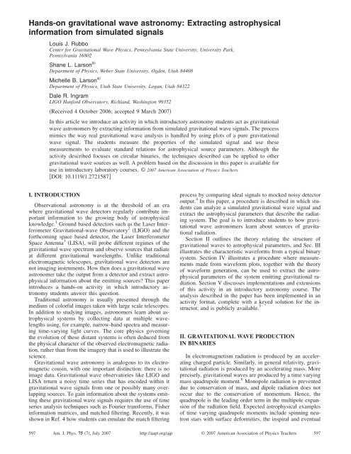
<str<strong>on</strong>g>Hands</str<strong>on</strong>g>-<strong>on</strong> gravitati<strong>on</strong>al <strong>wave</strong> astr<strong>on</strong>omy: Extracting astrophysical<br />
informati<strong>on</strong> from simulated signals<br />
Louis J. Rubbo<br />
Center for Gravitati<strong>on</strong>al Wave <strong>Physics</strong>, Pennsylvania State University, University Park,<br />
Pennsylvania 16802<br />
Shane L. Lars<strong>on</strong> a<br />
<strong>Department</strong> of <strong>Physics</strong>, Weber State University, Ogden, <strong>Utah</strong> 84408<br />
Michelle B. Lars<strong>on</strong> a<br />
<strong>Department</strong> of <strong>Physics</strong>, <strong>Utah</strong> State University, Logan, <strong>Utah</strong> 84322<br />
Dale R. Ingram<br />
LIGO Hanford Observatory, Richland, Washingt<strong>on</strong> 99352<br />
Received 4 October 2006; accepted 9 March 2007<br />
In this article we introduce an activity in which introductory astr<strong>on</strong>omy students act as gravitati<strong>on</strong>al<br />
<strong>wave</strong> astr<strong>on</strong>omers by extracting informati<strong>on</strong> from simulated gravitati<strong>on</strong>al <strong>wave</strong> signals. The process<br />
mimics the way real gravitati<strong>on</strong>al <strong>wave</strong> analysis is handled by using plots of a pure gravitati<strong>on</strong>al<br />
<strong>wave</strong> signal. The students measure the properties of the simulated signal and use these<br />
measurements to evaluate standard relati<strong>on</strong>s for astrophysical source parameters. Although the<br />
activity described focuses <strong>on</strong> circular binaries, the techniques described can be applied to other<br />
gravitati<strong>on</strong>al <strong>wave</strong> sources as well. A problem based <strong>on</strong> the discussi<strong>on</strong> in this paper is available for<br />
use in introductory laboratory courses. © 2007 American Associati<strong>on</strong> of <strong>Physics</strong> Teachers.<br />
DOI: 10.1119/1.2721587<br />
I. INTRODUCTION<br />
Observati<strong>on</strong>al astr<strong>on</strong>omy is at the threshold of an era<br />
where gravitati<strong>on</strong>al <strong>wave</strong> detectors regularly c<strong>on</strong>tribute important<br />
informati<strong>on</strong> to the growing body of astrophysical<br />
knowledge. 1 Ground based detectors such as the Laser Interferometer<br />
Gravitati<strong>on</strong>al-<strong>wave</strong> Observatory 2 LIGO and the<br />
forthcoming space based detector, the Laser Interferometer<br />
Space Antenna 3 LISA, will probe different regimes of the<br />
gravitati<strong>on</strong>al <strong>wave</strong> spectrum and observe sources that radiate<br />
at different gravitati<strong>on</strong>al <strong>wave</strong>lengths. Unlike traditi<strong>on</strong>al<br />
electromagnetic telescopes, gravitati<strong>on</strong>al <strong>wave</strong> detectors are<br />
not imaging instruments. How then does a gravitati<strong>on</strong>al <strong>wave</strong><br />
astr<strong>on</strong>omer take the output from a detector and extract astrophysical<br />
informati<strong>on</strong> about the emitting sources? This paper<br />
introduces a hands-<strong>on</strong> activity in which introductory astr<strong>on</strong>omy<br />
students answer this questi<strong>on</strong>.<br />
Traditi<strong>on</strong>al astr<strong>on</strong>omy is usually presented through the<br />
medium of colorful images taken with large scale telescopes.<br />
In additi<strong>on</strong> to studying images, astr<strong>on</strong>omers learn about astrophysical<br />
systems by collecting data at multiple <strong>wave</strong>lengths<br />
using, for example, narrow-band spectra and measuring<br />
time-varying light curves. The core physics governing<br />
the evoluti<strong>on</strong> of these distant systems is often deduced from<br />
the physical character of the observed electromagnetic radiati<strong>on</strong>,<br />
rather than from the imagery that is used to illustrate the<br />
science.<br />
Gravitati<strong>on</strong>al <strong>wave</strong> astr<strong>on</strong>omy is analogous to its electromagnetic<br />
cousin, with <strong>on</strong>e important distincti<strong>on</strong>: there is no<br />
image data. Gravitati<strong>on</strong>al <strong>wave</strong> observatories like LIGO and<br />
LISA return a noisy time series that has encoded within it<br />
gravitati<strong>on</strong>al <strong>wave</strong> signals from <strong>on</strong>e or possibly many overlapping<br />
sources. To gain informati<strong>on</strong> about the systems emitting<br />
these gravitati<strong>on</strong>al <strong>wave</strong> signals requires the use of time<br />
series analysis techniques such as Fourier transforms, Fisher<br />
informati<strong>on</strong> matrices, and matched filtering. Recently, it was<br />
shown in Ref. 4 how students can emulate the match filtering<br />
process by comparing ideal signals to mocked noisy detector<br />
output. 4 In this paper, a procedure is described in which students<br />
can analyze a simulated gravitati<strong>on</strong>al <strong>wave</strong> signal and<br />
extract the astrophysical parameters that describe the radiating<br />
system. The goal is to introduce students to how gravitati<strong>on</strong>al<br />
<strong>wave</strong> astr<strong>on</strong>omers learn about sources of gravitati<strong>on</strong>al<br />
radiati<strong>on</strong>.<br />
Secti<strong>on</strong> II outlines the theory relating the structure of<br />
gravitati<strong>on</strong>al <strong>wave</strong>s to astrophysical parameters, and Sec. III<br />
illustrates the characteristic <strong>wave</strong>forms from a typical binary<br />
system. Secti<strong>on</strong> IV illustrates a procedure where measurements<br />
made from <strong>wave</strong>form plots, together with the theory<br />
of <strong>wave</strong>form generati<strong>on</strong>, can be used to extract the astrophysical<br />
parameters of the system emitting gravitati<strong>on</strong>al radiati<strong>on</strong>.<br />
Secti<strong>on</strong> V discusses implementati<strong>on</strong>s and extensi<strong>on</strong>s<br />
of this activity in an introductory astr<strong>on</strong>omy course. The<br />
analysis described in the paper has been implemented in an<br />
activity format, complete with a keyed soluti<strong>on</strong> for the instructor,<br />
and is publicly available. 5<br />
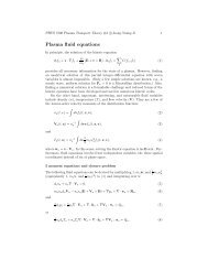
II. GRAVITATIONAL WAVE PRODUCTION<br />
IN BINARIES<br />
In electromagnetism radiati<strong>on</strong> is produced by an accelerating<br />
charged particle. Similarly, in general relativity, gravitati<strong>on</strong>al<br />
radiati<strong>on</strong> is produced by an accelerating mass. More<br />
precisely, gravitati<strong>on</strong>al <strong>wave</strong>s are produced by a time varying<br />
mass quadrupole moment. 6 M<strong>on</strong>opole radiati<strong>on</strong> is prevented<br />
due to c<strong>on</strong>servati<strong>on</strong> of mass, and dipole radiati<strong>on</strong> does not<br />
occur due to the c<strong>on</strong>servati<strong>on</strong> of momentum. Hence, the<br />
quadrupole is the leading order term in the multipole expansi<strong>on</strong><br />
of the radiati<strong>on</strong> field. Expected astrophysical examples<br />
of time varying quadrupole moments include spinning neutr<strong>on</strong><br />
stars with surface deformities, the inspiral and eventual<br />
597 Am. J. Phys. 75 7, July 2007 http://aapt.org/ajp © 2007 American Associati<strong>on</strong> of <strong>Physics</strong> Teachers 597
plunge of compact objects into massive black holes, and P<br />
asymmetric supernovae. 7 orb t = P 8/3 0 − 8 3<br />
This paper focuses <strong>on</strong> an additi<strong>on</strong>al<br />
, 5<br />
example, a binary star system.<br />
where P 0 is the orbital period at time t=0, and k is an evoluti<strong>on</strong><br />
c<strong>on</strong>stant<br />
For a circular binary system, where the comp<strong>on</strong>ents are<br />
treated as point-like particles, the gravitati<strong>on</strong>al <strong>wave</strong>forms<br />
given by<br />
take <strong>on</strong> the seductively simple form<br />
k 96 5/3<br />
<br />
5 c 3 . 6<br />
decrease with time according to 8 depend <strong>on</strong> the chirp mass M and the luminosity distance r, it<br />
ht = Atcos t,<br />
1<br />
As a result of the decreasing orbital period, the two binary<br />
where ht is the gravitati<strong>on</strong>al <strong>wave</strong>form also referred to as<br />
comp<strong>on</strong>ents will slowly inspiral, eventually colliding and<br />
coalescing into a single remnant. For the assumpti<strong>on</strong> of<br />
the gravitati<strong>on</strong>al <strong>wave</strong> strain, At is the time dependent<br />
point-like particles, the coalescence occurs when P<br />
amplitude, and t is the gravitati<strong>on</strong>al <strong>wave</strong> phase. The<br />
orb t=0.<br />
Although gravitati<strong>on</strong>al <strong>wave</strong>s have not yet been detected<br />
amplitude At can be expressed in terms of the parameters directly, they were first indirectly detected through orbital<br />
characterizing the system,<br />
period decay in the early 1970s when Hulse and Taylor observed<br />
the first known binary pulsar, PSR 1913+16.<br />
At = 2GM5/3<br />
2/3<br />
<br />
c 4 , 2<br />
r P gw t<br />
Because<br />
pulsars are extremely accurate clocks, it was possible<br />
to use changes in the pulse intervals to measure the changing<br />
orbital period as the system decays. The orbital decay rate<br />
where G is Newt<strong>on</strong>’s gravitati<strong>on</strong>al c<strong>on</strong>stant, c is the speed of was found to agree with general relativity’s predicti<strong>on</strong> of<br />
light, r is the luminosity distance to the binary, and P gw t is gravitati<strong>on</strong>al radiati<strong>on</strong> to exquisite accuracy. 10<br />
the gravitati<strong>on</strong>al <strong>wave</strong> period. The quantity M It is important to emphasize that Eq. 5 gives the orbital<br />
M 1 M 2 3/5 M 1 +M 2 −1/5 is the chirp mass and appears often<br />
in gravitati<strong>on</strong>al <strong>wave</strong> physics, making it a natural mass<br />
scale. The origin for this nomenclature will become evident<br />
shortly. The gravitati<strong>on</strong>al <strong>wave</strong> phase, t, is analogous to<br />
the phase for other <strong>wave</strong> phenomen<strong>on</strong>. It represents the locati<strong>on</strong><br />
period, not the gravitati<strong>on</strong>al <strong>wave</strong> period. Careful scrutiny of<br />
Eqs. 2 and 3 reveals that the gravitati<strong>on</strong>al <strong>wave</strong> period<br />
P gw t appears in the descripti<strong>on</strong> of the <strong>wave</strong>form. For circularized<br />
binary systems, P orb t and P gw t are simply related<br />
by<br />
of the <strong>wave</strong> cycle which is impinging <strong>on</strong> the detector<br />
at time t, and tracks the evoluti<strong>on</strong> of the <strong>wave</strong>’s amplitude as<br />
P orb t =2P gw t.<br />
7<br />
a functi<strong>on</strong> of time. The phase has units of radians, and is The factor of two stems from the fact that the lowest possible<br />
related to the gravitati<strong>on</strong>al <strong>wave</strong> frequency f gw or, alternatively,<br />
the period P gw = f gw by the integral,<br />
order. Quadrupole moments are invariant under a 180° rota-<br />
order for gravitati<strong>on</strong>al radiati<strong>on</strong> producti<strong>on</strong> is the quadrupole<br />
ti<strong>on</strong>, yielding a factor of two per complete orbit.<br />
t<br />
dt<br />
t = 0 +20 P gw t .<br />
3<br />
III. WAVEFORMS FROM A BINARY SYSTEM<br />
Here 0 is the initial phase value, 0 =t=0.<br />
If we return to the amplitude given in Eq. 2 and substitute<br />
typical values for a neutr<strong>on</strong> star binary located at the<br />
center of our galaxy, we find that gravitati<strong>on</strong>al <strong>wave</strong>s are<br />
As an example of the kind of <strong>wave</strong>forms we expect from<br />
binaries, c<strong>on</strong>sider a binary neutr<strong>on</strong> star system with M 1<br />
=M 2 =1.4M M=1.22M located at the center of the galaxy<br />
r=8 kpc away. We will c<strong>on</strong>sider <strong>wave</strong>forms generated at<br />
extremely weak,<br />
two distinct times in the binary’s evoluti<strong>on</strong>. The first <strong>wave</strong>form<br />
that we will c<strong>on</strong>sider is 10<br />
M r<br />
A =10<br />
1.22 M <br />
5/3<br />
8 kpc<br />
−1 P −2/3<br />
gw<br />
10 s<br />
years before coalescence.<br />
During this phase the gravitati<strong>on</strong>al <strong>wave</strong> frequency is detectable<br />
by the spaceborne LISA observatory, which is sensitive<br />
3 . 4<br />
to radiati<strong>on</strong> between 10 −5 and 1 Hz. The sec<strong>on</strong>d <strong>wave</strong>form<br />
An analysis of the units in Eq. 2 reveals that the amplitude<br />
A is dimensi<strong>on</strong>less. Gravitati<strong>on</strong>al radiati<strong>on</strong> manifests itself in<br />
matter by inducing a strain. In other words, Eq. 1 gives the<br />
relative change in the distance between two points in spacetime<br />
as a functi<strong>on</strong> of time. By m<strong>on</strong>itoring the separati<strong>on</strong><br />
we will c<strong>on</strong>sider is during the final sec<strong>on</strong>d before the neutr<strong>on</strong><br />
star binary coalesces. The gravitati<strong>on</strong>al <strong>wave</strong> frequencies<br />
during this phase are detectable by the terrestrial LIGO observatory,<br />
which is sensitive to gravitati<strong>on</strong>al <strong>wave</strong> frequencies<br />
between 64 and 2000 Hz.<br />
between two or more test masses, it is possible to discern if<br />
a gravitati<strong>on</strong>al <strong>wave</strong> is present. The measurement of the<br />
gravitati<strong>on</strong>al radiati<strong>on</strong> field directly is in c<strong>on</strong>trast to most<br />
electromagnetic observati<strong>on</strong>s where the energy flux the<br />
square of the field is measured.<br />
As in electromagnetism, gravitati<strong>on</strong>al <strong>wave</strong>s have two independent<br />
polarizati<strong>on</strong> states. For a binary system the two<br />
states are related by a 90° phase shift. C<strong>on</strong>sequently, Eq. 1<br />
captures the functi<strong>on</strong>al form for both polarizati<strong>on</strong> states. For<br />
the purposes of this paper <strong>on</strong>ly a single polarizati<strong>on</strong> state and<br />
its associated <strong>wave</strong>form will be discussed.<br />
Gravitati<strong>on</strong>al <strong>wave</strong>s carry energy and angular momentum<br />
away from the binary system causing the orbital period to<br />
A. Far from coalescence<br />
Figure 1 shows the emitted gravitati<strong>on</strong>al radiati<strong>on</strong> l<strong>on</strong>g<br />
before the binary comp<strong>on</strong>ents coalesce. The figure was produced<br />
using Eqs. 1–7 and the values given previously.<br />
During this era of the binary evoluti<strong>on</strong>, the gravitati<strong>on</strong>al<br />
<strong>wave</strong>s are essentially m<strong>on</strong>ochromatic; the orbital period is<br />
evolving too slowly to detect a frequency derivative term.<br />
For such m<strong>on</strong>ochromatic signals the <strong>on</strong>ly measurable properties<br />
of the gravitati<strong>on</strong>al <strong>wave</strong>form are the period P gw and<br />
the orbital period P orb through Eq. 7, the amplitude A, and<br />
the initial phase 0 . Even though the <strong>wave</strong>form equati<strong>on</strong>s<br />
598 Am. J. Phys., Vol. 75, No. 7, July 2007<br />
Rubbo et al. 598
Fig. 1. The gravitati<strong>on</strong>al <strong>wave</strong>form for a binary system c<strong>on</strong>sisting of two<br />
neutr<strong>on</strong> stars far from coalescence and located at the center of our galaxy.<br />
Fig. 3. The chirping <strong>wave</strong>form <strong>on</strong>e sec<strong>on</strong>d before coalescence.<br />
is not possible to solve for their values from the data provided<br />
by the m<strong>on</strong>ochromatic <strong>wave</strong>form. Not enough informati<strong>on</strong><br />
exists to completely solve Eqs. 2 and 5 for both<br />
quantities. The inability to detect a change in the orbital period<br />
can be seen by c<strong>on</strong>sidering the relative size of the two<br />
terms in Eq. 5. If we use the binary neutr<strong>on</strong> star chirp mass<br />
M=1.22 M , it is evident that the sec<strong>on</strong>d term is negligible<br />
compared to the period P 0 of the <strong>wave</strong> shown in Fig. 1. In<br />
the parlance of gravitati<strong>on</strong>al <strong>wave</strong> astr<strong>on</strong>omy, there is a<br />
mass-distance degeneracy in the <strong>wave</strong>form descripti<strong>on</strong>,<br />
analogous to the familiar mass-inclinati<strong>on</strong> degeneracy in the<br />
electromagnetic observati<strong>on</strong>s of spectroscopic binaries. 11<br />
This degeneracy is well known, but we will show that it can<br />
be broken if the orbital period of the binary evolves during<br />
the gravitati<strong>on</strong>al <strong>wave</strong> observati<strong>on</strong>s.<br />
B. Near coalescence<br />
Inspecti<strong>on</strong> of Eq. 5 shows that, as time goes <strong>on</strong>, the<br />
emissi<strong>on</strong> of gravitati<strong>on</strong>al <strong>wave</strong>s causes the orbital period to<br />
become shorter and, as a result, the frequency of the emitted<br />
<strong>wave</strong>s increases. Similarly, c<strong>on</strong>siderati<strong>on</strong> of Eq. 2 shows<br />
that as the <strong>wave</strong> period decreases, the time dependent amplitude<br />
At increases. These changes are characteristic of<br />
gravitati<strong>on</strong>al <strong>wave</strong>s emitted just prior to a source coalescence<br />
and are referred to collectively as a chirp signal. The chirp<br />
<strong>wave</strong>form emitted by the example binary neutr<strong>on</strong> star system<br />
just prior to coalescence is illustrated in Fig. 2.<br />
A binary signal that evolves appreciably during the gravitati<strong>on</strong>al<br />
<strong>wave</strong> observati<strong>on</strong> is called a chirping binary. In these<br />
cases, the mass parameter M which appears in the amplitude<br />
At and in the period evoluti<strong>on</strong> c<strong>on</strong>stant k can be determined<br />
from measurements of the evolving signal. For this<br />
reas<strong>on</strong>, the mass M is called the chirp mass. To leading<br />
order in the gravitati<strong>on</strong>al <strong>wave</strong> producti<strong>on</strong>, it is not possible<br />
to measure the individual masses, <strong>on</strong>ly the chirp mass. C<strong>on</strong>sequently,<br />
it is not possible to distinguish between binaries<br />
with the same chirp mass. For example, the binary neutr<strong>on</strong><br />
star c<strong>on</strong>sidered here with M 1 =M 2 =1.4 M has roughly the<br />
same chirp mass as a binary with an M 1 =10 M black hole<br />
and a M 2 =0.3 M white dwarf.<br />
To extract the chirp mass from measurements of the gravitati<strong>on</strong>al<br />
<strong>wave</strong>form, c<strong>on</strong>sider two small stretches of the chirping<br />
<strong>wave</strong>form. Figure 3 shows the <strong>wave</strong>form from 0 st<br />
0.05 s, and Fig. 4 shows the <strong>wave</strong>form from 0.9 st<br />
0.92 s. The <strong>wave</strong>form is appreciably different between<br />
these two snapshots, both in amplitude At and in period<br />
P gw t. This difference allows the degeneracy found in the<br />
m<strong>on</strong>ochromatic signal case to be broken, because the gravitati<strong>on</strong>al<br />
<strong>wave</strong> period can be measured at two different times<br />
and used in Eq. 5 to solve for the chirp mass M.<br />
IV. MEASURING GRAVITATIONAL WAVEFORMS<br />
This secti<strong>on</strong> illustrates a procedure where introductory astr<strong>on</strong>omy<br />
students can make measurements from the figures<br />
in Sec. III using a straight edge. From their measured data<br />
Fig. 2. The <strong>wave</strong>form over the last sec<strong>on</strong>d before coalescence. Because the<br />
signal’s amplitude and frequency increase with time, these types of systems<br />
are said to be chirping.<br />
Fig. 4. The chirping <strong>wave</strong>form <strong>on</strong>e-tenth of a sec<strong>on</strong>d before coalescence.<br />
599 Am. J. Phys., Vol. 75, No. 7, July 2007<br />
Rubbo et al. 599
and the theoretical results in Sec. II they can deduce the<br />
astrophysical character of the system emitting the gravitati<strong>on</strong>al<br />
<strong>wave</strong>forms.<br />
A. M<strong>on</strong>ochromatic <strong>wave</strong>forms<br />
Limited astrophysical informati<strong>on</strong> can be extracted directly<br />
from Fig. 1, as will be the case with true m<strong>on</strong>ochromatic<br />
signals detected by gravitati<strong>on</strong>al <strong>wave</strong> observatories.<br />
With limited assumpti<strong>on</strong>s more detailed informati<strong>on</strong> can be<br />
deduced. A suitable extracti<strong>on</strong> and analysis procedure for an<br />
introductory astr<strong>on</strong>omy student would proceed in the following<br />
manner:<br />
1 Measure the gravitati<strong>on</strong>al <strong>wave</strong> period P gw from Fig. 1.<br />
Because the signal is m<strong>on</strong>ochromatic and the binary is<br />
circular, the orbital period P orb is obtained from P gw using<br />
Eq. 7. For the <strong>wave</strong>form in Fig. 1, a careful measurement<br />
should yield P gw =1000 s.<br />
2 Measure the maximum value for ht shown in Fig. 1.<br />
This is the value for the amplitude A given in Eq. 2.As<br />
noted in Sec. III A, no astrophysical informati<strong>on</strong> can be<br />
extracted from the amplitude al<strong>on</strong>e. When a binary system<br />
is far from coalescence, it is not possible to detect a<br />
changing orbital period. From Eq. 2 the same can be<br />
said about the amplitude. Therefore, the amplitude measured<br />
here can be taken to be time-independent.<br />
3 Measure the initial phase for the <strong>wave</strong>form displayed in<br />
Fig. 1. This is d<strong>on</strong>e by noting that at t=0 the gravitati<strong>on</strong>al<br />
<strong>wave</strong>form reduces to<br />
ht =0 = A cos 0 ,<br />
8<br />
which in turn implies that<br />
ht =0<br />
0 = cos−1 . 9<br />
A<br />
For the plots in Fig. 1, a careful measurement should<br />
give a value near 0 =/70.45. The initial phase does<br />
not represent an intrinsic property of the binary; its value<br />
is a c<strong>on</strong>sequence of when the gravitati<strong>on</strong>al <strong>wave</strong> observati<strong>on</strong>s<br />
began. To illustrate this property of the initial<br />
phase, imagine relabeling the time axis in Fig. 1 to represent<br />
a new observati<strong>on</strong> that started later than the observati<strong>on</strong><br />
shown. The initial phase will have a new value,<br />
but the <strong>wave</strong>form does not change because the intrinsic<br />
properties of the binary did not change.<br />
4 If a gravitati<strong>on</strong>al <strong>wave</strong> astr<strong>on</strong>omer were to assume that<br />
the binary was a pair of neutr<strong>on</strong> stars, the comp<strong>on</strong>ent<br />
mass values could be assigned as part of the assumpti<strong>on</strong>.<br />
Most neutr<strong>on</strong> star masses cluster around M =1.4 M .A<br />
good initial assumpti<strong>on</strong>, and <strong>on</strong>e that we will make from<br />
this point <strong>on</strong>, is that each comp<strong>on</strong>ent of the binary has<br />
this mass. As noted in Sec. III A, this assumpti<strong>on</strong> can be<br />
dangerous because similar chirp masses, M, can result<br />
from significantly different systems. Additi<strong>on</strong>al informati<strong>on</strong><br />
not present in the gravitati<strong>on</strong>al <strong>wave</strong>form might help<br />
an astr<strong>on</strong>omer be more c<strong>on</strong>fident about such an assumpti<strong>on</strong>.<br />
For example, an associated simultaneous electromagnetic<br />
signal or the locati<strong>on</strong> of the source <strong>on</strong> the sky<br />
may favor <strong>on</strong>e model of the binary over another. With<br />
the assumed comp<strong>on</strong>ent masses, the orbital separati<strong>on</strong> R<br />
of the binary comp<strong>on</strong>ents can be computed from the<br />
measured orbital period by using Kepler’s third law,<br />
Gm 1 + m 2 = 2 2<br />
P orb R 3 .<br />
10<br />
For this example, the orbital separati<strong>on</strong> is R=1.4<br />
10 −3 AU=2.110 8 m, a little less than the separati<strong>on</strong><br />
of the Earth and the Mo<strong>on</strong>.<br />
5 If the masses are assumed, the distance to the binary can<br />
be calculated from Eq. 2 and the measured amplitude.<br />
If careful measurements have been made, the answer<br />
should be close to the value r=8 kpc=2.510 20 m.<br />
6 Finally, if the masses are assumed, it can be shown that<br />
the m<strong>on</strong>ochromatic descripti<strong>on</strong> is a good <strong>on</strong>e for this<br />
<strong>wave</strong> by computing the value of the sec<strong>on</strong>d term in Eq.<br />
5 and showing that it is negligible compared to the<br />
measured period P 0 . The sec<strong>on</strong>d term in Eq. 5 is found<br />
by using the assumed mass values to get the chirp mass<br />
and the final time shown <strong>on</strong> the plot for the value of t.<br />
B. Chirping <strong>wave</strong>forms<br />
For a chirping <strong>wave</strong>form, additi<strong>on</strong>al astrophysical informati<strong>on</strong><br />
associated with the system can be extracted directly<br />
from measurements of the <strong>wave</strong>form without making underlying<br />
assumpti<strong>on</strong>s like those needed when the system is far<br />
from coalescence. To extract informati<strong>on</strong> from the chirping<br />
<strong>wave</strong>form shown in Fig. 2, the two zoom-ins of the <strong>wave</strong>form<br />
shown in Figs. 3 and 4 will be used. A typical extracti<strong>on</strong><br />
procedure might look like the following:<br />
1 For Figs. 3 and 4, measure the period of <strong>on</strong>e cycle of the<br />
<strong>wave</strong> and note the time, t, at which the periods were<br />
measured. The amplitudes At should be measured for<br />
the same cycle as the periods.<br />
2 If the period measured at time t 1 in Fig. 3 is P 0 , and the<br />
period measured at time t 2 in Fig. 4 is P gw t at time t<br />
=t 2 −t 1 , then Eq. 5 can be used to deduce the chirp<br />
mass, M, of the system.<br />
3 Once the chirp mass M has been determined, the distance<br />
to the binary can be computed by using Eq. 2<br />
with the measured amplitude At and period P gw t of<br />
each <strong>wave</strong>form. The results from the two figures can be<br />
averaged together to obtain a final result for the distance<br />
to the binary.<br />
V. DISCUSSION<br />
The activity described here introduces how gravitati<strong>on</strong>al<br />
<strong>wave</strong> astr<strong>on</strong>omers extract astrophysical informati<strong>on</strong> from observed<br />
binary <strong>wave</strong>forms. Real signal analysis is more complex.<br />
The most significant challenge for real data analysis is<br />
identifying the signal buried in a noisy data stream. A comm<strong>on</strong><br />
approach to this problem in gravitati<strong>on</strong>al <strong>wave</strong> astr<strong>on</strong>omy<br />
is to use template matching, which has been explored<br />
in a separate activity. 4 If a signal is present in a noisy<br />
data stream, the template provides a way to subtract the noise<br />
and leave a clean <strong>wave</strong>form. This activity assumes a signal<br />
template has been selected. Astr<strong>on</strong>omers estimate the values<br />
of astrophysical parameters describing a source of gravitati<strong>on</strong>al<br />
<strong>wave</strong>s from clean <strong>wave</strong>forms.<br />
We have introduced the core calculati<strong>on</strong>s in gravitati<strong>on</strong>al<br />
<strong>wave</strong> astrophysics that an introductory astr<strong>on</strong>omy student<br />
can perform in a laboratory setting to gain informati<strong>on</strong> about<br />
600 Am. J. Phys., Vol. 75, No. 7, July 2007<br />
Rubbo et al. 600
an astrophysical system. To complement this article we have<br />
developed a detailed student activity sheet and corresp<strong>on</strong>ding<br />
teacher’s guide in Sec. IV. The complementary material is<br />
available at Ref. 5.<br />
ACKNOWLEDGMENTS<br />
This work was supported by the Center for Gravitati<strong>on</strong>al<br />
Wave <strong>Physics</strong>, which is funded by the Nati<strong>on</strong>al Science<br />
Foundati<strong>on</strong> under cooperative agreement PHY-01-14375.<br />
The authors would like to thank the LIGO Laboratory. The<br />
LIGO Observatories were c<strong>on</strong>structed by the California Institute<br />
of Technology and Massachusetts Institute of Technology<br />
with funding from the Nati<strong>on</strong>al Science Foundati<strong>on</strong> under<br />
cooperative agreement PHY-9210038. The LIGO<br />
Laboratory operates under cooperative agreement PHY-<br />
0107417. This paper has been assigned LIGO Document<br />
Number LIGO-P060064-00-Z.<br />
a Formerly at the Center for Gravitati<strong>on</strong>al Wave <strong>Physics</strong>, Pennsylvania<br />
State University, University Park, Pennsylvania 16802.<br />
1 L. J. Rubbo, S. L. Lars<strong>on</strong>, M. B. Lars<strong>on</strong>, and K. D. Zaleski, “Gravitati<strong>on</strong>al<br />
<strong>wave</strong>s: New observatories for new astr<strong>on</strong>omy,” Phys. Teach. 44,<br />
420–423 2006.<br />
2 A. Abramovici et al., “LIGO: The laser interferometer gravitati<strong>on</strong>al-<strong>wave</strong><br />
observatory,” Science 256, 325–333 1992.<br />
3 T. J. Sumner and D. N. A. Shaul, “The observati<strong>on</strong>s of gravitati<strong>on</strong>al<br />
<strong>wave</strong>s from space using LISA,” Mod. Phys. Lett. A 19, 785–800 2004.<br />
4 M. B. Lars<strong>on</strong>, L. J. Rubbo, K. D. Zaleski, and S. L. Lars<strong>on</strong>, “Science<br />
icebreaker activities: An example from gravitati<strong>on</strong>al <strong>wave</strong> astr<strong>on</strong>omy,”<br />
Phys. Teach. 44, 416–419. 2006.<br />
5 cgwp.gravity.psu.edu/outreach/activities/.<br />
6 B. F. Schutz, “Gravitati<strong>on</strong>al <strong>wave</strong>s <strong>on</strong> the back of an envelope,” Am. J.<br />
Phys. 52, 412–419 1984.<br />
7 C. Cutler and K. S. Thorne, “An overview of gravitati<strong>on</strong>al-<strong>wave</strong><br />
sources,” in General Relativity and Gravitati<strong>on</strong>: Proceedings of the 16th<br />
Internati<strong>on</strong>al C<strong>on</strong>ference, edited by N. T. Bishop and S. D. Maharaj<br />
World Scientific, 2002, p.72.<br />
8 J. B. Hartle, Gravity: An Introducti<strong>on</strong> to Einstein’s General Relativity<br />
Addis<strong>on</strong>-Wesley, San Francisco, 2003, p. 508.<br />
9 R. A. Hulse, “The discovery of the binary pulsar,” Rev. Mod. Phys. 66,<br />
699–710 1994.<br />
10 J. H. Taylor Jr., “Binary pulsars and relativistic gravity,” Rev. Mod. Phys.<br />
66, 711–719 1994.<br />
11 B. W. Carroll and D. A. Ostlie, An Introducti<strong>on</strong> to Modern Astrophysics<br />
Addis<strong>on</strong>-Wesley, San Francisco, 2007, 2nd ed., Chap. 7.<br />
601 Am. J. Phys., Vol. 75, No. 7, July 2007<br />
Rubbo et al. 601