Solution to problem set 4

Microeconomics B01.1303
Prof. N. Economides
Solutions to problem set 4
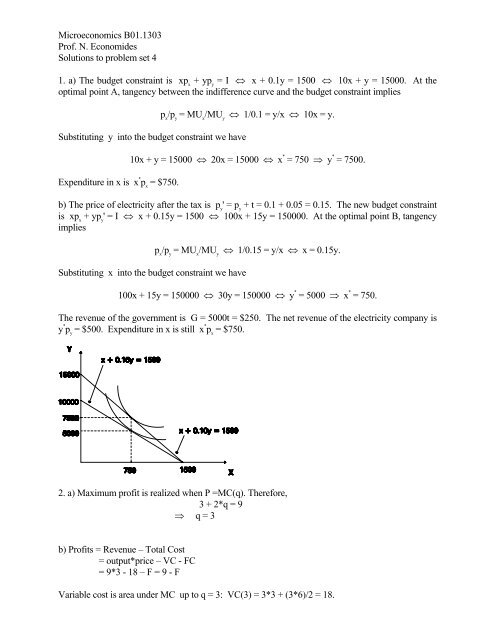
1. a) The budget constraint is xp x
+ yp y
= I ⇔ x + 0.1y = 1500 ⇔ 10x + y = 15000. At the
optimal point A, tangency between the indifference curve and the budget constraint implies
Substituting y into the budget constraint we have
Expenditure in x is x * p x
= $750.
p x
/p y
= MU x
/MU y
⇔ 1/0.1 = y/x ⇔ 10x = y.
10x + y = 15000 ⇔ 20x = 15000 ⇔ x * = 750 ⇒ y * = 7500.
b) The price of electricity after the tax is p y
' = p y
+ t = 0.1 + 0.05 = 0.15. The new budget constraint
is xp x
+ yp y
' = I ⇔ x + 0.15y = 1500 ⇔ 100x + 15y = 150000. At the optimal point B, tangency
implies
Substituting x into the budget constraint we have
p x
/p y
= MU x
/MU y
⇔ 1/0.15 = y/x ⇔ x = 0.15y.
100x + 15y = 150000 ⇔ 30y = 150000 ⇔ y * = 5000 ⇒ x * = 750.
The revenue of the government is G = 5000t = $250. The net revenue of the electricity company is
y * p y
= $500. Expenditure in x is still x * p x
= $750.
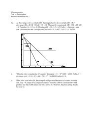
2. a) Maximum profit is realized when P =MC(q). Therefore,
3 + 2*q = 9
⇒ q = 3
b) Profits = Revenue – Total Cost
= output*price – VC - FC
= 9*3 - 18 – F = 9 - F
Variable cost is area under MC up to q = 3: VC(3) = 3*3 + (3*6)/2 = 18.

We don’t have enough information on how large is the fixed cost, so we assume it is F.
Price, MC(q)
27
24
21
18
MC(q) = 3 + 2q
15
12
9
Profits = 9
P = 9
6
3
Variable Cost = 18
0
0 1 2 3 4 5 6 7 8 9 10
Output
3.
a) TC = Q 2 + 100, MC = 2Q, AVC = Q, ATC = Q + 100/Q.
b) Short run supply curve is equal to MC for all prices because MC is greater than AVC for all
prices. Long run supply curve is equal to MC for all prices above $20. This is the price at which
MC>ATC. See graph. For all prices below $20, the long run supply curve will be along the Y-axis
(no wheat will be supplied).
c) P = MR = MC
25 = 2Q ⇒ Q = 12.5
Profit = P*Q - TC = 25*12.5 - 12.5 2 - 100 = 56.25
d) TC = 25Q, MC = 25, AVC = 25, ATC = 25

For prices < $25, the farmer will not supply anything to the market because he will lose
money in the short and long run.
For prices > $25, he will supply as much as he possibly can because he makes a profit on
each unit he supplies.
e) He will use the new technology for all prices above $25. For all prices above $25, he can make an
“infinite” profit under the new technology. For prices below $20 he would choose not to supply any
wheat. For prices between $20 and $25, he would lose money with the new technology and make
money with the old; therefore for these prices he will use the old technology.