biologia - Studia

BIOLOGIA 

1/2010

ANUL LV 2010 

S T U D I A 

UNIVERSITATIS BABEŞ-BOLYAI 

BIOLOGIA 

1 

Desktop Editing Office: 51 ST B.P. Hasdeu, Cluj-Napoca, Romania, Phone + 40 264-40.53.52 

CUPRINS – CONTENT – SOMMAIRE – INHALT 

L. PÂRVULESCU, Comparative Biometric Study of Crayfish Populations in 

the Anina Mountains (SW Romania) Hydrographic Basins............................... 3 

M. MANU, Structure and Dynamics of Predator Mite Populations (Acari- 

Mesostigmata) in Shrub Ecosystems in Prahova and Doftana Valleys ............ 17 

A. CRIŞAN, Leaf-Beetles (Coleoptera, Chrysomelidae) from the Area BistriŃa 

Bârgăului- ColibiŃa- Piatra Fântânele, a Part of “Nature 2000” Cuşma Site 

(NE Romania)................................................................................................... 31 

A. KONTER, Platform Initiation, Clutch Initiation and Clutch Size in Colonial 

Great Crested Grebes (Podiceps cristatus) .................................................... 45 

M. R. MOLAEI, A Mathematical Model for an Epidemic in an Open Society ..... 61 

O. RABIEI MOTLAGH, Z. AFSHARNEZHAD, On the Conditions for which 

the Atm Protein Can Switch Off the DNA Damage Signal in a p53 Model. .. 67 

V. BERCEA, C. COMAN, N. DRAGOŞ, The Inducement of Chlorophyll 

Fluorescence in State Transitions under Low Temperature in the Mougeotia 

Alga, Strain AICB 560.........................................................................................81 

R. TÖRÖK-OANCE, V. NICULESCU, M. N. FILIMON, Modification of the 

Bone Mineral Density, T-Score and Z-Score Values According to Age and 

Anatomic Region in Osteoporosis Cases…………….…………………..........91

Ş.-C. MIRESCU, L. CIOBANU, V. ANDREICA, C.-L. ROŞIORU, The 

Electrical Resistance of Acupuncture Source Points as a Relevant Factor for 

Inner Organ Status………………………………………………… ...............103 

M. C. ALUPEI, R. M. MAXIM, M. BANCIU, Oxidative Stress and Inflammation - 

Key Players in Tumor Angiogenesis……………......................................... 111 

M. DRĂGAN-BULARDA, R. CARPA, M. MIŞCA, V. CĂLEAN, Obtaining 

and Characterization of an α-Amylase by a Strain of Bacillus subtilis…….. 119 

V. MUNTEAN, C.-G. MAIER, R. CARPA, C. MUREŞAN, A. C. FARKAS, 

Microbiological and Enzymological Study on Sediments and Water of the 

River Someşul Mic Upstream the Gilău (Cluj County) Treatment Plant….....131 

All authors are responsible for submitting manuscripts in comprehensible 

US or UK English and ensuring scientific accuracy. 

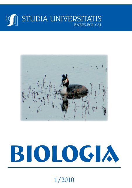
Original picture on front cover © Alin David

STUDIA UNIVERSITATIS BABEŞ – BOLYAI, BIOLOGIA, LV, 1, 2010, p. 3-15 

COMPARATIVE BIOMETRIC STUDY OF CRAYFISH 

POPULATIONS IN THE ANINA MOUNTAINS (SW ROMANIA) 

HYDROGRAPHIC BASINS 

LUCIAN PÂRVULESCU 1 

SUMMARY. The paper presents data concerning the biometric aspects of 

two crayfish species from the rivers of the Anina Mts: the stone crayfish 

(Austropotamobius torrentium) and the noble crayfish (Astacus astacus). 

The populations of the two species are not evenly distributed within the 

three hydrographic basins of the investigated area: Bârzava, Caraş, and Nera. 

Thus, through the discriminant analysis of the measured parameters we were 

able to identify several parameters that proved to be highly related to the 

differentiation of the studied specimens into hydrographic basins; these 

specimens have been afterwards the subject of the ANOVA type analysis. 

The study revealed that, whereas the A. torrentium populations from the Caraş 

basin present high significantly differences in comparison to the populations 

analysed in the Nera basin, the A. astacus populations from the Caraş basin 

differ significantly from those of the Bârzava basin. As far as the morphometric 

differences between the two sexes are concerned, the most powerful and 

visible distinctions that have been registered for both species can be found at 

the level of chela, propodus length, dactylus length and width of chela. The 

maximum dimension of the A. torrentium males, as well as the average of 

these values, is very close to the female one, while for the A. astacus the 

differences between the sexes are much more significant. 

Keywords: Anina Mountains, Astacus astacus, Austropotamobius torrentium, 

biometry, populations 

Introduction 

Freshwater crayfish residing in the Romanian aquatic ecosystems belong to 

the Decapoda orders; they are represented by three indigenous species and an 

invasive one (Pârvulescu, 2009c). Among these, two indigenous species are present 

in the Anina Mountains: Austropotamobius torrentium (Schrank 1803) and Astacus 

astacus (Linnaeus 1758) (Pârvulescu 2009a). The main purpose of the comparative 

study regarding the biometry of different populations is to point out the morphological 

1 West University of Timisoara, Faculty of Chemistry, Biology, Geography, Dept. of Biology, 16A Pestalozzi 

St., 300115, Timisoara; e-mail: parvulescubio@cbg.uvt.ro

L. PÂRVULESCU 

similarities and dissimilarities between populations that are geographically 

separated into different hydrographic basins, as a result of diverse environmental 

influences (Ďuriš et al., 2006; Burba et al., 1999; Papadopol and Diaconu, 1987; 

Gutiérrez-Yurrita et al., 1996; Streissl and Hödl, 2002). Studies regarding the three 

indigenous species of crayfish in Romania have also been published by Papadopol 

and Diaconu, in 1987. 

The investigated area, i.e. the Anina Mountains, is located in southwestern 

Romania; it has a surface of 770 km 2 (Sencu, 1978) most of which is included in 

two National Parks: Semenic-Cheile Caraşului (Semenic – Caras Gorges) National 

Park and Cheile Nerei-BeuşniŃa (Nera Gorges - Beusnita) National Park. The area 

of these mountains gathers three hydrographic basins: Bârzava, Caraş and Nera, 

basins that collect both surface water and ground water. The Caraş and the Nera 

rivers are the direct tributaries of the Danube River, and the Bârzava River flows 

into the Danube River, after the confluence with the Timiş River (Ujvari, 1972). 

The A. astacus species lives almost exclusively in the Caraş basin, with the 

exception of the Buhui stream and the Cândeni River. The Nera basin shows 

exclusively the presence of the species A. torrentium, while the Bârzava basin 

displays a mixture of populations from both species that can be found in different 

streams. (Pârvulescu, 2009a). 

Taking into consideration the quality of the aquatic habitats, the Bârzava 

basin is affected by a powerful anthropic impact; on its upper stream there are three 

artificial dams and various villages which clearly affect the water quality and, 

implicitly, the quality of the aquatic fauna. The upper stream of the Caraş River 

presents a very low anthropic impact and registers a very high water quality, with few 

punctiform exceptions. In the Nera Basin the anthropic impact is scattered along the 

small villages situated on the stream of the rank 1 tributaries and that alter the 

water quality, like in the case of the Cândeni creek, where almost an entire 

popuation was destroyed as a result of the usage of modern detergents within a 

traditional wash house. (Pârvulescu, 2009b). 

Materials and Methods 

The biologic samples were collected in August 2008 and June - July 2009, 

in a total of 52 sampling stations, on all the permanent waters in the upper sector of 

the Bârzava, Caraş and Nera rivers. Each sampling station comprised at least 200 

m of the river under investigation, with similar catching effort. The crayfish were 

collected using active methods, i.e. direct hand sampling from the waterbed, by 

checking the galleries within banks and the spaces between roots or rocks. 

4

BIOMETRIC STUDY OF CRAYFISH POPULATIONS IN THE ANINA MOUNTAINS 

Fig. 1. The biometric parameters measured during the biometric studies 

for the crayfish from the Anina Mountains 

5


The crayfish were identified in situ according to their morphological features, 

sexed and measured. Subsequently, the specimens were set free exactly in the same 

location where they had been captured. We have labeled as population all the 

specimens belonging to one species within each of the three hydrographic basins. For 

the biometric measurements we have used an electronic Black and Decker caliper with 

the maximum width of 150 mm and an accuracy of 0.01 mm. The measured 

parameters (see figure 1) are only those distances which allow the firm grip of the 

measuring tool. The morphological characteristics measured were: TL – total body 

length, CTL - cephalothorax (shell) length, mTW - maximum thoracic (shell) width, 

RL - rostrum length (for the value that indicates the length of the rostrum we subtracted 

from the value of the cephalothorax length (CTL) the value of the post-orbital 

cephalothorax length), 2AW – second abdominal segment width, TW – width of 

telson, PL – propodus length, DL – dactylus length and CW – width of chela. We have 

measured only the specimens that did not present any sign that both chelae have been 

regenerated. All specimens have been measured by the same person. The specimens 

that were smaller than 50 mm total body length have not been measured. 

In order to show which of the measured parameters are relevant for the 

morphological differences, we have processed the data with the help of the 

discriminant analysis, a technique used to classify cases into categorical-dependent 

values that helps us obtain pairs of parameters that are significantly different within 

the lot of the measured data. The means, the standard deviations, the minimum and 

the maximum as well as the ANOVA tests have also been measured. In order to do 

this statistical analysis and to create the diagrams, we used the Statistica StatSoft 

Inc. software (version 7.00 for Windows). 

6 

Results 

During the investigations performed in the summers of 2008 and 2009 in 

the rivers of the Anina Mountains, 115 specimens from the A. torrentium species 

and 73 specimens from the A. astacus species have been measured. The species are 

not evenly distributed in all the three hydrographic basins, according to the already 

published data (Pârvulescu, 2009a). Thus, for the A. torrentium species the most 

representative streams have been the streams of the Nera basin. The species was 

also found in the Caraş and Bârzava basins. As far as the A. astacus species is 

concerned, the most representative have been the streams from the Caraş basin. 

The species was also found in the Bârzava basin, especially in the reservoirs. The 

biometric data have been summarized in Tables 1 and 2. 

According to the data from Tables 1 and 2, we can notice that the clearest 

differences between the sexes are represented by the dimensions of the chelae. 

However, we cannot use this difference alone if we are to correctly make a distinction 

between the sexes. Many and diverse situations may appear in nature when the chela 

may be abnormally well-developed: regeneration after breakage, malformations etc 

(Pârvulescu et al., 2009).


Table 1. 

Biometric data (mm) for the A. torrentium species, measured during the summer 

campaign of 2008-2009, in the Anina Mts. (N = number of specimens). 

Austropotamobius torrentium 

Male (N=57) 

Female (N=58) 

Parameter Min * -Max Mean ± SD Min * -Max Mean ± SD 

TL 50.0-94.0 69.07 ± 10.862 50.53-93.34 67.16 ± 10.403 

CTL 23.7-48.9 34.5 ± 6.01 24.6-44.37 31.46 ± 5.512 

RL 4.8-9.1 6.78 ± 1.072 4.78-9.6 6.66 ± 1.057 

mTW 11.78-27.9 18.72 ± 3.76 12.3-24.02 17.04 ± 2.907 

2AW 6.17-20.9 15.33 ± 2.737 11.5-25.43 16.97 ± 3.486 

TW 5.9-13.7 9.42 ± 1.789 5.93-14.1 9.37 ± 1.884 

PL 16.6-49.9 29.95 ± 8.021 15.79-33.56 22.59 ± 4.578 

DL 10.08-28.5 17.23 ± 4.75 8.91-20.45 13.21 ± 2.757 

CW 7.8-19.6 13.05 ± 3.235 6.75-13.2 10.05 ± 2.036 

Sex ratio 1:1.017 

* Specimens smaller than 50 mm in total length have not been measured 

Biometric data for the (mm) A. astacus species, measured during the summer 

campaign 2008-2009, in the Anina Mts. (N = number of specimens). 

Table 2. 

Astacus astacus 

Male (N=39) 

Female (N=34) 

Parameter Min * -Max Mean ± SD Min * -Max Mean ± SD 

TL 61.34-127.34 99.73 ± 17.978 55.85-108.8 86.8 ± 14.543 

CTL 27.06-68.46 51.46 ± 10.878 27.82-54.07 42.98 ± 8.022 

RL 5.21-18.8 12.1 ± 2.671 6.45-12.6 10.49 ± 1.779 

mTW 15.45-49.97 28.82 ± 7.621 14.42-29.31 23.24 ± 4.63 

2AW 13.17-31.09 22.93 ± 4.31 12.34-28.26 21.97 ± 4.655 

TW 7.34-18.14 13.23 ± 2.414 6.83-14.7 11.38 ± 2.278 

PL 20.65-85.5 47.79 ± 16.925 18.92-42.7 32.22 ± 8.13 

DL 11.69-48.36 28.08 ± 10.181 10.99-25.6 19.2 ± 4.778 

CW 9.13-32.67 20.53 ± 6.555 8.19-20.5 14.43 ± 3.708 

Sex ratio 1:0.871 

* Specimens smaller than 50 mm in total length have not been measured 

In order to compare the populations we have resorted to the discriminant 

analysis that allows to find the most powerful correlated sets of values that could 

differentiate the specimens from different hydrographic basins. Thus, the correlation 

7


matrix for the A. torrentium (Table 3) shows that the most powerful discriminative 

character is represented by the groups of values propodus length – dactylus length (PL- 

DL), propodus length – width of chela (PL-CW) and dactylus length – width of chela 

(DL-CW). 

Table 3. 

Correlation matrix between the measured parameters for the 

A. torrentium specimens in the Anina Mts. in 2008-2009. 

correl. TL CTL RL mTW 2AW TW PL DL CW 

TL 1.00 

CTL 0.91 1.00 

RL 0.82 0.81 1.00 

mTW 0.95 0.94 0.81 1.00 

2AW 0.84 0.73 0.71 0.76 1.00 

TW 0.75 0.70 0.82 0.73 0.68 1.00 

PL 0.83 0.89 0.73 0.92 0.55 0.62 1.00 

DL 0.82 0.88 0.76 0.90 0.56 0.65 0.98 1.00 

CW 0.82 0.87 0.72 0.90 0.56 0.62 0.97 0.95 1.00 

The correlation matrix for the A. astacus (Table 4) shows that the most 

powerful discriminative character is represented by the same groups of values that 

are relevant for the previous species and by the total length – cephalothorax length 

(TL-CTL). 

Table 4. 

Correlation matrix between the parameters measured for the A. astacus 

specimens in the Anina Mts. in 2008-2009. 

correl. TL CTL RL mTW 2AW TW PL DL CW 

TL 1.00 

CTL 0.97 1.00 

RL 0.89 0.89 1.00 

mTW 0.92 0.93 0.84 1.00 

2AW 0.92 0.86 0.78 0.82 1.00 

TW 0.80 0.76 0.76 0.72 0.73 1.00 

PL 0.92 0.92 0.83 0.88 0.77 0.72 1.00 

DL 0.91 0.92 0.83 0.86 0.76 0.73 0.98 1.00 

CW 0.90 0.90 0.80 0.85 0.77 0.69 0.97 0.96 1.00 

8


In our studies, for the comparison of these populations, we have used ratio 

among these parameters. Therefore, for both species we have measured the proportion 

between propodus and dactylus length, propodus length and chela width, dactylus 

length and chela width and also total length and cephalothorax length (table 5). 

Table 5. 

Rapports that show a discriminative character for the crayfish specimens measured 

in the Anina Mts. 

Austropotamobius torrentium 

Astacus astacus 

Ratio between 

Abbreviation Ratio between 

Abbreviation 

parameters: 

parameters: 

- - TL and CTL TL/CTL 

PL and DL PL/DL PL and DL PL/DL 

PL and CW PL/CW PL and CW PL/CW 

DL and CW DL/CW DL and CW DL/CW 

For our comparison between different populations we have used the 

ANOVA test, in order to underline the differences between specimens of the same 

sex, from different hydrographic basins. The individuals of A. torrentium species, 

that inhabit mainly the Nera basin, have also been found well represented in high 

number of individuals in two streams of the Caraş basin and in five streams of the 

Bârzava basin. According to the analysis of the diagrams from Figures 2 A, B and 

C the female populations of crayfish within the three investigated basins are not 

significantly different. However, we may notice a greater resemblance between the 

populations of the Nera and of the Bârzava basins. 

For A. torrentium species the males have been captured in a rather small 

number of specimens in the Bârzava basin; that is why, for the data analysis only the 

specimens captured in the Nera and Caraş basins have been taken into account. They 

display statistically significant differences in the case of the ratio PL/CW (p=0.01971) 

(Fig. 3). 

The A. astacus species was found in the Anina Mountains only in the Caras 

and Bârzava basins; in the upper part of the Bârzava River the species was 

discovered especially in reservoirs. After analyzing the distinct diagrams for the 

two sexes, we can state that the female populations from the two investigated 

basins are significantly different concerning the ratio between propodus length and 

chela width, as well as between dactylus length and chela width (Figs 4 A and B). 

9


1,80 

F(2, 55)=0.42758, p=0.65424 

Vertical bars denote 0.95 confidence intervals 

1,78 

A. torrentium (PL/DL ratio) 

1,76 

1,74 

1,72 

1,70 

1,68 

A 

1,66 

Austor-Nera Austor-Bârzava Austor-Cara 

hidrographic basin 

1,44 

F(2, 55)=0.56337, p=0.57253 


1,42 

1,40 

A. torrentium (DL/CW ratio) 

1,38 

1,36 

1,34 

1,32 

1,30 

1,28 

1,26 

1,24 

B 

1,22 



Fig. 2. ANOVA tests for the female specimens of A. torrentium from Nera, Bârzava and 

Caraş hydrographic basins: A –for the ratio PL/DL; B –for the ratio DL/CW; 

10


2,45 

F(2, 55)=1.4621, p=0.24062 


2,40 

A. torrentium (PL/CW ratio) 

2,35 

2,30 

2,25 

2,20 

2,15 

C 

2,10 



Fig. 3 (continued). ANOVA tests for the female specimens of A. torrentium from Nera, 

Bârzava and Caraş hydrographic basins: C- for the ratio PL/CW 

2,42 

F(1, 54)=5.7764, p=0.01971 


2,40 

2,38 

A. torrentium (PL/CW ratio) 

2,36 

2,34 

2,32 

2,30 

2,28 

2,26 

2,24 

2,22 

2,20 

2,18 

Austor-Nera 


Austor-Cara 

Fig. 4. ANOVA tests for the male specimens of de A. torrentium from Nera and Caraş 

hydrographic, for the ratio PL/CW 

11


2,7 

F(1, 32)=4.3007, p=0.04623 


2,6 

A. astacus (PL/CW ratio) 

2,5 

2,4 

2,3 

2,2 

2,1 

A 

2,0 

Astast: Barzava 


Astast: Caras 

1,60 

F(1, 32)=4.8867, p=0.03433 


1,55 

A. astacus (DL/CW ratio) 

1,50 

1,45 

1,40 

1,35 

1,30 

1,25 

1,20 

Astast: Barzava 

Astast: Caras 


B 

Fig. 5. ANOVA tests for the female specimens of A. astacus from the Bârzava and Caraş 

hydrographic basins: A –for the ratio PL/CW; B –for the ratio DL/CW 

The A. astacus males analyzed in the Bârzava basin have been captured in 

a much smaller number, impossible to analyze statistically. 

Discussions 

Taking into account the obtained results, we can formulate several 

sentences regarding the biometric aspects observed in the measured specimens 

during the summer campaigns of 2008 and 2009 in the Anina Mts. 

12


>For Austropotamobius torrentium 

1. The maximum dimension of the specimens regarding total length (TL) 

varies between similar limits for males and females: the largest male specimen has 

a total body length of 94.00 mm, while the largest female has a total length of 

93.34 mm. In comparison with the results existing in the literature the size of the 

biggest male is with 11.9% larger, while the size of the female is with 16.75% 

larger the than those measured by Papadopol and Diaconu (1987), on a population 

from the Nera hydrographic basin (on the Şuşara river). 

2. The body characteristics that have registered the greatest differences 

between the sexes proved to be the parameters of the chelas: the propodus length 

(PL) being 24.57% smaller for the females than for the males, the dactylus length 

(DL) being 23.33% smaller for females than for males and the chela width (CW) 

being 22.98% smaller for the female population than for the male population 

3. The average values that have turned out to be higher for the male 

population are the total length (TL), the cephalothorax length (CTL), the rostrum 

length (RL), the maximum thoracic width (mTW) and the telson width (TW). For 

the second abdominal segment width (2AW), the average value of the measured results 

favors the female population. 

>For Astacus astacus 

1. The maximum dimension of the total length (TL) favors the male 

population, the largest specimen measuring 127.34 mm, whereas the largest female 

measured 108.80 mm. In comparison with the results existing in the literature, the 

size of the larger male is with 2.79%, more reduced, while the size of the female is 

with 2.85% more reduced than those measured by Papadopol and Diaconu (1987) 

on a population from the north-eastern part of Romania (from the Bicazu Lake). 

2. The body characteristics that have registered the greatest differences 

between sexes turned out to be the cephalothorax length (CTL) which was 16.47% 

smaller for the females than for the males, the maximum thoracic width (mTW) 

being 19.36% smaller for the females than for the males, as well as the parameters 

of the chelas, namely the propodus length (PL) which is 35.58% smaller for the 

females than for the males, the dactylus length (DL) which is 31.62% smaller for 

the female population than for the male population and the chela width (CW) 

which proved to be 29.71% smaller for females than for males. 

3. All the average values measured are larger for the male population in 

comparison to the female population even for the second abdominal segment width 

where, due to the eggs, the females should be larger. 

Conclusions 

Concerning the difference between the populations studied in the Anina 

Mountains, the A. torrentium populations present high significantly biometric differences 

13


between Caraş and Nera hydrographic basins. A possible explanation for the current 

situation can be represented by the geographical separation. Is known that A. torrentium 

occupies entirely the Nera hydrographic basin and populates only two creeks of 

Caraş basin. 

The difference between the A. astacus populations, we can ascertain that 

the populations are significantly different in the Caraş basin as opposed to the ones 

measured in the Bârzava basin. In the case of the Bârzava hydrographic basin, and 

due to the heterogeneity of the populations, we can assume that a restocking in the 

area of the barrier lakes can be accomplished, probatory documents still have not 

yet been found. 

ACKNOWLEDGMENTS 

This study was funded by CNCSIS - Exploratory research projects PCE-4 grant no 

1019/2008 „The stone crayfish (Austropotamobius torrentium), distribution in Romanian 

habitats, ecology and genetics of populations”. I would like to take this opportunity to give 

my regards to the Administrators of the Cheile Nerei-BeuşniŃa and of the Semenic-Cheile 

Caraşului National Parks for having facilitated my access to the region; to The Department 

of The Chemistry, Biology and Geography Faculty within the West University Timişoara 

for providing me with the topographical maps. 

REFERENCES 

Burba, A., Vaitkute, N., Kaminskienè, B. (1999): Morphometrics of crayfish species and 

relationship to the trophic level of waterbodies. Freshwater Crayfish 12: 98-106. 

Ďuriš, Z., Drozd, P., Horká, I., Kozák, P., Policar, T. (2006): Biometry and demography of 

the invasive crayfish Orconectes limosus in the Czech Republic. Bulletin Français de la 

Pêche et de la Pisciculture 380-381: 1215-1228. 

Gutiérrez-Yurrita, P.J., Ilhéu, M., Montes, C., Bernardo, J. (1996): Morphometrics of red swamp 

crayfish from a temporary Marsh (Doñana National Park, Sw. Spain) and temporary 

stream (Pardiela Stream, S. Portugal). Freshwater Crayfish 11: 384-393. 

Papadopol, M., Diaconu, G. (1987): Contributions to the knowledge of the morphology of 

the Astacid Crayfishes from Romania. Travaux du Muséum d’Histoire naturelle 

“Grigore Antipa” 29: 55-62 

Pârvulescu, L. (2009a) The epigean freshwater malacostracans (Crustacea: Malacostraca) 

of the rivers in the Anina Mountains (SW Romania). Studia Universitatis Babeş – 

Bolyai, seria Biologia 54 (1): 3-17 

Pârvulescu, L. (2009b): Traditional laundry becomes crayfish killer (Cândeni case study). 

Crayfish news 31 (1): 5-6 

14


Pârvulescu, L. (2009c) Ghid ilustrat pentru identificarea speciilor de raci din România. 

Editura UniversităŃii din Oradea, Oradea, 28 pp. 

Pârvulescu, L., Petrescu, A., Petrescu, I. (2009): Abnormal colors and shapes of the body 

and the appendages of Austropotamobius torrentium (Schrank, 1803) in Romania. 

Crayfish News 31 (3): 6-8 

Sencu, V. (1978) MunŃii Aninei, Editura Sport-Turism, Bucureşti 

Streissl, F., Hödl, W. (2002) Growth, morphometrics, size at maturity, sexual dimorphism 

and condition index of Austropotamobius torrentium Schrank. Hydrobiologia 477: 

201-208 

Ujvari, I. (1972) Geografia apelor României, Editura ŞtiinŃifică, Bucureşti 

15


STRUCTURE AND DYNAMICS OF PREDATOR MITE 

POPULATIONS (ACARI-MESOSTIGMATA) IN SHRUB 

ECOSYSTEMS IN 

PRAHOVA AND DOFTANA VALLEYS. 

MINODORA MANU 1 

SUMMARY. The researches of the edaphic predator mite’s fauna (Acari- 

Mesostigmata), were made in three shrubs ecosystems: Nistoreşti and Cornu 

in Prahova Valley and Lunca Mare in Doftana Valley. 29 species were 

identified. Each studied area was characterized by a different number of 

species and numerical density. The relative soil humidity and the type of 

vegetation, specifically for each shrub ecosystems, influenced the monthly 

dynamics of the mite populations and their distribution on the soil layers. 

Keywords: Acari, mite, populations, shrub ecosystem 

Introduction 

Similar to other soil mesofauna, population development of Mesostigmata 

is very much influenced by microclimate, which depends on the structure of the 

herbaceouas plants, shrubs or trees and on the litter layer (Koehler, 2000; Sadaka 

and Ponge, 2003; Minor and Norton, 2004; Ruf and Beck, 2005; Ilieva-Makulec et 

al., 2006; Lindberg and Bengtsson, 2006; Bradforda et al., 2007; Salmane and 

Brumelis, 2008). The soil is their preffered habitat and the dynamics is influenced 

by different abiotical factors (temperature, pH, humidity, altitude) and by the 

abundance and quality of the food source (Bowman, 1987; Nielsen, 1999; Halaja et 

al., 2005; Berg and Bengtsson, 2007; Bullinger-Weber et al., 2007; Heckmann et al., 

2007; Lenoir et al., 2007). Mesostigmata mites do not change soil structure or plant 

productivity directly. However, as predators, they influence population dynamics of 

the other organisms and thereby have an indirect effect on overall ecosystem 

performance (Koehler, 1999; Ruf and Beck, 2005; Salamona et al. 2006). 

Studies on the dynamics of the predator mite populations are made 

especially in forests. Species number varies from 15 in undisturbed open grasslands 

or shrubs to 25 in ruderal sites and 30-40 in forests (Skorupski, 1997, 2001; Ruf, 

1 

Romanian Academy, Institute of Biology, Department of Ecology, Taxonomy and Nature 

Conservation, street Splaiul IndependenŃei, no. 296, code 0603100, PO-BOX 56-53, fax 040212219071, 

tel. 040212219202, Bucharest, Romania, E-mail address: minodora_stanescu@yahoo.com

M. MANU 

1998; Cortet, 2002; Ruf et al., 2003; Hemerik and Brussaard, 2002; Gwiazdowicz 

and Klemt, 2004; Gwiazdowicz and Kmita, 2004 ; Stănescu and Gwiazdowicz, 

2004; Colemana and Whitman, 2005; Seebera et al., 2005; Stănescu and Juvara- 

Balş, 2005; Moraza, 2006, 2007). There are also differences in the abundance of 

mites among different habitats: their density can be as high as 2000 ind./sq.m. in 

shrubs, 10000 ind./sq.m. in undisturbed meadows, and even 50000 ind./sq.m. in 

forests. Studies concerning the structure and dynamics of the soil mite populations 

(Mesostigmata) are many, in our country as well as in Europe, and were made in 

different types of habitats (Georgescu, 1981; Solomon, 1985; Skorupski, 1997, 2001; 

Ruf, 1998; Koehler, 1999, 2000; Salmane, 1999, 2000, 2001; Gwiazdowicz and 

Szadkowski, 2000; Madej, 2000; Honciuc and Stănescu, 2003; Masan, 2003; Ruf 

et al., 2003; Stănescu and Gwiazdowicz, 2004; Masan and Fenda, 2004; Falcă et 

al., 2005; Moraza, 2006, 2007; Stănescu and Honciuc, 2006; Gwiazdowicz, 2007; 

Manu, 2009; Skorupski et al., 2009). In Romania, there are few studies on the 

spatial and temporal dynamics of the mite populations in shrub ecosystems in hilly 

areas (Paucă Comănescu et al. 2000, 2004, 2005, 2008; Honciuc and Manu, 2008; 

Manu, 2008). Therefore any research regarding this specific habitat could offer 

important scientific information . 

18 

Material and Methods 

The study was conducted in 2006, in three different shrub habitats in three 

localities in Doftana Valley (Lunca Mare village) and Prahova Valley (Cornu and 

Nistoreşti villages). 

The ecosystem from Lunca Mare is an alluvial shrub, characteristic for a 

hilly-montain area, with Salix purpurea (R 4418) (DoniŃă et al., 2005). It is situated 

at N 45º 20’ 40,1” and E 025º 74’ 51,3”, at 485 m a.s.l., on a flat surface. The soil 

is sandy-clay, with an increased humidy. The plant association is Saponario – 

Salicetum purpurea (Br.-Bl. 1930). The dominant species of arbustive plants are: 

Salix purpurea, Cornus sanguinea, Ligustrum vulgare, Rubus caesius. 

The ecosystem from Cornu is an alluvial shrub, characteristic for a hilly-montain 

area, with Salix pupurea (R 4418) (DoniŃă et al., 2005). It is situated at N 45º 10’ 24,6” 

and E 025º 42’ 37,6”, at 440 m a.s.l., in a flat surface. The alluvial sandy – clay soil has 

an incresead humidity. The plant association is Saliceto (eleagni) – Hippophaëtum Br.- 

Bl.et Volk 1940. The dominant plants are: Salix purpurea, Frangula alnus, Cornus 

sanguinea, Ligustrum vulgare, Viburnum opulos and Viburnum lantana. 

The ecosystem from Nistoreşti is alluvial shrub with Hippophaë rhamnoides, 

Salix eleagnos (R 4417) (DoniŃă et al., 2005). It is situated at N 45º 10’ 03,8” and E 

025º 41’ 23,6”, on 510 m altitute, in a plane surface. The alluvial soil has an incresead 

humidity. The vegetal association is Saliceto (eleagni) – Hippophaëtum Br.-Bl.et Volk 

1940. The dominant plants are: Hippophaë rhamnoides, Salix purpurea, Cytisus 

nigricans, Ligustrum vulgare.

STRUCTURE AND DYNAMICS OF THE PREDATOR MITE’S POPULATIONS IN SHRUBS ECOSYSTEMS 

Soil samples were collected randomly. Ten samples from these areas were 

collected with MacFadyen soil core (5 cm diameter), up to 10 cm deep, on three 

layers: litter and fermentation (L),humus (S 1 ), soil (S 2 ). The extraction was 

performed with a modified Berlese-Tullgren extractor, in ethylic alcohol and the 

mite samples were clarified in lactic acid. The identification of the mites from the 

Mesostigmata order was carried out to the species level (Gilarov and Bregetova, 

1977; Hyatt, 1980; Karg, 1993; Masan and Fenda, 2004). 

The statistical analysis was performed with MS Office Excel 2007. The 

parameters studied were numerical density (no.indiviuals/sq.m.), relative abundance 

(A%) and Shannon- Wiener diversity index (HS). 

The humidity of soil was measured (Table 1). 

Average of relative humidity of soil (%) recorded in 2006. 

Table 1. 

Soil level 

(cm) 

Cornu Nistoreşti Lunca Mare 

0-10 27.38 ± 1.42 22.56 ± 5.94 34.44 ± 1.32 

10-20 19.13 ± 7.61 22.39 ± 5.72 19.05 ± 1.11 

20-30 20.21 ± 2.15 18.13 ± 6.18 12.61 ± 2.36 

30-40 22.28 ± 0.28 20.52 ± 8.12 18.44 ± 0.89 

Average 22.25 ± 0.94 20.98 ± 6.49 21.14 ± 0.21 

Results and Discussions 

The identification of collected material revealed the presence of 29 species 

of predatory mites (Acari: Mesostigmata) belonging to the following families: 

Parasitidae, Veigaidae, Rhodacaridae, Macrochelidae, Pachylaelaptidae, 

Laelaptidae, Eviphididae, Zerconidae, Trachytidae, Uropodidae. The highest 

species number was recorded at Nistoreşti (17 species), while the other sites had 

lower species numbers (Cornu -15 species, Lunca Mare -13 species). The common 

species identified for the three ecosystems were: Lysigamasus lapponicus, Veigaia 

nemorensis, Zercon triangularis, Trachytes aegrota and Uropoda sp. (Table 2). 

Making a comparative analysis of the annual numerical densities from the 

studied ecosystem, we can remark that the most increased values were recorded at 

Cornu and Nistoreşti (7900 ind./sq.m. and 7800 ind./sq.m.) and at Lunca Mare the 

most decreased value (6400 ind./sq.m.). In temporal dynamics, a comparison of 

this parameter showed that at Lunca Mare, the lowest values were obtained in May 

and the highest in August. 

19

M. MANU 

Mite species identified in studied ecosystems 

Table 2. 

Species Lunca Mare Cornu Nistoreşti 

Lysigamasus sp. + 

Lysigamasus lapponicus Tragardh, 1910 + + + 

Lysigamasus neoruncatellus Schweizer, 1961 + 

Leptogamasus tectegynellus Athias-Henriot, 1967 + 

Leptogamasus parvulus Berlese, 1903 + 

Eugamasus magnus Kramer, 1876 + 

Veigaia nemorensis C.L.Koch, 1839 + + + 

Veigaia exigua Berlese, 1917 + + 

Veigaia transisalae Oudemans, 1902 + 

Rhodacarellus silesiacus Willmann, 1936 + 

Asca aphidoides Linne, 1758 + 

Asca bicornis Caneastrini and Fanzago, 1887 + 

Hypoaspis miles Berlese, 1892 + + 

Hypoaspis aculeifer Caneastrini, 1883 + + 

Geholaspis mandibularis Berlese, 1904 + + 

Macrocheles carinatus C.L.Koch, 1839 + 

Macrocheles decoloratus C.L.Koch, 1839 + + 

Macrocheles montanus Willmann, 1951 + + 

Pachylaelaps furcifer Oudemans, 1903 + 

Olopachys suecicus Sellnick, 1950 + 

Eviphis ostrinus C.L. Koch, 1836 + 

Zercon triangularis C.L.Koch, 1836 + + + 

Zercon peltatus C.L.Koch, 1836 + + 

Prozercon sellnicki Schweizer, 1948 + 

Prozercon traegardhi Halbert, 1923 + 

Trachytes aegrota C.L.Koch, 1841 + + + 

Uropoda sp. + + + 

Dynichus sp. + 

The decreased numerical structure in Lunca Mare (especially in May, after 

the snow was melted) is due to the flood period, which affected the habitat of these 

predator mites (the organic matter, where they find the food). The temporal evolution 

20


of the numerical densities was different in the other ecosystems. At Cornu, in 

autumn, the predator mites had a favourable evolution, in comparison with spring, 

when was recorded a decreasing of the population. In ecosystems from Nistoreşti, 

in spring and autumn months, due to the favourable bioedaphical conditions (more 

increased humidity), the gamasid populations increased their number of 

individuals. In august they decreased considerable (Fig. 1.). 

5000 

4500 

Lunca Mare 

Cornu 

Nistoresti 

4000 

3500 

no.ind./sq.m. 

3000 

2500 

2000 

1500 

1000 

500 

0 

May August October 

Fig. 1. Numerical densities of the mite’s populations from the studied ecosystems. 

Taking account of the soil levels, on the litter and fermentation layer, 

where were recorded the highest values of the humidity (between 27,38%- 

35,95%), the predator mite’s populations had the most increased numerical 

densities, in all studied areas. The litter and fermentation layer through broken up 

structure, provided development of the gamasids in better conditions, in comparison 

with humus and soil layer. In the soil level (S 2 ) were identified the most decreased 

number of individuals, with exception of the ecosystem from Lunca Mare. (Fig. 2.). 

21

M. MANU 

7000 

6000 

L 

S1 

S2 

5000 

no.ind./sq.m. 

4000 

3000 

2000 

1000 

0 

Lunca Mare Cornu Nistoresti 

Fig. 2. The numerical densities of the mite’s populations 

from the soil layers of the studied ecosystems. 

In this area, the 13 identified species had a total numerical density by 6400 

ind./sq.m. To this value a great contribution was brought by the following species: 

Veigaia nemorensis, Geholaspis mandibularis, Hypoaspis aculeifer and Trachytes 

aegrota (Fig. 3.). 

Geholaspis mandibularis is a higrophilous species, which had a wide 

ecological tolerance, ocurring varied habitats (as litter, humus, detritus, moss, lichens, 

ant-hills). Macrocheles carinatus is a euritopic species, although apparently hygrophilous, 

it also survive in substrates soaked with water (as inundation zones of flows) (Masan, 

2003; Schmolzer, 1995). 

In spatial dynamics, at Lunca Mare, in the litter and fermentation layer 

were recorded the highest values of the numerical densities, in comparison with 

humus and soil, where these values were more decreased, although the number of 

identified species doesn’t vary too much. The first layer of the soil is a proper 

habitat for development of other invertebrates (springtails, nematods, enchytreids, 

etc), which are the food source for the gamasids (Walter and Proctor, 1999). 

Analysing the temporal dynamics of the species diversity and numerical structure, 

was showed that in august were recorded the highest values and in may, the smaller 

ones (Fig. 4) (Table 3). 

22


2500 

2000 

Lunca Mare 

Cornu 

Nistoresti 

no. ind./sq.m. 

1500 

1000 

500 

0 

Leptogamasus parvulus 

Veigaia nemorensis 

Asca aphidoides 

Geholaspis mandibularis 

Hypoaspis aculeifer 

species 

Trachytes aegrota 

Uropoda sp. 

Fig. 3. The numerical densities of the dominant mites in studied ecosystems. 

Table 3. 

Species diversity (Shannon - Wiener index) of the identified 

mites species in studied ecosystems 

Ecosystem May August October Annual 

Lunca Mare 2.25 2.82 2.61 3.23 

Cornu 1.37 3.47 2.85 3.29 

Nistoreşti 2.73 3.2 2.78 3.75 

In ecosystem from Cornu were identified 15 species, with 7900 ind./sq.m. 

In humus layer was recorded the most increased number of species, than in litter 

and fermentation layer and in the last was the soil layer. The humus, which had a 

reach content of organic matter, action as a trophical additional substratum, 

determining by its structure an increasing of the species number, providing to the 

mites optimal environmental conditions. 

In temporal dynamics was obtained a high specific diversity in august and a 

small one in may. From the numerical density point of view, the most favourable 

evolution of the mite populations was in october and the less propitious in may. In 

autumn, developing of the litter and fermentation layer is faster, this habitat being 

prefered by the majority of descomposer invertebrates from soil-trophic source for 

gamasids (Fig. 5.) (Table 3). 

23

M. MANU 

100% 

90% 

80% 

3000 

9 

1600 

9 

1800 

7 

6400 

13 

Toto/year 

October 

August 

May 

70% 

60% 

50% 

40% 

30% 

20% 

1200 

1600 

5 

7 

700 

700 

4 

4 

600 

1000 

3 

5 

2500 

3300 

7 

9 

10% 

0% 

200 

ind./sq.m. 

no.sp. 

2 

2 

200 

ind./sq.m. 

no.sp. 

200 

ind./sq.m. 

2 

no.sp. 

600 

ind./sq.m. 

6 

no.sp. 

L S1 S2 Toto/year 

Fig. 4. The numerical densities and the number of species of the mite’s, 

in soil layers in ecosystem from Lunca Mare. 

The dominant species were: Veigaia nemorensis, Asca aphidoides, Hypoaspis 

aculeifer and Uropoda sp. (Fig.3). 

These are in majority predator species (as Veigaia nemorensis, Asca 

aphidoides) and poliphagous (as Hypoaspis aculeifer), (Buryn and Brandl, 1992; Karg, 

1993; Walter and Proctor, 1999). Veigaia nemorensis and Hypoaspis aculeifer are very 

spread species, occuring various habitats and their populations are characterised by a 

high number of individuals (Salmane, 1999, 2001). The small dimension of the species 

Asca aphidoides (310 µm) allows its to migrate in soil till 20 cm depth, being able to 

survive in unfavourable environmental conditions (soil without organic matter, very 

decreased humidity – till 16%, high temperature) (Koehler, 1999; Gwiazdowicz,2007). 

In ecosystem from Nistoreşti, the mesostigmatid species (17) recorded a 

total numerical density of 7.800 ind./sq.m. The most increased values of this 

parameter were obtained by the following predator species: Leptogamasus parvulus, 

Veigaia nemorensis, Trachytes aegrota, with exception of the last one, which is 

fungivorous. Their dynamics depends directly of the food availability and indirectly 

of the environmental factors (Koehler, 1999) (Fig. 3.). On the edaphon level, in the 

first layer was identified most increased number of species and individuals, in 

comparison with humus and soil layers, where the values of these parameters were 

more decreased. 

24


100% 

90% 

80% 

70% 

3600 

9 

3400 

11 

900 

3 

7900 

15 

Toto/year 

October 

August 

May 

60% 

50% 

5 

6 

10 

40% 1600 

30% 

8 

20% 

1700 

10% 

300 

2 

0% 

ind./sq.m. 

no.sp. 

1500 

9 

1600 

300 2 

ind./sq.m. 

no.sp. 

800 

100 

ind./sq.m. 

3 

1 

no.sp. 

3900 

14 

3400 

600 3 

ind./sq.m. 

no.sp. 


Fig. 5. The numerical densities and the number of species of the mites, in soil layers 

in ecosystem from Cornu. 

100% 

90% 

80% 

5400 

14 

1300 

6 

1100 

5 

7800 

17 

Toto/year 

October 

August 

May 

70% 

60% 

50% 

7 

3 

2 

10 

40% 

30% 

20% 

2200 

900 

8 

500 

300 

3 

400 

500 

3 

3100 

11 

1700 

10% 

2300 

8 

500 

3 

200 

2 

3000 10 

0% 

ind./sq.m. 

no. sp. 

ind./sq.m. 

no. sp. 

ind./sq.m. 

no. sp. 

ind./sq.m. 


Fig. 6. The numerical densities and the number of species of mites, in soil layers 

in ecosystem from Nistoreşti. 

25

M. MANU 

The monthy analysis of the total numerical density showed that in october 

was recorded the highest value, very closed to that from may, when due to the 

development of the litter-fermentation layer and to a more increased soil humidity, the 

mite’s populations had a favourable evolution. The bioedaphical condition from 

august determined the increase of the species diversity and a decrease of the 

numerical density, in the same time (Fig. 6.) (Table 3.). 

All these structural and dynamical differences of the predator mite 

populations were due to the specific vegetation and to soil humidity, characteristic for 

each studied area. 

REFERENCES 

Bradforda, A.M., Eggersb, T., Newingtonc, J.E., Tordoff, G. (2007) Soil faunal assemblage 

composition modifies root in-growth to plant litter patches, Pedobiologia, 50, 505— 

513. 

Berg, M.P., Bengtsson, J. (2007) Temporal and spatial variability in soil food web 

structure, Oikos, 116 (11), 1-16. 

Bowman, C.E. (1987) Studies on Feeding in the Soil Predatory Mite Pergamasus 

longicornis (Berlese) (Mesostigmata:Parasitidae) Using Dipteran and Microarthropod 

Prey, Experimental & Applied A carology, 3, 201-206. 

Bullinger-Weber, G., Le Bayon, R.C., Guenat, C., Gobat, J.M. (2007) Influence of some 

physicochemical and biological parameters on soil structure formation in alluvial 

soils, European Journal of Soil Biology, 43, 57-70. 

Buryn, R., Brandl, R. (1992) Are the morphometrics of chelicerae correlated with diet in 

mesostigmatid mite’s (Acari)?, Exp.Appl.Acarol. 14 (1),67-82. 

Colemana, D.C., Whitman, W.B. (2005) Linking species richness, biodiversity and 

ecosystem function in soil systems, Pedobiologia, 49, 479—497. 

Cortet, J., Ronce, D., Poinsot-Balaguer, N., Beaufreton, C., Chabert, A., Viaux, P., Cancela 

de Fonseca, J.P. (2002) Impacts of different agricultural practices on the biodiversity 

of microarthropod communities in arable crop systems, European Journal of Soil 

Biology, 38, 239−244. 

DoniŃă, C., A. Popescu, M. Paucă Comănescu, S. Mihăilescu, I. Biriş (2005) Habitatele din 

România, editura Tehnică Silvică, Bucureşti, pp. 271. 

Falcă, M., Vasiliu, Oromulu, L., Sanda, V., Paucă, Comănescu, M., Honciuc, V., Sanda, 

M., Purice, D., Dobre, A., Stănescu, M., Onete, M., BiŃă, Nicolae, C., Ivanescu, C., 

Şincu, E. D. (2005) The Study of Preliminary and Secondary Producers from Some 

Alder Depression Forests of the Plain Zone, Proceedings of the Institute of Biology, 

7, 33-49. 

Georgescu, A. (1981) Fauna de Gamasidae (Acarieni) din unele soluri din MunŃii Bihor, 

Crisia, 25, 503-513. 

26


Gilarov, M.S., N.G. Bregetova (1977) Opredeliteli Obitaiuscih v Pocive Clescei, 

Mesostigmata, isdatelistvo “Nauka”, Leningratkoe, Otdelenie, Leningrad, pp 717. 

Gwiazdowicz, D.J., Szadkowski, R. (2000) Mites (Acari, Gamasina) of the Narew National 

Park, Fragmenta Faunistica, 43 (1-8), 91-95. 

Gwiazdowicz, D.J., Klemt, J. (2004) Mesostigmatic mites (Acari, Gamasida) in selected 

microhabitats of the Biebrza National Park (NE Poland), Biol. lett., 41(1), 11-19. 

Gwiazdowicz, D., Kmita, M. (2004) Mites (Acari, Mesostigmata) from selected 

microhabitats of the Ujscie Warty National Park, Acta Scientiarum Polonorum, Silv. 

Calendar.Rat. Ind. Lignar., 3(2), 49-55. 

Gwiazdowicz, D.J. (2007) Ascid mite’s (Acari, Mesostigmata) from selected forest ecosystems 

and microhabitats in Poland, Wydawnictwo Akademii Rolniczej Im. Augusta 

Cieszkowskiego w Poznan, pp. 247. 

Halaja, J., Peckb, R.W., Niwa, C.G. (2005) Trophic structure of a macroarthropod litter 

food web in managed coniferous forest stands: a stable isotope analysis with d15N 

and d13C, Pedobiologia, 49, 109—118. 

Heckmann, L.H., Ruf, A., Nienstedt, K.M., Krogh, P.H. (2007) Reproductive performance 

of the generalist predator Hypoaspis aculeifer (Acari: Gamasida) when foraging on 

different invertebrate prey, Applied soil ecology, 36, 130 – 135. 

Hemerik, L., Brussaard, L. (2002) Diversity of soil macro-invertebrates in grasslands under 

restoration succession, European Journal of Soil Biology, 38, 145−150. 

Honciuc, V., Stănescu, M. (2003) Acari Fauna (Mesostigmata; Prostigmata; Oribatida) 

from Piatra Craiului National Park, In Researches in Piatra Craiului National Park I, pp. 

159-170. 

Honciuc, V., M. Manu, (2008) Taxonomia şi ecologia populaŃiilor de acarieni edafici 

(Arachnida, Acari) din tufărişurile de pe Valea Prahovei şi Valea Doftanei. In: 

Volumul Lucrărilor ConferinŃei NaŃionale de Ecologie: ˝ProtecŃia şi Restaurarea Bio şi 

EcodiversităŃii”, Editura Ars Doncenti, pp.19-23. 

Ilieva-Makulec, K., Olejniczak, I., Szanser M. (2006) Response of soil micro- and 

mesofauna to diversity and quality of plant litter, European Journal of Soil Biology, 

42, S244–S249. 

Hyatt, K.H. (1980) Mite’s of the subfamily Parasitinae (Mesostigmata: Parasitidae) in the 

British Isles, Bulletin of the British Museum, Zoology series, 38 (5), 237-378. 

Karg, W. (1993) Acari (Acarina), Milben Parasitiformes (Anactinochaeta) Cohors 

Gamasina Leach, 59, 1-513. 

Koehler, H.H. (1999) Predatory mite’s (Gamasina, Mesostigmata), Agriculture, Ecosystems 

and Environment 74, 395-410. 

Koehler, H.H. (2000) Natural regeneration and succession. Results from a 13 years study 

with reference to mesofauna and vegetation, and implications for management, 

Landscape and Urban Planning, 51, 123-130. 

Lenoir, L., Persson, T., Bengtsson, J., Wallander, H., Wirén, A. (2007) Bottom–up or top– 

down control in forest soil microcosms? Effects of soil fauna on fungal biomass and 

C/N mineralization, Biol Fertil Soils, 43, 281–294. 

27

M. MANU 

Lindberg, N., Bengtsson, J. (2006) Recovery of forest soil fauna diversity and composition 

after repeated summer droughts, Oikos, 114, 494-506. 

Madej, G. (2000) Gamasina (Arachnida, Acari) of the Sonsk Nature Reserve, Biological 

Bulletin of Poznan, 37(2), 287-298. 

Manu, M. (2008) The influence of some abiotical factors on the structural dynamics of the 

predatory mite populations (Acari: Mesostigmata) from an ecosystem with 

Myricaria germanica from Doftana Valley (Romania), Trav. Mus.Nat. D’Hist. 

Nat.”Grigore Antipa”, 51, 463-471. 

Manu, M. (2009) Ecological research on predatory mite populations (Acari: Mesostigmata) 

in some Romanian forests, Biharean Biologist, 3 (2), 110-116. 

Masan, P. (2003) Macrochelid mite’s of Slovakia (Acari, Mesostigmata, Macrochelidae), 

Institute of Zoology, Bratislava, Slovak Academy of Science, pp.149. 

Masan, P., Fenda, P. (2004) Zerconid mite’s of Slovakia (Acari, Mesostigmata, 

Zerconidae), Institute of Zoology, Bratislava, Slovak Academy of Science, pp.238. 

Minor, A.M., Norton, R. (2004) Effects of soil amendments on assemblages of soil mites 

(Acari: Oribatida, Mesostigmata) in short-rotation willow plantings in central New 

York, Can. J. For. Res., 34, 1417–1425. 

Moraza, M. L. (2006) Efecto de la degradación de un encinar de Quercus rotundifolia en la 

comunidad de ácaros cryptostigmados y mesostigmados (Acari: Cryptostigmata, 

Mesostigamata), Revista Ibérica de Aracnología, 13, 171-182. 

Moraza, M. L. (2007) Composicion, estructura y diversidad de la comunidad de acaros 

Mesostigmata de un hayedo natural (Fagus sylvatica) del sur de Europa, Graellsia, 

63(1), 35-42. 

Nielsen, P.S. (1999). The impact of temperature on activity andconsumption rate of moth eggs 

by Blattisocius tarsalis (Acari: Ascidae), Experimental & Applied Acarology, 23, 

149–157. 

Paucă, Comănescu, M., Tăcină, A., Vasiliu, Oromulu, L., Honciuc, V., Falcă, M., Onete, 

M., Purice, D., Stănescu, M., Bujdea, V., Ionescu, M. (2000) Structure of the main 

biocenotic components in Tamarix shrublands of Prahova and Teleajen floodplain, 

Rév. Roum. Biol.- Biol. Végét., Bucharest, 45(2):155-179. 

Paucă, Comănescu, M., Dihoru, G., Onete, M., Vasiliu, Oromulu, L. Falcă, M. Honciuc, V., 

Stănescu, M., Purice, D., Matei, B. (2004) The diversity of some alluvial shrubland 

flora and fauna in the Neajlov Floodplain, Proceedings of the Institute of Biology, 

Bucureşti, Romanian Academy, 6, 105-118. 

Paucă, Comănescu, M., StefănuŃ, S., Şincu, D., Vasiliu, Oromulu, L., Falcă, M. Honciuc, 

V., Stănescu, M., Purice, D., Fiera, C. (2005) Biodiversity of alluvial shrubs 

characteristic to the Câlniştea River, Proceedings of the Institute of Biology, 

Bucureşti, Romanian Academy, 7, 87-111. 

Paucă, Comănescu, M., Onete, M., Honciuc, V., Vasiliu, Oromulu, L., Manu, M., Fiera, C., 

Purice, D., Falcă, M., Şincu, D., Ion, M. (2008) Structura unor componente biotice 

din tufărişurile aluviale colinare, In: Volumul Lucrărilor ConferinŃei NaŃionale de 

Ecologie: ˝ProtecŃia şi Restaurarea Bio şi EcodiversităŃii”, Editura Ars Doncenti, 

pp.165-170. 

28


Ruf, A. (1998) A maturity index for predatory soil mites (Mesostigmata:Gamasina) as an 

indicator of environmental impacts of pollution on forest soils, Applied Soil Ecology, 

9, 447-452. 

Ruf, A., Beck, L., Dreher, P., Hund-Rinke, K., Rombke, J., Spelda, J. (2003) A biological 

classification concept for the assessment of soil quality: “biological soil 

classification scheme”, Agriculture, Ecosystems and Environment, 98, 263-271. 

Ruf, A., Beck, L. (2005) The use of predatory soil mite’s in ecological soil classification 

and assessment concepts, with perspectives for oribatid mite’s, Ecotoxicology and 

Environment Safety, 62 (2), 290-299. 

Sadaka, N., Ponge, J.P. (2003) Soil animal communities in holm oak forests: influence of 

horizon, altitude and year, European Journal of Soil Biology, 39, 197–207. 

Salamona, J., Alpheib, J., Ruf, A., Schaeferb, M., Scheud, S., Schneiderd, K., Su¨hrigb, M., 

Maraund, M. (2006) Transitory dynamic effects in the soil invertebrate community 

in a temperate deciduous forest: Effects of resource quality, Soil Biology and 

Biochemistry, 38, 209–221. 

Salamane, I. (1999) Soil free living predatory Gamasina mite’s (Acari, Mesostigmata) from 

the coastal meadows of Riga Gulf, Latvia, Latvijas Entomologs, 37, 104-114. 

Salmane, I. (2000) Investigation of the seasonal dynamics of soil Gamasina mite’s (Acari: 

Mesostigmata) in Pinaceum myrtilosum, Latvia Ekologia, 19 (3), 245-252. 

Salmane, I. (2001) A check list of Latvian Gamasina mite’s (Acari, Mesostigmata) with 

short notes to their ecology, Latvijas Entomologs, 38, 21-26. 

Salmane, I., Brumelis, G. (2008) The importance of the moss layer in sustaining biological 

diversity of Gamasina mites in coniferous forest soil, Pedobiologia, 52, 69-76. 

Schmolzer, K., Neudorf, W. (1995) Catalogus Faunae Austriae, teil IX, F. – U.- Ordn: 

Anactinochaetaa (Parasitiformes), Verlag der Osterreichischen Akademie der 

Wissenschaften, pp.179. 

Seebera, J., Seeberb, G.U.H., Ko¨sslera, W., Langeld, R., Scheu S., Meyer, E. (2005) 

Abundance and trophic structure of macrodecomposers on alpine pastureland 

(Central Alps, Tyrol): effects of abandonment of pasturing, Pedobiologia, 49, 221— 

228. 

Skorupski, M., (1997) Mesostigmata mites from soil habitats of the Pieninz National Park. 

Abh. Ber. Naturkundemus., Gorliz, 69(2), 201-208. 

Skorupski, M. (2001) Mite’s (Acari) from the order gamasida in the Wielkopolski National 

Park, Fragmenta Faunistica, 44, pp.129-167. 

Skorupski, M., Butkiewicz, G., Wierzbicka A. (2009) The first reaction of soil mite fauna 

(Acari, Mesostigmata) caused by conversion of Norway spruce stand in the 

Szklarska Poręba Forest District, Journal of Forest Science, 55 (5), 234–243. 

Solomon, L. (1985) The structure and biomass of the gamasidocenosis from a mountain 

forest ecosystem, Analele StiinŃifice ale UniversităŃii “Al. I. Cuza”, Iaşi, 31,21-28. 

Stănescu, M., Gwiazdowicz, D., J. (2004) Structure and dynamics of the Gamasina mite’s 

(Acari-Mesostigmata) from a forest with Picea abies from Bucegi Massif, Revue 

Roum. Biol., 48 (1-2), 79-88. 

29

M. MANU 

Stănescu, M., Gwiazdowicz, D. (2004) Preliminary research on Mesostigmata mites (Acari) 

from a spruce forest in the Bucegi massif in Romania, Acta Scientiarum Polonorum, 

Silv. Calendar.Rat. Ind. Lignar., 3(2), 79-84. 

Stănescu, M., Juvara- Balş, I. (2005) Biogeographical distribution of Gamasina mites from 

Romania (Acari-Mesostigmata), Revue Roum Biol., 50 (1-2): 57-74. 

Stănescu, M., Honciuc, V. (2006) The taxonomical structure of the Epicriina and Gamasina 

mite’s (Mesostigmata: Epicriina, Gamasina) from forestry ecosystems from Bucegi 

Massif, Roumanian Journal of Zoology, 52, 33-41. 

Walter, D.E., Proctor, H., C.(1999) Mite’s – Ecology, Evolution and Behavior. Unsw Press, 

printed by Everbest Printing Hong-Kong, pp. 131. 

30


LEAF-BEETLES (COLEOPTERA, CHRYSOMELIDAE) FROM THE 

AREA BISTRIłA BÂRGĂULUI- COLIBIłA- PIATRA 

FÂNTÂNELE, A PART OF “NATURE 2000” 

CUŞMA SITE (NE ROMANIA) 

ALEXANDRU CRIŞAN 1 

SUMMARY. A number of 68 leaf beetle species from 9 subfamilies and 

32 genera were found in a research made in the North and North-Eastern 

parts of Cusma Nature 2000 Site, district of Bistrita-Nasaud (Romania). Two 

endemic species and other 24 rare ones were revealed. Chrysomelinae 

subfamily and the genera Chrysolina, Longitarsus and Cassida were the 

best represented ones. The hygrophilous herbs from Soimului de Sus 

valley was the habitat with the largest number of species, so as a mezzohygrophilous 

lawn in Piatra Fantanele. Some other habitats are important 

by their rare or endemic leaf beetle species. 

Keywords: leaf-beetles, Cusma “Nature 2000” Site, species list, distribution 

in habitats 

Introduction 

Researches made in this area on leaf-beetles constitute a part of the works 

started by a research group, in order to substantiate the inclusion of the “Cuşma” 

site (BistriŃa-Năsăud district, Romania) in the ”Nature 2000” European Ecological 

Network. It represents the Northern and North-Eastern parts of the proposed site. 

At first, it were established the most representative habitats of the area, in some 

representative points: BistriŃa Bârgăului river meadow, Popasul Şoimului (the 

falcon halt); Şoimului de Sus valley (all situated dawn stream of the ColibiŃa barrage), 

than: ColibiŃa-MiŃa zones, around the ColibiŃa lake; the Toader’s valley; the Dălbidan 

valley; the area Tăul Zânelor to Strănior glade; the area Piatra Fântânele to Vinului 

glade (the all situated upstream of the ColibiŃa barrage). In these areas we checked 

forest habitats (beech forests, mixed forests with broad-leaved species, mixed forests 

with Picea and Fagus, pure spruce forests); river meadow habitats (alluvial forests 

with Alnus and Salix species, alluvial bushes and clearings); lawn habitats (river 

meadow lawns, sub-mountain and mountain lawns and hay-lands). No investigations 

1 Faculty of Biology and Geology, Babes-Bolyai University of Cluj-Napoca, 

E-mail: acrisan@hasdeu.ubbcluj.ro

A. CRIŞAN 

on leaf-beetles group in the area are known in the specific Romanian literature 

(Bobârnac, 1974; Balog et al., 1997; Crişan,1993 a,b, 1994, 1995, 2004, 2006 a,b; 

Crişan and Teodor, 1994, 2003, 2005: Crişan and Bonea, 1995; Crişan and Druguş, 

2001; Crişan et al., 1998, 1999, 2000, 2003; Fleck, 1905; Gruev et al., 1993; Ieniştea, 

1968, 1974; Ieniştea and Negru, 1975; Ilie, 2001; Ilie and Chimisliu, 2000; Konnert- 

Ionescu, 1963, Maican and Serafim, 2001; Marcu, 1927, 1928, 1936, 1957; Negru, 1968, 

Negru and roşca, 1967; Roşca, 1973, 1974, 1976; Seidlitz, 1891; Szel et al., 1995). 

32 

Material and mMethods 

The above-mentioned habitats were investigated during the summer 2008 

and leaf-beetles adults were collected using an insect net. Barber traps were also 

positioned and monthly checked, in each type of habitat. Collected insects were put 

on 80% alcohol and kept dry till the identification made in the laboratory, using an 

appropriate literature (Kaszab, 1962-1971; Kippenberg and Doberl, 1994; Mohr, 

1966; Panin, 1951; Petri, 1912; Rozner, 1996; Warkalowsky, 1993, 2003.) 

Results and Discussion 

In the table below we present, in taxonomical order, the leaf beetle species 

identified in the area BistriŃa Bârgăului – ColibiŃa – Piatra Fântânele, indicating 

also the date of collection, the number of caught individuals, the relative 

abundance, the place and the habitat in which the species were collected. We 

identified a number of 68 species of leaf beetles, from 9 subfamilies and 32 genera. 

It represents a great biodiversity of the group in the investigated area. More 

significantly, most of some common leaf beetle species, an important number of 

rare and endangered species were identified in the area, in almost each of the leaf 

beetle subfamilies. For these, the investigated area may constitute a good 

ecological refuge. From the species considered rare and endangered, comparing 

with the citations for other parts of the country (see the references!) we emphasize: 

Donacia aquatica şi Plateumaris affinis (Donaciinae), Oulema erichsoni (Criocerinae), 

Cryptocephalus quinquepunctatus and Cryptocephalus biguttatus (Cryptocephalinae), 

Chrysolina rufa ssp.squalida, Chrysolina marcasitica, Chrysolina cuprina, 

Chrysolina lichenis, Oreina virgulata, Oreina bidentata, Hydrotassa marginella, 

Chrysomela collaris, Gonioctena quinquepunctata, Gonioctena interposita, 

Gonioctena intermedia (Chrysomelinae), Galerucella tenella (Galerucinae), 

Longitarsus rubellus, Longitarsus languidus, Asiorestia femorata, Sphaeroderma 

rubidum, Dibolia criptocephala, Dibolia chrysocephala, Psylliodes subaenea 

(Halticinae), Cassida stigmatica (Cassidinae), so that as endemical ones: 

Sclerophaedon carpathicus and Sclerophaedon carniolicus (sin Phaedon 

transsylvanicus). The presence of these species arises the value of the zone as a 

protective and conservative area .

LEAF-BEETLES FROM THE AREA BISTRIłA BÂRGĂULUI- COLIBIłA- PIATRA FÂNTÂNELE (NE ROMANIA) 

List of the leaf beetle species from the area BistriŃa Bârgăului-ColibiŃa- Piatra 

Fântânele a part of the Nature 2000, “Cusma” Site 

Nr. 

Crt. 

Subfamily/ species Date Nr. 

Ind. 

I. Donaciinae Kirby, 1837 

1 Donacia (Donacia) aquatica 

(Linnaeis, 1758) 

2 Plateumaris (Juliusiana) affinis 

(Kunze, 1818) 

3 Plateumaris (Juliusiana) consimilis 

(Schrank, 1781) 

Rel. 

ab. % 

Place of capture/ 

habitat 

Table 1. 

30.07 1 0,19 -Tăul Zânelor, hyg. 

herbs 

26.06 18 3,49 -Piatra Fântânele, 

hyg. herbs 


mezo-hyg. veg. 

31.07 1 0,19 -MiŃa, Toader’s 

valley, hyg. veg. 

II. Orsodacninae Thomson, 1859 

4 Orsodacne cerasi (Linnaeus, 1758) 26.06 1 0,19 -Piatra Fântânele, 


III. Criocrinae Latreille, 1807 

5 Oulema (Haspidolema) erichsoni 

(Suffrian, 1841) 

6 Oulema (Oulema) melanopus 

(Linnaeus, 1758) 

IV. Clytrinae Kirby, 1837 

7 Labidostomis longimana (Linnaeus, 

1761) 

24.05 1 0,19 - Şoimului de sus, 

valley, association 

with Coryllus 

30.04 1 0,19 -Colibita, mez. lawn 

26.06 

30.07 

1 

1 

0,19 

0,19 

-Piatra Fântânele, 

mez. mountain lawn 

-ColibiŃa, S. of lake 

mez. lawn 

8 Smaragdina aurita (Linnaeus, 1761) 22.05 1 0,19 -ColibiŃa, river 

meadow on Salix sp. 

V. Cryptocephalinae Gyllenhal, 1813 

9 Cryptocephalus (Cryptocephalus) 

quinquepunctatus (Scopoli, 1763) 


hypochoeridis (Linnaeus, 1758) 

04.05 1 0,19 -BistriŃa Bârgăului, 

river meadow herbs 


mez. lawn 


mez. lawn 

30.07 2 0,38 -Tăul Zânelor, hyg. 

herbs 

30.07 12 2,32 -ColibiŃa, S of lake, 

mez. lawn 

33

A. CRIŞAN 

Table 1. (continued) 

Nr. 

Crt. 


Ind. 

Rel. 

ab. % 


habitat 


sericeus (Linnaeus, 1758) 

26.06 

29.07 

30.07 

30.07 

30.07 

8 

2 

3 

3 

1 

1,55 

0,38 

0,58 

0,58 

0,19 


mez. lawn 

- Piatra Fântânele, 

mez. lawn 

- ColibiŃa, S of lake, 

mez. lawn 

-Popasul Şoimului, 

mez. lawn 

-ColibiŃa, mez. lawn 


bipunctatus (Linnaeus, 1758) 

26.06 

29.07 

30.07 

5 

1 

1 

0,96 

0,19 

0,19 


mez. lawn 


mez. lawn 


mez. lawn 


moraei (Linnaeus, 1758) 

26.06 

30.07 

1 

5 

0,19 

0,96 


mez. lawn 


mez. lawn 


biguttatus (Scopoli, 1763) 


mez. lawn 

15 Cryptocphalus (Burlinius) bilineatus 


22.05 1 0,19 

30.07 

VI. Chrysomelinae Latreille, 1802 

16 Leptinotarsa decemlineata( Say, 1824) 24.06 

17 Chrysolina (Sphaerochrysolina) rufa 

(Duftschmid, 1825) squalida (Suffrian, 

1851) 

26.06 

01.05 

24.05 

22.05 

22.05 

22.05 

2 

1 

1 

6 

19 

2 

3 

1 

0,38 

0,19 

0,19 

1,16 

3,68 

0,38 

0,58 

0,19 

- Şoimului de sus 

valley hyg. veg. 


mez. lawn 




mez. lawn 





- Şoimului de sus, 

valley, Barber trap 


river meadow herbs 


beech forest, Barber 

trap 

34



Nr. 

Crt. 


Ind. 

18 Chrysolina (Sphaeromela ) varians 01.05 1 

(Schaller, 1783) 

24.05 2 

19 Chrysolina (Ovostoma) olivieri (Bedel, 

1892) 

20 Chrysolina (Menthastriella) herbacea 

(Duftschmid, 1825) 

25.06 

24.06 

26.06 

30.07 

31.07 

30.07 

04.05 

24.05 

24.06 

24.05 

24.06 

1 

2 

1 

1 

1 

2 

1 

1 

1 

1 

10 

Rel. 

ab. % 

0,19 

0,38 

0,19 

0,38 

0,19 

0,19 

0,19 

0,38 

0,19 

0,19 

0,19 

0.19 

1,93 


habitat 

- Şoimului de sus valley 

hyg. veg. 


hyg. veg. 


Barber trap 

-Tăul Zânelor, hyg. veg. 

-Piatra Fântânele, mezohyg. 

veg. 


-MiŃa, Toader’s, valley, 

hyg. veg. 


-BistriŃa Bârgăului, river 

meadow herbs 


hyg. veg. 


- Şoimului de sus valley, 

association with 

Coryllus 


hyg. veg. 

21 Chrysolina (Cyrtochrysolina) marcasitica 

(Germar,1824) 

28.05 2 0.38 - Şoimului de sus valley, 

Barber trap 

22 Chrysolina (Hypericia) cuprina 

(Duftschmid 1825) 

30.07 1 0,19 - Stegea valley, broadleaved 

trees and bushes 

23 Chrysolina (Chrysolina) staphylea 


22.05 2 0.38 -Popasul Şoimului, river 

meadow herbs 

24 Chrysolina (Heliostola) lichenis (Richter, 

1820) 

22.05 1 0,19 - Şoimului de sus valley, 

Barber trap 

25 Oreina (Allorina) caerulea (Olivier, 1790) 01.05 

24.05 

25.06 

26.06 

29.07 

1 

12 

3 

26 

1 

0,19 

2,32 

0,58 

5,03 

0,19 

-Şoimului de sus valley 

hyg. veg. 

-Şoimului de sus valley 

hyg. veg. 

-ColibiŃa, mez. hay-land 

- Piatra Fântânele, mez. 

clearing 


clearing 

26 Oreina (Virgulatorina) virgulata (Germar, 

1824) 

24.05 2 0.38 -Şoimului de sus valley, 

hyg. veg. 

35

A. CRIŞAN 


Nr. 

Crt. 


Ind. 

Rel. 

ab. % 


habitat 

27 Oreina (Intricatorina) intricata (Germar, 

1824) 

04.05 

23.05 

24.05 

25.06 

29.07 

30.07 

1 

1 

3 

3 

6 

7 

0,19 

0,19 

0,58 

0,58 

1,16 

1,35 

-BistriŃa Bârgăului, river 

meadow herbs 

-BistriŃa Bârgăului, 

herbs, Salix sp. 


hyg. veg. 

-ColibiŃa, mez. hay-land 


lawn 

- ColibiŃa, S de lac, mez. 

hay-land 

28 Oreina (Allorina) bidentata Bontems, 

1981 

24.06 6 1,16 - Şoimului de sus valley, 

hyg. veg. 

29 Gastrophysa viridula (De Geer, 1775) 24.06 

26.06 

30.07 

12 

1 

12 

2,32 

0,19 

2,32 

-Tăul Zânelor, herbs 

with Rumex crispus 


lawn 

-Tăul Zânelor, herbs 

with Rumex crispus 

30 Sclerophaedon carpathicus Weise, 1875 26.06 

31.07 

64 

4 

12,4 

0,77 

- Piatra Fântânele, on 

Caltha sp., in pure 

spruce forest 

-MiŃa, Toader’s valley, 

hyg. veg. 

31 Sclerophaedon carniolicus (Germar 1824) 30.07 1 0,19 -Stegea valley, on 

Caltha sp. in broadleaved 

trees and bushes 

32 Hydrotassa marginella (Linnaeus, 1758) 24.06 

31.07 

1 

2 

0,19 

0,38 

-Tăul Zânelor, on 

submersible veg. 

-MiŃa, Toader’s valley, 

submersible veg. 

33 Plagiodera versicolora (Laicharting, 1781) 24.05 35 6,78 -ColibiŃa, on Salix sp. 

34 Linaeidea (Linaeidea) aenea (Linnaeus, 

1758) 

35 Chrysomela (Pachylina) collaris 


36 Chrysomela (Chrysomela) populi 

Linnaeus, 1758 

23.05 

24.05 

22.06 

28.07 

4 

11 

3 

2 

0,77 

2,13 

0,58 

0,38 

-ColibiŃa, on Salix 


hyg. veg. 


hyg. veg. 

-MiŃa, alluvial forst with 

Salix and Alnus on 

Dălbidan valley 

23.05 1 0,19 -ColibiŃa, on Salix 

capraea 

29.07 1 0,19 -Piatra Fântânele, on 

Populus tremula 

36



Nr. 

Crt. 


Ind. 

Rel. 

ab. % 


habitat 

37 Gonioctena (Goniomena) quinquepunctata 

(Fabricius, 1787) 


valley, hyg. herbs and 

bushes 

38 Gonioctena(Goniomena)interposita (Franz 

et Palmen 1950) 

30.07 1 0,19 -Popasul Soimului, 

beech forest 

39 Gonioctena (Goniomena) intermedia 

(Helliesen, 1913) 

30.07 1 0,19 Popasul Soimului 

beech forest 

40 Phratora (Phratora) tibialis (Suffrian, 1851) 24.05 1 0,19 - Şoimului de sus, 

valley on Salix sp. 

41 Phratora (Phratora) vitellinae (Linnaeus, 

1758) 


valley on Salix sp. 

42 Phratora (Chaeroceta) vulgatissima 23.05 4 0,77 -ColibiŃa, on Salix sp. 


43 Timarcha (Metallotimarcha) metallica 

(Laicharting, 1781) 


valley, Barber traps 

44 Timarcha (Timarchostoma) goettingensis 


VII. Galerucinae Latreille, 1802 

45 Galerucella (Neogalerucella) tenella 


25.06 1 0,19 -BistriŃa Bârgăului, 

alluvial forest with 

Salix and Alnus 

26.06 1 0,19 - Piatra Fântânele, 

mez. lawn 

46 Lochmaea capreae (Linnaeus, 1758) 04.05 

23.05 

24.05 

5 

1 

14 

0,96 

0,19 

2,71 

-BistriŃa Bârgăului, on 

Salix sp. 


Salix sp. 

-Valea Şoimului de 

sus, on Salix sp. 

47 Galeruca (Galeruca) tanaceti (Linnaeus, 

1758) 

24.06 

28.07 

2 

2 

0,38 

0,38 



-MiŃa, hyg. veg. on 


48 Luperus flavipes (Linnaeus, 1767) 30.07 1 0,19 - Piatra Fântânele, 

mez. lawn 

37

A. CRIŞAN 


Nr. 

Crt. 


Ind. 

VIII. Halticinae Newman 1834 

49 Longitarsus (Longitarsus) rubellus 

(Foudras, 1860) 

50 Longitarsus (Longitarsus) brunnaeus 

(Duftschmid, 1825) 

51 Longitarsus (Longitarsus) tabidus 

(Foudras, 1860) 

52 Longitarsus (Longitarsus) languidus 

(Kutschera, 1863) 

53 Longitarsus (Longitarsus) nugrofasciatus 

(Goeze, 1777) 

54 Altica oleracea (Linnaeus, 1758) 24.05 1 

Rel. 

ab. % 


habitat 

30.07 1 0,19 - ColibiŃa, S. of the lake, 

mez. lawn 

25.06 1 0,19 -Popasul Şoimului, river 

meadow 

30.04 1 0,19 -ColibiŃa, mezo-hyg.lawn 

30.07 1 0,19 -Popasul Şoimului, river 

meadow 

22.05 1 0,19 - Şoimului de sus, valley, 

Barber traps 

0,19 - Şoimului de sus, valley, 

mez. veg. 

24.06 1 0,19 -Tăul Zânelor, on herbs 


26.06 1 0,19 lawn 

55 Batophila fallax Weise, 1888 22.05 2 0,38 - Şoimului de sus, valley, 

Barber traps 

56 Asiorestia femorata (Gyllenhal, 1813) 24.06 1 0,19 

31.07 

57 Crepidodera aurata (Marsham, 1802) 23.05 

1 

9 

0,19 

1,74 


MiŃa,Toader’s,valley hyg. 

veg. 


Salix sp. 

24.05 1 0,19 - Şoimului de sus, valley 

on Salix sp. 

24.06 2 0,38 -ColibiŃa, on Salix caprea 

58 Sphaeroderma rubidum (Graells, 1858) 30.07 1 0,19 -ColibiŃa, mez. lawn 

59 Dibolia (Dibolia) cryptocephala (Koch, 26.06 1 0,19 -Popasul Şoimului, river 

1803) 

meadow 

60 Dibolia (Dibolia) crysocephala (Koch, 26.06 2 0,38 - Piatra Fântânele, mez. 

1803) 

lawn 

61 Psylliodes (Psylliodes) napi (Fabricius, 25.06 1 0,19 -Popasul Soimului , beech 

1792) 

forest 

62 Psylliodes (Psylliodes) subaenea 

Kutschera, 1864 

25.06 1 0,19 -Popasul Soimului beech 

forest 

38



Nr. 

Crt. 


Ind. 

IX. Cassidinae Gyllenhal, 1813 

63 Cassida (Odontionycha) viridis 04.05 5 

Linnaeus, 1758 

64 Cassida (Cassida) rubiginosa O.F. 

Muller, 1776 

65 Cassida (Cassida) stigmatica Suffrian, 

1844 

66 Cassida (Cassida) vibex Linnaeus, 

1767 

67 Cassida (Cassida) pannonica, 

Suffrian, 1849 

68 Cassida (Cassida) prasina Illiger, 

1789 

24.05 

24.05 

24.06 

24.06 

28.07 

24.06 

29.07 

14 

3 

4 

2 

1 

1 

1 

Rel. 

ab. % 

0,96 

2,71 

0,58 

0,77 

0,38 

0,19 

0,19 

0,19 


habitat 

-BistriŃa Bârgăului 






valley, association 

with Coryllus . 




herbs 

-MiŃa, hyg. veg. on 



herbs 



Salix and Alnus, 

Barber traps 

26.06 1 0,19 - Piatra Fântânele, 


24.05 1 0,19 -Popasul Şoimului, 



23.05 

1 

0,19 

-ColibiŃa, grazed lawn 


grazed lawn 

26.06 1 0,19 

29.07 1 0,19 -ColibiŃa, mez.lawn, 

Barber trap 

Abbreviations: Nr. Crt.= current number; Nr. Ind.= number of individuals; Rel. ab.= relative 

abundance; hyg.= hygrophilous; mezo-hyg.=mezzo-hygrophilous; veg.= vegetation; mez.= 

mezophilous; S.= South; sp.= species 

Reffering to the distribution of the registered species on subfamilies (Fig. 1.), 

the Chrysomelinae subfamily have had the greatest number of species, indicating the 

mezophilous to mezzo-hygrophilous character of the majority of the habitats existing in 

the investigated area. Also great number of species was registered in Halticinae and 

Cryptocephalinae subfamilies, indicating the prsence of some mezophilous or mezzoxerophilous 

habitats, areas preffered by the majority of the species of these groups. 

Concerning the gnera, the best represented was Chrysolina genus (Fig. 2.) with a large 

variety of sub-genera (see also Table 1.), followed by Cryptocephalus, Cassida and 

39

A. CRIŞAN 

Longitarsus, showing the presence both of mezzo-hygrophilous and mezzo-xerophilous 

habitats, as well as typical mezophilous ones. Important is the fact that, over the 

presence of some common genera, also rare ones for the country’s fauna are present, 

like Hydrotassa, Sclerophaedon, Sphaeroderma, Dibolia. This fact accentuate the ecoprotective 

value of the researched zone. 

30 

25 

20 

15 

10 

5 

0 

Donaciinae 

Orsodacninae 

Criocerinae 

Clytrinae 

Cryptocephalinae 

Chrysomelinae 

Galerucinae 

Halticinae 

Cassidinae 

Fig. 1. The distribution on subfamilies and number of species of the leaf-beetles 

registered in the area BistriŃa Bârgăului-ColibiŃa- Piatra Fântânele. 

Reffering to the leaf-beetle biodiversity in different habitats of the studied 

area, (Fig. 3.) we registered a spread of the species on habitats in accord with the 

different ecological demands of each leaf -betle species or group. Having in mind the 

ecological characteristics of the habitats existing in the area, as we expected, the 

greatest number of leaf –beetle species was registered in the herbous vegetation along 

the Soimului de Sus valley (see column”d” in Fig. 3.), where the plant biodiversity was 

also great, like in the mezophilous lawn from the Piatra Fântânele zone (column „p”, 

Fig. 3.).Other types of habitats are also important as ecological refuges for different 

rare or endemic species, even the number of species here registered was not so great. 

So was for example the case of the hygrophilous vegetation in the spruce forest in 

Piatra Fântânele area (column “n” Fig. 3.), where the rare endemic species Sclerophaedon 

carpathicus found the best life conditions. 

40


8 

7 

6 

5 

4 

3 

2 

1 

0 

Donacia 

Plateumaris 

Orsodacne 

Oulema 

Labidostomis 

Smaragdina 

Cryptocephalus 

Leptinotarsa 

Chrysolina 

Oreina 

Gastrophysa 

Sclerophaedon 

Hydrotassa 

Plagiodera 

Linaeidea 

Chrysomela 

Gonioctena 

Phratora 

Timarcha 

Galerucella 

Galeruca 

Luperus 

Longitarsus 

Altica 

Batophila 

Asiorestia 

Crepidodera 

Sphaeroderma 

Dibolia 

Psylliodes 

Cassida 

Fig. 2. The distribution on genera and number of species of the leaf-beetles 

registered in the area BistriŃa Bârgăului-ColibiŃa- Piatra Fântânele 

16 

14 

12 

10 

8 

6 

4 

2 

0 

a b c d e f g h i j k l m n o p 

Fig. 3. The distribution of th number of leaf beetle species on habitats in the area BistriŃa Bârgăului - 

ColibiŃa- Piatra Fântânele (a- BistriŃa Bârgăului, river meadow herbs; b- Popasul Şoimului, 

mezophilous lawn; c- Stegea valley, clearing in a mixed forest; d- Soimului de Sus valley, 

hygrophilous herbs; e –Şoimului de Sus valley, mezophilous association with Coryllus; f – 

Şoimului de Sus valley,mezophilous vegetation; g –Şoimului de Sus valley, on Salix sp.; h – ColibiŃa, 

mezophilous lawn; i – ColibiŃa, on Salix caprea ; j – ColibiŃa, South of the lake, mezophilous lawn; 

k – Tăul Zânelor, mezo-hygrofilous vegetation; l –Toader’s valley, hygrophilous vegetation; m 

–Dălbidan valley, mezo-hygrofilous herbs; n – Piatra Fântânele, on Caltha sp., in pure spruce forest; 

o- Piatra Fântânele, mezo-hygrophilous vegetation; p- Piatra Fântânele, mezophilous lawn). 

41

A. CRIŞAN 

We estimate that the researched area on the whole constitute a good ecoprotective 

zone, fact illustrated also by the presence of a few number of species in only 

2-3 types of habitats, following the spread of the plant species, these constituting 

the single food source for this insect group. Other habitat factors as the altitude, the 

humidity, the temperature and luminosity mast be taken into consideration in the 

analyses of leaf-beetle distribution in the habitats. 

REFERENCES 

Bobarnac B. (1974) Contributii la studiul familiei Chrysomelidae (Ord. Coleoptera) in Oltenia., 

Stud. Com. St. Muz. St. Nat. Bacău, 23-30. 

Balog A., Crisan A., Ruicanescu A. (1997) cercetari faunistice asupa unor familii de 

coleoptere din zona localitatii Hotoan, judetul Satu Mare (Scarabeidae, Cerambicidae, 

chrysomelidae)., Bul. Inf. Soc. Lipid. Rom., 8 (4), 253-260. 

Crişan A. (1993a) Date asupra familiei Chrysomelidae (Coleoptera) în partea sudică a 

Deltei Dunării., An. şt. Inst. „Delta Dunării” Tulcea, 67-74. 

Crişan A. (1993b) Cercetări faunistice şi ecologice asupra familiei Chrysomelidae (Coleoptera) 

în cheile Turzii în 1992., Studia Univ. “Babeş-Bolyai”, Biologia, 38 (1-2), 59-67. 

Crişan A. (1994) Noi date asupra familiei Chrysomelidae (Coleoptera) în RezervaŃia Biodferei 

„Delta Dunării”, An. şt. Inst. „Delta Dunării” Tulcea, 159-166. 

Crişan A. Teodor L. (1994) Researches on leaf-beetles (Coleoptera, Chrysomelidae) in “ScăriŃa 

Belioara”Botanical Reservation., Bul. Inf. Soc. Lipid. Rom. 7 (3-4): 255-260. 

Crişan A. (1995) Cercetări asupra familiei Chrysomelidae (Coleoptera) în RezervaŃia Biosferei 

“Delta Dunării”, cu referire specială la Stilosomus tamaricis H-Schaeff. şi Cryptocephalus 

gamma H-Schaeff., Bul. Inf. Soc. Lipid. Rom. 6 (1-2), 145-149. 

Crişan A., Bonea V. (1995) Studiu faunistic asupra crizomelidelor (Coleoptera, Chrysomelidae) 

din zona Arcalia, (Jud. BistriŃa-Năsăud)., Bul. Inf. Soc. Lipid. Rom. 6 (3-4), 305-317. 

Crişan A., Popa V., Teodor L. (1998) Leaf-beetles (Coleoptera: Chrysomelidae) from the area 

“Cheile Someşului Cald- Ic Ponor”, Romania., Bul. Inf. Soc. Lipid. Rom. 9 (1-2), 127-132. 

Crişan A., Popa V., Teodor L. (1999) Studies on leaf-beetle fauna (Coleoptera: Chrysomelidae) 

in “Someşului Cald Gorges” area, Romania., Bul. Inf. Soc. Lipid. Rom., 10 (1-4), 131-135. 

Crişan A., Teodor L., Nistor L. (2000) Data on leaf-beetle fauna (Coleoptera, Chrysomelidae) in 

the North-West Transsylvania (Romania)., Bul. Inf. Soc. Lipid. Rom. 11, (1-4), 115-122. 

Crişan A., Druguş M. (2001) Studiul faunistic şi ecologic al crizomelidelor (Coleoptera, 

Chrysomelidae) din zona de conflienŃă a Târnavelor., Bul. Inf. Soc. Lipid. Rom. 12, (1-4), 

191-200. 

Crişan A., Teodor L. (2003) Researches on leaf-beetles (Coleoptera Chrysomelidae) from the 

upper Arieş River basin., Bul. Inf. Soc. Lipid. Rom. 13 (1-4) 

42


Crisan. A. (2004) Studii de biodiversitate in ecosisteme naturale din bazinul Ariesului., Rev. Pol 

st. Scient., Nr spec. 2005, 1/17-17/17 

Crisan A., Teodor L., Crisan M. (2003) Studies on leaf-beetles (Coleoptera, Chrysomelidae) 

from the middle Aries River basin (Câmpeni-Buru area), Entomol. Rom., 8-9, 2003/2004, 

13-28. 

Crisan A., Teodor L. (2005) Leaf beetle biodiversity in the low Aries river basin (Chrysomelidae, 

Coleoptera, Insecta ), Entomol. Rom., 10, 43-52. 

Crisan A. (2006) Comparative analysis of leaf-beetles (Coleoptera, Chrysomellidae) from the 

scientific researvs ScăriŃa-Belioara, Cheile Turzii and Cheile Turului (Transylvania 

county, Romania), Studia Univ. “Babes-Bolyai”, Biologia, 51 (2), 3-13 

Crisan A. (2006) Researches on leaf-beetles (Coleoptera, Chrysomelidae) in the black pine of 

Banat (Pinus nigra banatica) habitate and adjacent areas from the “Domogled-Valea 

Cernei” National Park (Romania), Entomol. Rom., 11, 13-18. 

Fleck E. (1905) Die Coleopteren Rumaniens., Bul. Soc Şt., 14 (1-6), 680-735. 

Gruev P., Merkl O., Vig K. (1993) Geographical distribution of Halticinae (Coleoptera, 

Chrysomelidae) in Romania, Ann. Hist. Nat. Mus. Hung., 85, 75-132. 

Ieniştea M.A. (1968) L’entomofaune de l Île de Letea (Delta du Danube), ord. Coleoptera 

(pars)., Trav. Mus. Hist. Nat. “Gr. Antipa”, 8, 81-93. 

Ieniştea M.A. (1974) Contribution a la connaisance des coleopteres du Delta du Danube (la 

“grind” Caraorman)., Trav. Mus. Hist. Nat. “Gr. Antipa”, 14, 239-249. 

Ieniştea M.A., Negru Ş. (1975) Seria monografică “PorŃile de Fier”, Coleoptera, Ed. Acad. 

Rom., Bucureşti, 193-214. 

Ilie A.L. (2001) Cercetări privind fauna de crizomelide (Coleoptera, Chrysomelidae) din 

municipiul Craiova şi împrejurimi., Bul. Inf. Soc. Lipid. Rom. 12, (1-4), 201-208. 

Ilie A.L., Chimisliu C. (2000) Catalogul speciilor de crizomelide din colecŃia Muzeului Olteniei, 

Craiova, Bul. Inf. Soc. Lipid. Rom., 10 (1-2), 153-158. 

Kaszab Z. (1962-1971) Magyarorszag allatvilaga, Bogarok IV/B (Fauna Hungariae, 

Coleoptera IV/B), Akad. Kiado, Budapest. 

Kippenberg H., Doberl M. (1994) Familie Chrysomelidae, In Lohse & Lucht “Die Kafer 

Mitteleuropas”, Supplementband, Krefeld. 

Konnert-Ionescu A. (1963) Halticinae recorded from Romania till 1961., Trav. Mus. Hist. Nat 

“Gr. Antipa”, 4, 251-268. 

Maican S., Serafim R. (2001) Chrysomelidae (Coleoptera) from Maramureş (Romania)., Trav. 

Muz. Nat. Hist Natur”Grigore Antipa”, 43, 199-233. 

Marcu O. (1927) Neue Coleopteren aus der Bucovina., Bul. Fac. Şt. CernăuŃi, 1 (2), 413-423. 

Marcu O. (1928) Beitrage zur Coleopterenfauna der Bucovina., Bull. Sci. Ec. Polytech., 

Timişoara, 4-11. 

Marcu O. (1936) Coleopterenfunde aus der Bucovina., Bull. sect. sci. Acad. Roum., 16,:1-6. 

Marcu O. (1957) ContribuŃii la cunoaşterea faunei coleopterelor Transilvaniei., Bul. Univ. V. 

Babeş şi I. Bolyai, ser. Şt. Nat, 1. (1-2), 527-544. 

43

A. CRIŞAN 

Mohr K.H. (1966) Chrysomelidae, In Freude, Harde, Lohse “Die Kefer Mitteleuropas”, 

Goekeund Evers-Krefeld, Zurich, 95-299. 

Negru Ş. (1968) L entomofaune de l île de Letea (Delta du Danube), ord. Coleoptera (pars)., 

Trav. Mus. Hist. Nat. “Gr. Antipa”, 9, 81-83. 

Negru Ş., Roşca A. (1967) L entomofaune des forets du Sud de la Doubroudja, ord.Coleoptera 

(pars), Trav. Mus. Hist. Nat. “Gr. Antipa”, 7, 119-145. 

Panin S. (1951) Determinatorul coleopterelor dăunătoare şi folositoare din R.P. Romînă, Ed. 

Lit. Şt. Did., Bucureşti, 126-150. 

Petri K. (1912) Siebenburgens Kaferfauna auf Grund ichrer Erforschung bis zum Jahre 1911, 

Buchdruckerei Jus. drotleff, Hermannstadt, 253-286. 

Roşca A. (1973) Contributions a la connaissance du genre Cryptocephalus Foucr. (Coleoptera, 

Chrysomelidae) en Roumanie., Trav. Mus. Hist. Nat. “Gr. Antipa”, 13, 143-154. 

Roşca A. (1974) Contributions a la connaissance du genre Chrysomela L. (Coleoptera, 

Chrysomelidae) en Roumanie., Trav. Mus. Hist. Nat. “Gr. Antipa”, 14, 250-259. 

Roşca A. (1976) L entomofaune du Nord de la Dobrogea, la zone Măcin – Tulcea- NiculiŃel, 

ord. Coleoptera (pars)., Trav. Mus. Hist. Nat. “Gr. Antipa”, 17, 145-152. 

Rozner I. (1996) An update list of the Chrysomelidae of Hungary and the adjoining parts of the 

Carpathian Basin (Coleoptera), Folia Entomol. Hung., 57, 234-260. 

Seidlitz G. (1891) Fauna Transsylvanica, die Kafer (Coleoptera) Siebenburgens, Hartungsche 

Verlagsdruckerei, Konigsberg, 753-823. 

Szel G., Rozner I., Kocs I. (1995) ContribuŃii la cunoaşterea coleopterelor din Transilvania 

(România) pe baza colectărilor din ultimii ani., Acta Muz. Secuiesc al Ciucului, Muz. 

NaŃ. Secuiesc, 73-92. 

Warkalowsky A. (1993) Fauna Polski- Fauna Poloniae- Chrysomelidae (Coleoptera, Insecta), 

Tom. 15, Pol. Akad. Nauk., Warszawa. 

Warkalowsky A. (2003) Chrysomelidae, the leaf-beetles of Europe and Mediterranean area, 

Natura optima dux, Warszawa, 656 pp. 

44


PLATFORM INITIATION, CLUTCH INITIATION AND CLUTCH 

SIZE IN COLONIAL GREAT CRESTED GREBES 

PODICEPS CRISTATUS 

ANDRÉ KONTER 1 

SUMMARY. Data of platform initiation, clutch initiation and clutch size of 

colonial Great Crested Grebes Podiceps cristatus were collected over a period of 

four years and analyzed with respect to seasonal patterns and possible differences 

between experienced birds and first-time breeders. Extraordinary large (above 5 

eggs) and small (below 3 eggs) clutch sizes were analyzed separately and possible 

cases of conspecific brood parasitism were documented. Average full clutch sizes 

of Great Crested Grebes were seasonally decreasing and it was concluded that this 

should be the norm. The seasonal decline in final nest content was triggered by 

seasonally increasing numbers of small clutches and in parallel decreasing numbers of 

exceptionally large clutches. Also, parasitic egg reception increased average clutch 

size more in early than in later clutches. Brood parasitism was a major component 

in exceptionally large clutches. At least for experienced birds, the not parasitized 

clutch size should be comprised of 3 to 5 eggs. Differences in nesting density inside 

the colony could possibly explain part of the parasitic egg laying. Adverse weather 

conditions leading to the destruction of part of the platforms were found to play an 

important role, too. The breeding parameters associated with small clutches 

pointed at a high likelihood that these could have originated from inexperienced 

females that could have laid later in the season and produced fewer eggs. 

Keywords: brood parasitism, clumping of nests, clutch initiation, clutch size, 

colonial breeding, experience, platform initiation, Podiceps cristatus. 

Introduction 

Clutch size in the Great Crested Grebe (Podiceps cristatus) is variable and 

ranges from 1-2 to 8-9 eggs (Dittberner 1996, Fjeldså 2004, Ilicev and Flint 1985, 

Vlug 1983), but more commonly is comprised between 3 and 5 (Dittberner 1996, 

Ilicev and Flint 1985, Konter 2001, Melde 1973, Simmons 1989). Different studies 

on the subject found seasonally decreasing clutch sizes, independently from whether 

the grebes nested solitarily or colonially (Blinov et al. 1981, Fjeldså 2004, Goc 

1986, Henriksen 1992, Ulenaers and Dhondt 1991). The most commonly accepted 

explanation for this phenomenon is that experienced grebes breed earlier in the 

1 Collaborator of the Museum of Natural History, L-2345 Luxembourg, E-mail: podiceps@pt.lu

A. KONTER 

season and produce on average larger-sized clutches than inexperienced grebes that 

initiate their egg laying later (Bukacinska et al. 1993, Goc 1986, Henriksen 1992, 

Lammi 1985 in Ulenaers and Dhondt 1991). 

According to Fjeldså (2004), in grebes eggs can occasionally be laid in foreign 

nests. While he expects this brood parasitism to be relatively common in the least 

hostile species, it might be rare in territorial species even if these form colonies. 

Moskal and Marsalek (1986) and Vlug (1983) however report of conspecific brood 

parasitism in the Great Crested Grebe and Henriksen (1996) found 8% of the nests in 

his study to contain parasitic eggs. Grebes seem to be unable to differentiate between 

their own eggs and those of conspecifics. Even three cases where Red-necked Grebes 

(P. grisegena) raised chicks of Great Crested Grebes are known (Vlug 1998) and 

underline the difficulties grebes may have with egg recognition. 

To test the seasonal evolution in clutch size, different nesting parameters on 

colonial Great Crested Grebes on the Dutch IJsselmeer were collected over four 

breeding seasons. The study tried to respond to the following questions: Can the 

principle of seasonally decreasing clutch sizes be confirmed for the colony 

investigated? To what extent does parasitic egg laying impact clutch sizes found and to 

what extent could brood parasitism be related to nesting density? How do exceptionally 

large (over 5 eggs) or exceptionally small (1-2 eggs) full clutches fit into the picture? 

What qualities could be attributed to individual grebe pairs that laid full clutches 

outside the common range (3-5 eggs) of egg numbers for the species? 

46 

Study Area and Methods 

Recording of nesting data of the Great Crested Grebes took place at the 

Compagnieshaven of Enkhuizen, a yachting harbour located in the western part of the 

Dutch Lake IJssel or IJsselmeer in spring from 2003 to 2006. The harbour held three 

groups of nesting pairs qualified as colonies in the sense of Goc (1986) who arbitrarily 

retained an average distance criterion of 10 m or less between nest platforms to call a 

Great Crested Grebe concentration a colony. The colony investigated was the 

Footbridge colony that was observed without disturbance to the grebes from the 

elevated footbridge just in front of the nesting area. The colony was subdivided into 3 

vegetated zones separated called Reed I, Reed II (2 stretches of Reed Phragmites 

australis) and the Bulrush zone covered with Typha latifolia. The three zones were 

separated by stretches clear of vegetation in between. In addition, Reed II was 

generally wider and denser than Reed I. In each year and for each observation period 

consisting generally of 3 days over a weekend, the platforms present were recorded on 

a 1:100-map of the area. The chronology of each platform and the progress in nesting 

were noted. Generally, 2-3 observers were present with short interruptions from 14.00 

to 19.00 hr on Fridays, 06.30 to 19.00 hr on Saturdays and 06.30 to 12.00 hr on 

Sundays. The nest contents were recorded each time an incubating grebe stood up. 

Only first clutches, no replacement or second clutches are included in this study. For a 

complete description of the area and the methods, see Konter 2005 and 2007.

PLATFORM INITIATION, CLUTCH INITIATION AND CLUTCH SIZE IN COLONIAL GREAT CRESTED GREBES 

For all 4 years, seasonal changes in clutch sizes were analyzed with respect to 

the dates of platform initiation and clutch initiation. Clutch sizes were also grouped 

with respect to their degree of clumping. Clumping of nests was expressed by the 

number of neighbouring platforms within 3 m (Konter, 2005). The measure of clumping 

retained was taken at the moment when the maximum density for the colony was 

reached, independently from clutch initiation dates of the different nests. It was 

considered that even if clutch initiation was early when the degree of clumping was less, 

the pressure from not yet settled grebes was proportional to later degrees of clumping. 

Full clutches were classified into 3 categories depending on the date of 

clutch initiation: first egg laid before 11 April, from 11-20 April and after 20 April. 

During the night from 8 to 9 April 2005, a storm destroyed most of the existing 

platforms, whether containing eggs or not. Therefore related data were analyzed 

separately. Full clutch sizes were also classified into 4 categories depending on the 

date of platform initiation: start of building in March, 1-10 April, 11-20 April, and 

after 20 April. Only nests in the Reed zones of the colony were considered as the 

numbers of nests in the Bulrush zone were too limited in each year (between 17 

and 23), and therefore did not warrant analysis if the data were distributed into 

different time or clumping categories. 

Full clutches of below 3 and above 5 eggs were considered to be of abnormal 

size. They were therefore identified and analyzed separately. The breeding parameters 

of their owners (settlement date, clutch initiation date, time from settlement to clutch 

initiation) were compared to the average figures for the colony as a whole. 

While in 2003 and 2004, the content of each nest was recorded mostly only 

once per observation weekend, in 2005 and 2006 nest contents were recorded up to 

3 times per observation weekend. In order to detect anomalies in the laying patterns 

of the grebes pointing to possible brood parasitism, I focused on the 2005 and 2006 

data of nest contents. The egg-laying interval in the Great Crested Grebe ranges 

from 1-2 days, but more often occurs every other day (Fjeldså, 2004; Henriksen, 

1995, Onno, 1966; Simmons, 1974). Nests were classified as parasitized if an 

average laying interval of less than 24 hours was detected in a clutch or if the 

addition of late eggs occurred more than 48 hours after laying of the previous egg. 

Statistical Analyses. I used a one-way ANOVA to test for differences in clutch size 

among nesting-season periods (platform initiation and clutch initiation) and nestclumping 

classes. Significant ANOVA results (P < 0.05) were followed by Tukey 

post hoc tests for pair wise comparisons. ANOVA and Tukey tests were performed 

using the VassarStats web site for statistical computation 

(http://faculty.vassar.edu/lowry/VassarStats.html). All means are given ± SD. 

47

A. KONTER 

Results 

Seasonal Changes in Clutch Size 

Except for Reed I in 2003, the average clutch size of nests inside the Reeds 

showed a seasonal decrease in relation to the date of clutch initiation. While the 

decrease was not significant for Reed I in most of the years, it was significant for 

Reed II in all years. Aggregated figures for all years displayed significant declines 

for Reed I (P


Table 2. 

Average full clutch size of grebe nests in the Reeds in relation to the date of platform 

initiation (in parentheses number of clutches). 

Date of In March 1-10 April 11-20 April After 20 April One-way ANOVA Tukey test 

platform 

start 

Mean ± SD Mean ± SD Mean ± SD Mean ± SD F- 

value 

df P Periods that 

differ (P) 

2003 Reed I 3.72 ± 0.75 (18) 3.88 ± 1.25 (8) 3.75 ± 0.50 (4) 3.60 ± 0.55 (5) 0.1 3,31 0.95 

2004 

2005 

2006 

All 

years 

Reed II 4.00 ± 0.75 (26) 3.91 ± 0.83 (11) 3.38 ± 1.06 (8) 3.29 ± 0.76 (7) 2.2 3,48 0.10 

Total 3.89 ± 0.75 (44) 3.89 ± 0.99 (19) 3.50 ± 0.90 (12) 3.42 ± 0.67 (12) 1.6 3,83 0.19 

Reed I 4.38 ± 0.74 (8) 4.20 ± 0.42 (10) 4.00 ± 0 (6) 4.00 ± 0.81 (4) 0.7 3, 24 0.57 

Reed II 4.17 ± 0.58 (12) 3.86 ± 0.38 (7) 3.70 ± 0.67 (10) 3.75 ± 0.50 (4) 1.4 3, 29 0.26 

Total 4.25 ± 0.64 (20) 4.06 ± 0.43 (17) 3.81 ± 0.54 (16) 3.88 ± 0.64 (8) 2.0 3, 57 0.12 

Reed I 4.23 ± 1.01 (13) 4.00 ± 0.58 (7) 3.40 ± 1.34 (5) 3.67 ± 0.58 (3) 1.0 3, 24 0.41 

Reed II 4.90 ± 1.34 (21) 4.33 ± 0.89 (12) 3.67 ± 0.87 (9) 3.75 ± 0.46 (8) 4.0 3, 46 0.013 1-3 (

A. KONTER 

Table 3. 

Average full clutch size in the Reeds in relation to the date of platform initiation and 

the time span from platform initiation to clutch initiation in 2005 and 2006 (in 

parentheses number of clutches). 

Date of platform In March 1-10 April 11-20 April After 20 April 

initiation 2005 2006 2005 2006 2005 2006 2005 2006 

Time span < 6 days 

SD 

3.67 (3) 

1.15 

--- 

--- 

4.25 (8) 

0.89 

4.38 (8) 

0.74 

4.00 (12) 

0.80 

4.20 (10) 

1.32 

3.71 (7) 

0.49 

3.50 (2) 

0.71 

6-10 days 

SD 

4.20 (10) 

1.03 

4.83 (6) 

0.983 

3.86 (7) 

0.69 

4.33 (9) 

1.22 

3.67 (3) 

0.58 

4.20 (5) 

0.48 

3.50 (2) 

0.71 

--- 

--- 

> 10 days 

SD 

4.95 (19) 

1.47 

4.30 (20) 

0.801 

4.00 (3) 

0 

3.75 (4) 

0.50 

2.67 (3) 

1.53 

3.50 (4) 

0.58 

--- 

--- 

--- 

--- 

Nesting Density and Clutch Size 

Nesting density was measured by the degree of clumping (number of 

neighbouring nests within 3 m) and clutches were grouped accordingly (Table 4). 

In both Reed zones, nests clumped at degree 0 held on average the largest clutches 

in 2003, 2004 and 2005, but not in 2006. In 2006, nests most heavily clumped 

contained the largest clutches and in nests clumped at degrees 0 or 1-2, markedly 

smaller average clutches are observed (Figure 1). 

4.60 

4.40 

4.20 

4.00 

3.80 

3.60 

3.40 

0 1-2 3-4 >4 

2003 2004 2005 2006 

degree of clumping 

Fig. 1. Average clutch size in relation to degree of nest clumping 

50


Inside the Bulrush zone, comparisons were difficult due to the limited 

amount of data and the generally lower nesting density, and the results have to be 

considered with care. In all years, non-clumped nests held more eggs than nests 

clumped at degrees 1-2. In 2003 and 2005, higher degrees of clumping resulted in 

increasing average clutch sizes. In 2006, a gradual decline of clutch size with 

increasing degrees of clumping was noted, and this trend was exactly opposite to 

the evolution inside the Reeds in the same year. 

The pattern of clumping for the colony as a whole was similar to that for 

the Reeds, with no uniform pattern for the four-year period of this study. One-way 

ANOVA testing of the evolution of clutch size in relation to the degree of clumping 

performed for the colony as a whole nevertheless proved significant differences in 

clutch size for 2006 (P4 --- --- --- --- --- 

Colony 0 4.00 ± 0 (3) 4.33 ± 0.50 (9) 4.00 ± 0.94 (10) 3.75 ± 0.46 (8) 4.03 ± 0.67 (30) 

1-2 3.57 ± 0.94 (23) 3.88 ± 0.67 (25) 3.94 ± 0.85 (31) 3.62 ± 0.59 (21) 3.77 ± 0.79 (109) 

3-4 3.78 ± 0.88 (45) 3.86 ± 0.85 (21) 4.21 ± 1.17 (29) 4.22 ± 0.88 (23) 3.98 ± 0.96 (118) 

One-way 

ANOVA 

>4 3.89 ± 0.69 (38) 4.07 ± 0.65 (29) 4.20 ± 1.41 (25) 4.42 ± 0.98 (38) 4.15 ± 0.96 (130) 

F- value 0.8 1.3 0.4 4.7 3.3 

df 3, 105 3, 80 3, 91 3, 86 3, 374 

P 0.47 0.28 0.75 0.005 0.019 

Tukey test Periods that 

differ (P) 

2-4 (

A. KONTER 

started in March and waited 28-33 days before receiving a first egg. One platform 

was started in the first decade of April and clutch initiation was 21 days later. 

Three platforms appeared in the second decade of April and waited 2, 7, and 15 

days before egg laying started. The nest with clutch initiation on the average date 

appeared in early April and held its first egg 13 days later. For the 3 early clutches, 

the platforms appeared in March, 1 st and 2 nd decade of April and egg laying started 

respectively 20 days, 20 days and 5days later. 

Nine of the 10 nests with small clutches were clumped with at least 3 other 

nests (Table 5). The last nest, already built towards mid-March in 2003, held 2 

eggs and was not clumped. It was located within rather poor stands of Reed and 

had the nearest neighbour at 3.65 m. Clutch initiation occurred a bit more than one 

month after platform initiation. 

Table 5. 

Total number of full clutches with one or two eggs (small clutches) versus number 

with more than five eggs (large clutches) in relation to nest clumping 2003-2006. 

Reeds 

Bulrush 

Number of clumped nests 

Number of 

clumped nests 

0 0 0 0 0 5 6 7 8 0 1 2 >3 

Small-large 1-1 0-0 0-1 6-2 0-2 1-1 0-6 1-2 1-2 1-0 2-0 2-0 0-0 

clutches 

Total clutches 16 16 34 42 35 29 35 19 11 18 22 41 66 

% that are small 6.7 0 0 14.3 0 3.4 0 5.3 9.1 5.6 9.1 4.9 0 

clutches 

% that are large 

clutches 

6.7 0 2.9 4.8 5.7 3.4 17.1 10.5 18.2 / / / / 

In total 5 small clutches were counted in the Bulrush zone (Table 5). The 

average clutch initiation dates were quite variable over the 4 years and they were 

25 April 2003, 25 April 2004, 16 April 2005 and 19 April 2006. The average 

numbers of waiting days from platform to clutch initiation inside the Bulrush for 

all years combined were 21 days for March platforms, 11 days for first decade of 

April platforms, 5 days for second decade of April platforms and 4 days for later 

platforms. With respect to these dates, 2 small clutches were initiated later and 3 on 

the average dates. For the 2 late clutches, the platforms were started in March and 

in the third decade of April and they waited for 31 and 6 days before holding an 

egg. For the 3 others, 2 platforms appeared in March and needed 26 and 39 days 

before egg laying was started, the other was built in the second decade of April and 

received a first egg within 2 days. The five small clutches were recorded in nests 

clumped at degrees 0 (n=1), 1 (n=2) or 2 (n=2). 

52


Clutch initiation dates of all small clutches fell twice into the first decade 

of April, 5 times into the second and 8 times into the third. Thus, the number of 

small clutches goes seasonally increasing (Table 6). 

Platform 

Initiation 

(D=decade) 

Table 6. 

Summary of characteristics associated with small clutches in the Reeds 

and in the Bulrush. 

Clutch initiation with respect to average date for the colony 

Earlier On the average date Later 

3 4 8 

Waiting time from 

platform to clutch 

initiation 

Below Above 

average average 



initiation 

Below Above 




initiation 

Below Above 


March 1 2 3 

1D April 1 1 1 

2D April 1 1 1 2 

3D April 1 

Total 1 2 1 3 1 7 

Exceptionally Large Clutches 

All 17 full clutches with more than 5 eggs were laid in the Reed zones and 

none of them was recorded in 2003 (Table 5). 16 of these clutches were started 

prior to the average laying date for the Reeds, 13 of them more than 5 days earlier, 

the other 3 just 1 or 2 days earlier. The 17 th clutch was initiated on the average 

date. 10 of the really early large clutches knew a platform initiation in March and 

they waited for 4, 6, 11, 12, 12, 17, 18, 20, 20 and 20 days before receiving a first 

egg. 2 platforms appeared during the first decade of April and waited for 6 days 

each before initiating a clutch and one platform was started during the second 

decade of April to hold an egg 3 days later. For the 3 clutches initiated just prior to 

the average date, one platform appeared in March and received an egg after 26 

days, the remaining 2 were initiated in the first decade of April and held an egg 5 

and 10 days later. The only clutch started on the average day knew its platform 

initiation during the second decade of April and a clutch initiation 4 days later. 

15 of the 17 clutches (88%) occurred in nests clumped with at least 3 other 

nests and 10 (59%) in nests clumped with at least 6 additional nests. One nest 

holding a full clutch of 6 eggs was located in a narrow part of Reed I. It was 

clumped with 2 other nests and had its nearest neighbour at 2.3 m. The platform 

started on 25 March 2005 received its first egg on 5 April. The last platform was 

located at the beginning of Reed II where the stands of vegetation were much 

spaced and therefore prohibited having very close neighbours. It was started on 20 

53

A. KONTER 

March 2005 and received its first egg on 15 April, some days after the storm. The 

next nest was at a distance of 3.9 m. Nesting parameters associated with large 

clutches are summarized in Table 7. 

Table 7. 

Summary of characteristics associated with large clutches in the Reeds 

and in the Bulrush. 

Clutch initiation with respect to average date for the colony 

Earlier 

On the average date 

13 4* 

Platform 

Initiation Waiting time from platform to clutch Waiting time from platform to clutch 

(D=decade) initiation 

initiation 

Below On Above Below On Above 

average average average average average average 

March 5 1 4 1 

1D April 2 1 1 

2D April 1 1 

Total 6 3 4 2 1 1 

* including 3 clutches laid 1-2 days prior to the average date 

54 

Nests with Possible Parasitic Eggs 

To test the hypothesis that large-sized clutches may have been laid by more 

than one female, data collected in 2005 and 2006 were analyzed with respect 

irregular laying patterns (laying interval < 24 h or > 48 h) to detect possible cases 

of brood parasitism. 

In 2005, a Storm Night of 8-9 April reduced most of the platforms, whether 

containing eggs or not, to floating heaps (Konter, 2007). 7 pairs (6 inside the Reeds and 

one inside the Bulrush) salvaged at least one egg and thereafter 6 of them exhibited an 

irregular egg laying pattern receiving in total a minimum of 10 parasitic eggs (9 inside 

the Reeds, 1 one inside the Bulrush). Two clutches of 3 eggs and one clutch of 4 eggs 

inside the Reeds were completely destroyed during the storm. The replacement 

clutches initiated shortly afterwards were parasitized 5 times. One additional clutch 

started immediately after the storm received 2 eggs not laid by the owners. In 

summary, 9 Reed and 1 Bulrush nests contained at the end 16 and 1 parasitic eggs. 

5 Reed clutches initiated in the second decade of April in 2005 were subject to 

parasitism and received in total 7 eggs after a laying interruption of 3 days and longer. 

In 2006, 7 early clutches in the Reed zone received each one egg after a 

prolonged laying interruption (3-15 days). In the Bulrush section, 2 early nests also 

received each one late egg. 3 Reed clutches initiated in the second decade of April were 

subject to late parasitism and received a total of 7 eggs after laying interruptions of 

6-13 days.


Deducting detected egg parasitism from clutch sizes, mean values were 

reduced by 0.43 to 4.81 eggs in early April 2005 and by 0.45 to 3.45 eggs in mid- 

April 2005. In 2006 the respective decreases were of 0.29 and 0.39 to 4.29 and 4.05 

eggs. It is also noteworthy that in 2005 for 6 large clutches out of 9, parasitic egg 

reception was proved whereas in 2006 this was the case for 5 out of 7. From the 17 

large clutches in total, 11 were initiated in the first decade of April, 6 in the second 

and none in the third. 

Discussion 

The asynchronous platform and clutch initiation by Great Crested Grebes 

revealed in this study appears to be rather common, even in colonial nesting of the 

species (Berthoud, 1963; Blinov et al., 1981; Henriksen, 1992; Koshelev, 1977; 

Koshelev and Chernichko, 1985; Leys et al., 1969; Van IJzendoorn, 1967). At least 

for the Netherlands, the asynchronies could be largely triggered by the migratory 

behaviour of the grebes and their arrival at the breeding grounds in distinct periods 

whereby late birds are migrants and may be more subject to extended pre-laying 

periods, depending on their body conditions upon arrival (Ulenaers and Dhondt 1991). 

Concerning clutch size evolution, I found only 2 studies that observed 

seasonal increases of mean clutch sizes. Bukacinska et al. (1993) differentiated between 

colonial and non-colonial grebes on the same lake. While seasonal clutch size 

increased by ±0.4 eggs in colonial birds, it declined by ±0.7 eggs in non-colonial 

birds. Including all nests in a single calculation however resulted in a slight seasonal 

decline of ±0.15 eggs. Leys et al. (1969) studied the Great Crested Grebes at a site 

directly adjacent to Lake IJssel and found clutch sizes first to increase and to 

decrease later. The habitat originated only towards the mid-1960s and therefore could 

not receive from the start grebes returning to a breeding site known from previous 

years. It recorded extraordinarily high losses of clutches and platforms (152 nests out 

of 263 were destroyed in 1967), mostly due to wave action. Direct food availability 

was poor and the adults were forced to fly to the nearby IJsselmeer to feed. This 

suggests that the habitat was problematic, especially early in the season, and it 

should therefore have been avoided to a large extent by experienced grebes or more 

generally by grebes physically in condition to settle at better sites. We conclude 

that under normal conditions, average full clutch sizes of Great Crested Grebes 

should decrease seasonally. 

Ulenaers and Dhondt (1991) explained the decreases of nest contents not 

by age differences of the grebes, but by differences in body conditions of locally 

wintering and late arriving grebes: females in good condition immediately start 

laying, otherwise they wait and possibly lay smaller clutches. This study found that the 

seasonal decline in final nest content was not only triggered by seasonally 

increasing numbers of small clutches (1 or 2 eggs). In parallel, numbers of exceptionally 

large clutches (over 5 eggs) decreased seasonally. Also, parasitic egg reception increased 

55

A. KONTER 

average clutch size more in early than in later clutches and potential parasitism was 

not detected in any late clutch. It seems also clear that early clutches were more 

prone to the reception of foreign eggs simply because they existed early when settlement 

pressure built up. Brood parasitism was proved in 69% of the exceptionally large 

clutches laid in 2005 and 2006 and it could not be excluded in the remaining 31%. 

Parasitic egg laying was thus a major component in extraordinary large clutches 

which in turn contributed to high average clutch sizes. This is in agreement with 

Vlug (1983) who found the modal clutch of Great Crested Grebes in the Netherlands to 

hold four eggs and clutches of seven and more eggs are laid most times by two 

females. Blinov et al. (1981) and Goc (1986) support this thesis. Other arguments 

in favour of the limitation in normal clutch size are the maximum numbers of 

fledglings of 3 to 4 in the species and the findings of Lyon and Everding (1996) 

predicting that a non-parasitized full clutch of Eared Grebes P. nigricollis holds 3 

or 4 eggs and never exceeds 4 eggs while, similarly to Great Crested Grebes, larger 

clutches occur. We conclude that, at least for experienced Great Crested Grebes, a 

not parasitized clutch should range between 3 and 5 eggs. 

Lyon and Everding (1996) found nest density to influence brood parasitism 

in the Eared Grebe; high levels of aggression related to dense nesting may provide 

more opportunities for a parasitic female to sneak onto a momentarily undefended 

nest. We then could expect more parasitic eggs in denser nesting parts of a colony 

and therefore generally increasing clutch sizes with increased clumping. This was 

indeed the case in the colony investigated here in 2006 and for all years combined, 

but the pattern for the 4 years taken separately was not uniform. Nesting density 

might therefore only be one out of several factors affecting brood parasitism and 

may not play a predominant role. Considering only extraordinary large clutches 

(that had a good chance of having been parasitized), we found no homogenous 

attributes other than generally early platform and clutch initiation (prior to the 

mean dates for the colony). It appeared however that adverse weather conditions 

leading to the destruction of a more or less important part of the platforms might 

push brood parasitism at least momentarily to higher levels. At Lake Braband, 

Henriksen (1996) found that 30% of the females lost their clutch before completion 

through nest destruction and he expected platform loss to be responsible for a more 

or less important part of parasitic egg laying. 

Vlug (1998) argued that fierce nest defence by colonial grebes is possibly 

an attempt to prevent brood parasitism on their nests. Behavioural tactics so far 

evolved to avoid parasitism may then still be insufficient and would only limit the 

degree of conspecific brood parasitism in the species. 

Analyzing small clutches more in detail, we observed that their platform 

initiation dates were mostly late, their waiting times until clutch initiation generally 

above average (80%) and their start of egg laying occurred either on the average date 

for the colony as a whole (27%) or later (53%). This pattern could of course be 

explained by the differences in migratory decisions and in body conditions of the 

56


grebes. Other explanations are however possible. Early reservation of a prime nesting 

space coupled with delayed clutch initiation means prolonged exposure to 

aggressiveness of neighbours and new settlers and high energetic costs for platform 

defence. It is rather unlikely that grebes in poor physical conditions would then invest 

in early site occupation. They would possibly be better off by first refilling their 

energetic reserves outside the nesting habitat to move to the colony later. We may also 

ask to what extent birds in poor physical conditions would be able to defend a platform 

in a highly competitive context. If we consider in addition that experienced grebes can 

be expected not to unnecessarily prolong their presence inside a stressful colony and to 

initiate their clutches with minimal delay, habitat and weather conditions permitting, 

early settlement coupled with delayed clutch initiation would better fit with birds 

lacking experience. In line with the preceding, Vlug (2002 for the Red-necked Grebe) 

speculated that young females lay later in the season, possibly also as a consequence of 

delayed reproductive development of first-year birds or of their lack of experience for 

coping appropriately with high levels of intraspecific aggression, and Goc (1986) 

predicted that clutches of 3 and fewer eggs belong to young females. 

In conclusion, Great Crested Grebe colonies are commonly composed of a 

mix of birds from all age classes and seasonally decreasing average clutch sizes are 

the norm for the species. This evolution relies on one hand on in time decreasing 

numbers of extraordinary large clutches and on the other on increasing numbers of 

small clutches. Not parasitized full clutches are expected not to exceed 5 eggs, 

otherwise they are laid by more than one female. Conspecific brood parasitism 

decreases gradually in time. The exceptionally small clutches are initiated later, 

possibly in their majority by inexperienced females. Under abnormal conditions, 

deviations from these general patterns are possible. Additional research should 

analyze to what extent younger birds could settle early in the season and what 

characteristics are then associated with their nesting. 

ACKNOWLEDGEMENTS 

Many thanks to Gilbert Laroche, Han Vlug and my wife Maria for their tireless 

contribution to field work, and to the staff of the Compagnieshaven and the Museum of 

Natural History in Luxembourg for their support. I am also grateful to Han Vlug for commenting 

on the first draft of the paper and to Bruce Eichhorst whose most welcome suggestions 

further improved this publication. Finally I thank the two anonymous reviewers from 

Studia Biologia whose comments helped in clarifying some issues. 

REFERENCES 

Adriaensen F., Ulenaers P., Dhondt A.A. 1993. Ringing recoveries and the increase in 

numbers of European Great Crested Grebes Podiceps cristatus. Ardea 81: 59-70. 

57

A. KONTER 

Berthoud G. 1963. Observations sur une colonie de Grèbes huppés près d’Yverdon. Nos 

oiseaux 27: 184-186. 

Blinov V. N., Koshelev A.I., Yanovskiy A. P. 1981. [Structure of colonies, breeding success 

and behaviour of the Great Crested Grebe (Podiceps cristatus) on Menzelinskoe Lake, 

West Siberia]. Ekologiya i biotsenoticheskie svyazi pereletnykh ptits Zapadnoi Sibiri, 

Nauka Publishers, Novosibirsk: 30-48. 

Bukacińska M., Bukaciński D., Jabłonski P. 1993. Colonial and Noncolonial Great Crested 

Grebes (Podiceps cristatus) at LakeŁuknajno: Nest Site Characteristics, Clutch Size 

and Egg Biometry. Colonial Waterbirds 16: 111-119. 

Dittberner W. 1996. Die Vogelwelt der Uckermark. Verlag Erich Hoyer, Galenbeck. 

Fjeldså J. 2004. The Grebes. Oxford University Press. 

Goc M. 1986. Colonial versus territorial breeding of the Great Crested Grebe Podiceps 

cristatus on Lake Druzno. Acta Ornithol. 22: 95-145. 

Henriksen K. 1992. Nesting ecology and production of young in the Great Crested Grebe 

Podiceps cristatus in a hypereutrophic Danish lake. Dansk Ornitologisk Forenings 

Tidsskrift 86:163-168. 

Henriksen K. 1995. Intraclutch variation in egg volume of Great Crested Grebes. Condor 97: 

826-828. 

Henriksen K. 1996. [Intraspecic nest parasitism in the Great Crested Grebe Podiceps cristatus]. 

Dansk Ornitologisk Forenings Tidsskrift 90: 36-37. 

Illicev V. D., Flint V. E. 1985. Handbuch der Vögel der Sowjetunion Band 1. Aula Verlag, 

Wiesbaden. 

Konter A. 2001. Grebes of our world. Lynx Edicions, Barcelona. 

Konter A. 2005. Annual Building-up of Great Crested Grebe Colonies: An Example from the 

Dutch IJsselmeer. Waterbirds 28: 351-358. 

Konter A. 2007. Response of Great Crested Grebes Podiceps cristatus to storm damage of 

nests. Waterbirds 30: 140-143. 

Koshelev A.I. 1977. [Colonial nesting habits of the Great Crested Grebe (Podiceps cristatus L.) 

in the northern part of Lake Menzelinskoe, Western Siberia]. Bulletin of the Moscow 

Naturalists’ Society, Department of Biology: 5-9. 

Koshelev A.I., Chernichko I. I. 1985. [Ecological factors determining the nesting type of the 

Great Crested Grebe]. Theoretical aspects of colonial breeding in birds: 67-72, Nauka 

Press, Moscow. 

Leys H. N., Marbus J., de Wilde J.J.F.E. 1969. [Observations in a colony of Great Crested 

Grebes (Podiceps cristatus L.) in Eastern Flevoland]. De Levende Natuur 72: 97-141. 

Lyon B. E., Everding S. 1996. High frequency of conspecific brood parasitism in a colonial 

waterbird, the Eared Grebe Podiceps nigricollis. Journal of Avian Biology 27: 238-244. 

Mayr C. 1986. Häufigkeit, Voraussetzungen und Ursachen von Mehrfachbruten des 

Haubentauchers (Podiceps cristatus). Charadrius 22: 55-68. 

Melde M. 1973. Der Haubentaucher - Die Neue Brehm Bücherei, A.Ziemsen Verlag, 

Wittenberg Lutherstadt. 

58


Moskal J., Marszałek J. 1986. Effect of habitat and nest distribution on the breeding success 

of the great crested grebe Podiceps cristatus on Lake śarnowieckie. Acta Ornithol. 22: 

147-158. 

Onno S. 1966. Zur vergleichenden Ökologie der Paläarktischen Taucherarten. Falke 7: 220-226. 

Perry K. 2000. The Ecology and Conservation of Great Crested Grebes Podiceps cristatus at 

Lough Neagh, Northern Ireland. Thesis for the degree of Doctor of Philosophy, 

University of Ulster. 

Simmons K.E.L. 1974. Adaptations in the reproductive biology of the Great Crested Grebe. 

British Birds 67: 413-437. 

Simmons K.E.L. 1989. The Great Crested Grebe. Shire Natural History. 

Ulenaers P., Dhondt, A. A. 1991. Phenology, habitat choice and reproduction of the Great 

Crested Grebe Podiceps cristatus L., on a fish-farm. Ardea 79: 395-408. 

Van IJzendoorn E. J. 1967. [The Great Crested Grebes of the Amstelmeer]. Levende Natuur 

70: 284-286. 

Vlug J.J. 1983. [The Great Crested Grebe (Podiceps cristatus) ]. Wetenschappelijke 

Mededeling van de Koninklijke Nederlandse Natuurhistorische Verenigung 160. 

Vlug, J.J. 1998. Brutparsitismus bei Lappentauchern. Corax 17: 169-171. 

Vlug J.J. 2002. Podiceps grisegena Red-necked Grebe. BWP Update 4: 139-180. 

59


A MATHEMATICAL MODEL FOR AN EPIDEMIC 

IN AN OPEN SOCIETY 

MOHAMMAD REZA MOLAEI 1 

SUMMARY. In this paper a mathematical model for an infectious disease 

in an open society is introduced. The parameters of this model are time 

dependent, and it is an extension of the susceptible, infectious and removed 

(SIR) models. This model has this ability to determine the speed of 

recovery rate to protect the society from an epidemic. 

Keywords: mortality rate, recovery rate, per capita birth, SIR model 

Introduction 

Theory of infectious disease epidemics is based on mathematical models 

for the epidemics. Beside its applications in epidemiology it brings many bright 

mathematical results in dynamical systems (Bauch and Earn, 2003, Earn, et al., 

2000, Korobeinikov and Maini, 2004). In the susceptible, infectious and removed 

(SIR) model and its extensions, the society is closed and its parameters such as per 

capita birth and mortality rate are constant numbers. In this paper we consider an 

open society. It means a society in which individuals enter it and leave it. Moreover 

its parameters are time dependent. For example the influenza infection in which 

passengers have essential role in its infection and this model can apply for it. In the 

next section we introduce this model and then we show that it is an extension of the 

previous models (Farkas, 2001). Moreover we find a recovery rate as a function of 

a time as a limitation for the speed of recovery to protect the society from an 

epidemic of a disease. 

The model 

We denote the number of individuals at time t by x(t). S(t) is the number of 

individuals who have no immunity to the infectious agent. We denote the number 

of individuals who are infected at time t and can transmit the infection to the 

susceptible individuals by I(t). R(t) is the number of individuals who are immune to 

1 Department of Mathematics, University of Kerman (Shahid Bahonar), 76169-14111, Kerman, Iran. 

E-mail: mrmolaei@mail.uk.ac.ir

M. R. MOLAEI 

the infection and their contacts to the others have no any effect to the transmission. 

We denote the number of offspring and dead people at time t by B(t) and D(t) 

respectively. b(t) and d(t) are the per capita birth and the mortality rate at time t 

respectively. In fact if we choose a discrete small time τ as a unit time, then the 

per capita birth and the mortality rate at time t can be approximated by 

B( 

t +τ ) − B( 

t) 

D( 

t +τ ) − D( 

t) 

and 

respectively. 

x( 

t) 

x( 

t) 

e(t) is the rate of those who leave the society at time t. If g(t) = 1-d(t) and if there is 

no any infection then x(t)g(t) is the number of those survive at time t and 

x(t)g(t)e(t) is the number of those who leave the society at time t. x(t)g(t)e(t)b(t) is 

the number of those who are born at time t by the people who leave the society and 

take their offspring with themselves. 

We denote the rate of those who enter the society at time t by c(t), and we 

denote their per capita birth by f(t). If there is no any infection then x(t)c(t)f(t) is the 

number of those who are born by the individuals who enter the society. 

An average member of the population at time t makes contact to transmit infection 

is denoted by β ( t) 

x( 

t). 

For t ∈ R , and small positive number τ we define h(t) and α (t) 

by 

R( 

t +τ ) − R( 

t) 

I( 

t +τ ) − I( 

t) 

and 

respectively. By choosing a function u (τ ) 

x( 

t) 

x( 

t) 

with t < u( τ ) < t + τ we can find the following approximations: 

S( t + τ ) − S( 

t) 

b( 

u) 

− b( 

t) 

g( 

u) 

e( 

u) 

b( 

u) 

− s( 

t) 

e( 

t) 

b( 

t) 

≅ x( 

t) 

− x( 

t) 

+ 

τ 

τ 

τ 

c( 

u) 

f ( u) 

− c( 

t) 

f ( t) 

b( 

t) 

x( 

t) 

u( 

t) 

β ( t) 

S( 

t) 

I( 

t) 

u( 

t) 

d( 

t) 

S( 

t) 

u( 

τ ) 

x( 

t) 

+ 

− 

− 

τ 

τ 

τ 

τ 

and 

I( 

t + τ ) − I( 

t) 

β ( t) 

S( 

t) 

I( 

t) 

u( 

τ ) d( 

t) 

I( 

t) 

u( 

τ ) α( 

t) 

I( 

t) 

u( 

τ ) 

≅ 

− 

− 

. 

τ 

τ 

τ 

τ 

Moreover, 

x( t + τ ) − x( 

t) 

b( 

u) 

− b( 

t) 

g( 

u) 

e( 

u) 

b( 

u) 

− s( 

t) 

e( 

t) 

b( 

t) 

≅ x( 

t) 

− x( 

t) 

τ 

τ 

τ 

c( 

u) 

f ( u) 

− c( 

t) 

f ( t) 

b( 

t) 

x( 

t) 

u( 

τ ) (1 − h( 

t)) 

α( 

t) 

I( 

t) 

u( 

τ ) d( 

t) 

x( 

t) 

u( 

τ ) 

+ x( 

t) 

+ 

− 

− 

. 

τ 

τ 

τ 

τ 

62

A MATHEMATICAL MODEL FOR AN EPIDEMIC IN AN OPEN SOCIETY 

So, by tending τ to zero we deduce the following system: 

. 

⎧ 

⎪ 

S( 

t) 

= A[ 

η( 

t) 

x( 

t) 

− β ( t) 

S( 

t) 

I( 

t) 

− d( 

t) 

S( 

t)] 

. 

⎨I( 

t) 

= A[ 

β ( t) 

S( 

t) 

I( 

t) 

− d( 

t) 

I( 

t) 

−α( 

t) 

I( 

t)] 

(*) 

. 

⎪ 

⎪x( 

t) 

= A[ 

η( 

t) 

x( 

t) 

− (1 − h( 

t)) 

α( 

t) 

I( 

t) 

− d( 

t) 

x( 

t)] 

⎩ 

. 

where A = u(0) 

is a constant in the interval (0,1]. 

. 

. 

η ( t ) = b( 

t) 

− g( 

t) 

e( 

t) 

b( 

t) 

− g( 

t) 

e( 

t) 

b( 

t) 

+ c( 

t) 

f ( t) 

+ c( 

t) 

f ( t) 

+ b( 

t), 

and S ( t) 

+ I( 

t) 

+ R( 

t) 

= x( 

t). 

. 

Discussion on the compatibility of the model and its applied results 

In the system (*) if we put e ( t) 

= f ( t) 

= c( 

t) 

= b( 

t) 

= 0, b( 

t) 

= d( 

t), 

and A = 1, 

then we conclude the system: 

. 

⎧ 

⎪ 

S( 

t) 

= −β 

( t) 

S( 

t) 

I( 

t) 

. 

⎨I( 

t) 

= β ( t) 

S( 

t) 

I( 

t) 

− ( d( 

t) 

+ α( 

t)) 

I( 

t) 

. 

. 

⎪ 

⎪ x( 

t) 

= −(1 

− h( 

t)) 

α( 

t) 

I( 

t) 

⎩ 

When β ( t), 

d( 

t) 

and α (t) 

are constant functions and h ( t) 

= 1 then the 

above system reduce to the following SIR model (Farkas, 2001, Kermack and 

McKendrick, 1927): 

. 

⎧ 

⎪ 

S( 

t) 

= −βS( 

t) 

I( 

t) 

. 

⎨I( 

t) 

= βS( 

t) 

I( 

t) 

− ( d + α) 

I( 

t) 

. 

. 

⎪ 

⎪ x( 

t) 

= 0 

⎩ 

Let A = 1 , e( 

t) 

= f ( t) 

= c( 

t) 

= 0, 

and let b(t) and d(t) be two constant 

functions. Then we conclude the following generalization of the SIR model with 

the vital dynamics (Brauer, 2008, Hethcote, 1976): 

. 

. 

. 

63

M. R. MOLAEI 

. 

⎧ 

⎪ 

S( 

t) 

= bx( 

t) 

− β ( t) 

S( 

t) 

I( 

t) 

− d( 

t) 

S( 

t) 

. 

⎨I( 

t) 

= β ( t) 

S( 

t) 

I( 

t) 

− d( 

t) 

I( 

t) 

− α( 

t) 

I( 

t) 

. 

. 

⎪ 

⎪x( 

t) 

= bx( 

t) 

− (1 − h( 

t)) 

α( 

t) 

I( 

t) 

− d( 

t) 

x( 

t) 

⎩ 

In fact when α ( t), 

β ( t) 

and d(t) are constant functions then we deduce the 

usual SIR model with the vital dynamics. 

d( 

t) 

+ α( 

t) 

. 

In the system (*) if S( 

t) 

= then I ( t) 

= 0. 

So I (t) 

is a 

β ( t) 

constant such as c. If we put S(t) in the equation 

. 

S( 

t) 

= A[ 

η ( t) 

x( 

t) 

− β ( t) 

S( 

t) 

I( 

t) 

− d( 

t) 

S( 

t)] 

then we can find the following relation between x(t) and d(t): 

. 

. 

( d( 

t) 

+ α ( t)) 

β ( t) 

− β ( t)( 

d( 

t) 

+ α( 

t)) 

x( t) 

= 

2 

Aβ 

( t) 

2 

d ( t) 

d( 

t) 

α( 

t) 

+ ( d( 

t) 

+ α ( t)) 

c + + . 

β ( t) 

β ( t) 

The equation: 

. 

x( 

t) 

= A[ 

η ( t) 

x( 

t) 

− (1 − h( 

t)) 

α( 

t) 

I( 

t) 

− d( 

t) 

x( 

t)] 

determines the recovery rate h(t) by: 

. 

. 

x( 

t) 

x( 

t)( 

d( 

t) 

−η( 

t)) 

h( 

t) 

= 1+ 

+ 

. 

α( 

t) 

Ac cα 

( t) 

So by this recovery rate we can sure that there is no any epidemic of the 

d( 

t) 

+ α( 

t) 

. 

disease. Moreover if S( 

t) 

< then I ( t) 

< 0 and there is no epidemic, 

β ( t) 

d( 

t) 

+ α( 

t) 

but if S( 

t) 

> then there is an epidemic of the disease. 

β ( t) 

64 

Conclusion 

In this paper we try to introduce a new mathematical model which can 

apply for the diseases which are carried by passengers such as influenza. The recovery 

rate is the main biological result of this model. The consideration of this model 

from the mathematical viewpoint is also a topic for further research.

A MATHEMATICAL MODEL FOR AN EPIDEMIC IN AN OPEN SOCIETY 

Two topics for further research are: 

1. What are the limit sets for infectious disease system? 

2. Has the system any periodic orbit? 

REFERENCES 

Bauch, C.T., Earn D.J.D. (2003). Transients and Attractors in Epidemics, Proc. R. Soc. 

Lond. B, 270, 1573-1578. 

Brauer F. (2008). Compartmental Models in Epidemiology, In: Mathematical Epidemiology 

(Lecture Notes in Mathematics) 1945, Brauer F., van der Driessche, P. Wu, J. 

(Eds.), Springer-Verlag, Heidelberg, pp. 19-79. 

Earn, D.J.D., Rohani, P., Bolker, B.M., Grenfell, B.T., (2000). A Simple Model for 

Complex Dynamical Transitions in Epidemics, Science, 287, 667-670. 

Farkas, M. (2001). Dynamical Models in Biology, Academic Press, San Diego. 

Hethcote, H.W. (1976). Qualitative Analysis for Communicable Disease Models, Math. 

Biosci., 28, 335-356. 

Kermack, W.O., McKendrick, A.G. (1927). A Contribution to the Mathematical Theory of 

Epidemics, Proc. R. Soc. Lond. A, 115, 700-721. 

Korobeinikov, A. , Maini, P.K. (2004). A Lyapunov Function and Global Properties for 

SIR and SEIR Epidemiological Models with Nonlinear Incidence, Math. Biosci. 

Engin., 1, 57-60. 

65


ON THE CONDITIONS FOR WHICH THE Atm PROTEIN CAN 

SWITCH OFF THE DNA DAMAGE SIGNAL IN A p53 MODEL 

OMID RABIEIMOTLAGH 1 and ZAHRA AFSHARNEZHAD 2 

SUMMARY. In this paper, we consider a recently developed p53 model 

which simulates interactions between the proteins p53, Mdm2, Atm and DNA 

damage signal. We apply analytic methods to answer this question: how can 

the Atm protein contribute positively in DNA healing process? Indeed, we 

determine regions of parameters into which the Atm protein can switch off 

damage signals, or conversely, it can lead DNA to a permanent damage. 

Keywords: DNA healing; Mdm2 protein; Atm protein 

Introduction 

Today, it is probably well known that one of the key players in cancer 

development is p53, a tumor suppressor. The p53 protein is a transcription factor 

encoded by a gene whose disruption is associated with approximately 50 to 55 percent 

of human cancers. The p53 protein acts as a checkpoint in the cell cycle, either 

preventing or initiating programmed cell death (apoptosis) (Cohen et al., 2008). 

Regarding to the recent experimental observations, biologists consider three major 

functions for the p53 protein, as, it arrests the cell cycle, thereby giving the cell time to 

correct any DNA damage, activates transcription of gene indirectly responsible of 

DNA repair and can be cause of apoptosis (Chicharmane et al., 2007; Vogelstein et al., 

2000). We know that p53 regulates itself through its interaction with an intermediate 

protein which is called Mdm2 (Harris and Levine, 2005). A recent elementary model 

which is motivated biologically, formulates this interaction as below 

n 

n 

x& 

= α0 

+ α1x 

/( k1 

+ x ) − γ 

1xy 

−γ 

2x 

(1) 

4 

4 

y& 

= α 

2 

+ α3x 

/( k2 

+ x ) − γ 

3y, 

where x (t) 

and y (t) 

are dimensionless and stand respectively for [p35] (t) 

and 

[Mdm2] (t) 

, [2]. In the first equation above, α 

0 

shows the production rate of p53, 

the second therm with coefficient α 

1 

exists due to positive feedback of p53 on 

1 Corresponding author, Dept. of Math., University of Birjand, Birjand, Iran, 

email: omid.rabiei@gmail.com 

2 Dept. of Math., Ferdowsi University of Mashhad, Mashhad,Iran, email: afsharnezhad@um.ac.ir

O. RABIEIMOTLAGH, Z. AFSHARNEZHAD 

itself and it is described with a Hill coefficient n ∈ N which determines the degree 

of cooperativity of the ligand of p53 binding to the enzyme or receptor (Hill, 1910). 

The third term represents the active process of ubiquitination of p53 by Mdm2 and 

the fourth term represents the degradation of p53 independently of Mdm2. 

Similarly, in the second equation above, α 

2 

shows the production rate of Mdm2, 

and second term with coefficient α 

3 

represents the activation of Mdm2 by p53 

with Hill coefficient 4 , and the third term represents the degradation of Mdm2 

(Chicharmane et al., 2007; Vogelstein et al., 2000; McLure and Lee, 1998). 

Another factor in the cell cycle process which acts as a damage sensor, 

signaling presence of DNA damage, is the Atm protein (Banin et al., 1998: Kurz 

and Lees-Miller, 2004), The Atm-p protein, a phosphorylated form of Atm, 

associates in the cell cycle process by controlling production rate of p53. This is 

the motivation for improving the model (1) by the new model 

n 

n 

x& 

= z + α1x 

/( k1 

+ x ) −γ 

1xy 

−γ 

2x 

(2) 

4 

4 

y& 

= α 

2 

+ α3x 

/( k2 

+ x ) − γ 

3y, 

where z (t) 

denotes [Atm-p] (t) 

. Experimental observations show that amount of 

Atm and Atm-p holds for the conservative equation [Atm] (t) 

+[Atm-p] (t) 

= µ , 

for a positive real constant µ . Also, they are in a reaction for which the 

phosphorylated form Atm-p promotes further phosphorylation of Atm, hence, once 

a small amount of Atm-p is produced, it leads to further increase in Atm-p, until all 

the Atm is converted into its phosphorylated form. This should occur only when a 

significant DAN damage occurs. So, this process is modelled by the equation 

z& 

= α1s z( 

µ − z)/( 

k1s 

+ µ − z) 

−α 

2sz/(( 

k0d 

+ w)( 

k2s 

+ z)). 

Here, w (t) 

=[Dmg] (t) 

denotes the DNA damage signal, representing amount of 

DNA damages, and µ − z (t) = µ − [Atm-p] (t) 

denotes amount of the Atm protein [2]. 

The first term of the above equation, with coefficient α 

1s 

shows phosphorylation rate of 

the Atm protein and the second term, with coefficient α 

2s 

shows dephosphorylation 

rate of the Atm protein. The parameter k 1 

controls dependence of phosphorylation 

rate of the Atm protein to amount of Atm. Similarly, the parameters 

s 

k 2 s 

and k 0 d 

control dependence of dephosphorylation rate of the Atm protein to amount of 

Atm-p and damage signal. 

In order to complete the chain of this interaction, finally, we have to take in 

account that DNA is repaired by combined actions of Atm-p and p53 which can be 

modelled as below . 

w& 

= −α wzx. 

d 

68

Atm PROTEIN CAN SWITCH OFF THE DNA DAMAGE SIGNAL IN A p53 MODEL 

Although, all of the equations mentioned above are introduced in [2] separately, but as 

long as we know, the co-effects of these equations have not considered as a unit 

system. However, these equations have been studied separately, where the results for 

bifurcation diagrams and stability of the systems based on numerical solutions show a 

control system responding to DNA damage signal by inducing p53 oscillations, correct 

the damage, and finally shut off the oscillations (Tyson, 2006: Benoit et al., 2000). This 

convinces us to introduce the model below simulating interactions between p53, Atm, 

Mdm2 and damage signal by the four dimensional ODE . 

n 

n 

⎧x& 

= z + α1x 

/( k1 

+ x ) −γ 

1xy 

−γ 

2x 

⎪ 

⎪ 

⎪ 

4 

4 

y& 

= α 

2 

+ α3x 

/( k2 

+ x ) − γ 

3y 

⎪ 

⎨ 

(3) 

⎪ 

z& 

= α ( − )/( + − ) − /(( + )( + )) 

⎪ 

1sz 

µ z k1s 

µ z α 

2sz 

k0d 

w k2s 

z 

⎪ 

⎪ 

⎩w& 

= −α 

d 

wzx. 

We believe that the model (3) has enough motivation because the numerical 

plots of its equations show a control system responding to DNA damage signal by 

inducing p53 oscillations, correct the damage, and finally shut off the oscillations 

[2]. This is in spirit of Ciliberto, Novak and Tyson (2005). 

In this paper, for the first time, we consider all the equations of (3) together 

and apply mathematical methods to indicate behaviors forecasted by the model for the 

Atm protein and the DNA damage signal. First, we define concept of compatible 

solution which means that the solution of (3) is biologically motivated. Also, we show 

that all compatible solutions are entrapped in a region and they are attracted by certain 

invariant manifolds. Then, we show that the DNA damage signal is affected by 

dephosphorylation rate of the Atm protein and it is directly in interaction with the p53 

protein. This is the key point in DNA healing process, especially where, the DNA 

damage signal converges to zero. This can be interpreted biologically that DNA will be 

finally repaired from damages. Therefore, we investigate regions for parameters into 

which the Atm protein switches off damage signal or conversely leads the DNA to a 

permanent damage. We also see that the healing process may depend on initial 

amounts of the proteins. The results and analytic methods of the paper help us to 

understand the way that parameters control the cell cycle process and let the Atm 

protein contribute positively in DNA healing process. 

Compatible solutions and invariant manifolds 

Since variables in equation (3) stand for amount of the proteins or biological 

components, so, solutions of (3) taking negative values have no biological sense. 

69


Especially they can not have negative initial values. Therefore, for verifying validity of 

the model, we have to consider solutions beginning from positive initial values and 

we show that their positive trajectories remain non negative. Furthermore, we 

assume that amount of the p53 protein and the Mdm2 protein is initially nonzero, 

however, because of biological facts, amount of the [Atm-p] protein or the DNA 

damage signal may be initially zero. 

Definition 1: A solution of (3) with the initial values x (0) = x0 

> 0 , 

y (0) = y0 

> 0 , 0 ≤ z (0) = z0 

≤ µ , w (0) = w ≥ 0 

0 is called a compatible solution. 

It will be shown later that positive trajectories of compatible solutions remain non 

negative, so they have such adequacy to be called compatible. It is easy to check 

that the sets (manifolds) N = R 

3 × {0} and N w 

= R× {0} × { w} 

, w∈ R , are 

70 

invariant for (3), that is, any solution of (3) which intersects N ( or N 

w 

), is 

contained in N ( in N 

w 

). A solution which is contained in N 

w 

, for some w∈ R , 

implies that the Atm-p is constantly zero. Similarly, a solution which is contained 

in N , implies that amount of damage signal is permanently zero. Although, these 

invariant sets may be theorically important, but, we are interested to situations 

which damage signal and the Atm-p protein coexist simultaneously. This is why 

we do not study these invariant sets here. What makes these sets interesting for us 

is that each of them can be the ω -limit set for some compatible solutions. 

Therefore, interaction between the DNA damage signal and other proteins is 

bifurcated when the ω -limit set of a compatible solution changes from N to N 

or conversely from N 

w 

to N . This change of ω -limit set is biologically important 

because, as we will see later, it can be interpreted as switching from DNA healing 

process to DNA permanent damage, or conversely from DNA permanent damage 

to DNA healing process. This is the reason for introducing bifurcation diagram of 

the DNA damage signal by change of ω -limit set of compatible solutions. This is 

summarized in the theorem below 

Theorem 2: Suppose that Λ = µ ( µ + k ) − 1 s 

k1s 

k2s 

, U = k ( ) 

1s 

µ + k1s 

+ k2s 

and define 

∆ = ( µ + k1 s 

) α 

2s 

− µ k0d 

k2sα1s, 

Ω = α 

2s 

U /( α1s 

( U − U )( U − k1s 

)) − k0d 

(1) For Λ ≤ 0 , change of sign of ∆ makes a bifurcation for the DNA 

damage signal. Indeed, for ∆ ≤ 0 , compatible solutions converge to N and for 

∆ > 0 , compatible solutions converge to N 

w 

, for some w∈ R . 

(2) For Λ > 0 , change of sign of Ω makes a bifurcation for the DNA 

damage signal. Indeed, for Ω ≤ 0 , some compatible solutions converge to N and 

for Ω > 0 , all compatible solutions converge to N 

w 

, for some w∈ R . 

The proof of the theorem will be done through a few lemmas. The theorem shows that 

the bifurcation occurs with respect to the parameters α , i = 1,2 and k js 

, j = 0,1,2 ; 

is 

w


however, the parameters α 

is 

, i = 1,2 , which control phosphorylation and 

dephosphorylation rate of the Atm protein, are more biologically important. 

Meanwhile, because the total amount of the Atm protein and its phosphorylated 

form, Atm-p, is assumed to be constantly µ , so we can consider Λ Λ( 

k , k ) 

= 

1s 

2s 

and solve the equation Λ = 0 with respect to k 2 s 

and find k 

2s 

= µ ( µ + k1s 

)/ k1s. 

This is a curve in plane of k 

is 

, i = 1,2 , which acts like a switch between two 

bifurcation diagrams, that is, down of the curve, the bifurcation diagram is 

determined by Ω = 0 , so we call it Ω region, and in above of it, the bifurcation 

diagram is determined by ∆ = 0 , so we call it ∆ region. (see figure 1). By putting 

* 

* 

A = µ + k1s 

, B = µ k0dk2s, 

A = U , B = k0d 

( U − U )( U − k1s 

), 

the equations ∆ = 0 and Ω = 0 are reformulated respectively by 

* * 

Aα 

2s 

− Bα1s 

= 0, A α 

2s 

− B α1s 

= 0, which are two lines in plane of α 

is 

, 

i = 1,2 . Therefore we can show the bifurcation diagram as figure 2. 

Fig. 1. Typical plot for switch curve, here µ = 1. 

Fig. 2. Typical bifurcation diagram. Since the space of parameters has dimension upper 

than 3, so we have to simplify it as above. Note that the switch curve is in space of k 

is 

, 

α , i = 1,2 . 

i = 1,2 and the bifurcation curves are in space of 

is 

71


From the bifurcation diagram and theorem 2, we find that if the ratio of 

phosphorylation and dephosphorylation rate of the Atm protein i.e. α /α 1 s 2s 

in ∆ 

region is less than or equal to A/ B , then DNA is repaired from damages; however, if 

α /α 1 s 2s 

is greater than A/ B , then DNA contains a permanent damage. Similarly, if 

the ratio of phosphorylation and dephosphorylation rate of the Atm protein i.e. 

α in Ω region is less than or equal to * * 

A /B , then DNA may repaired from 

/α 1 s 2s 

damages; however, if α /α 1 s 2s 

is greater than * * 

A /B , then DNA contains a permanent 

damage. This explains that how parameters of the system can cause the Atm protein to 

contribute positively in DNA healing process by increasing phosphorylation rate of it, 

and also, this explains the limitations which exist for this process. This leads us to 

abbreviate the theorem in a simple but biologically sensible result as below 

Summary 3: In the cell cycle process, if ratio of phosphorylation and 

dephosphorylation rate of the Atm protein i.e. α /α 1 s 2s 

increases enough (such that 

* * 

α / α ≥ max{ A/ 

B, 

A / }) then the DNA damage signal converges to zero which 

1s 

2s 

B 

means biologically promotion in healing process, but if α /α 1 s 2s 

decreases (such that 

* * 

α / < min{ A/ 

B, 

A / } ) then the DNA damage signal converges to a nonzero 

1s α 

2s 

B 

constant which biologically means that DNA contains permanent damages. 

Proof of the theorem 2 

The proof is done through a few lemmas. First, we can look at phase space 

vertically such that we see two dimensional plane of z and w . Then, any compatible 

solution begins from the closure of the region A = { ( z , w ) | 0 < z < µ , w > 0}. 

Also, z axis is N and any point on w axis is 

we have the next lemma 

N 

w 

, 

w∈ R (see figure 3). Therefore 

72 

Fig. 3. Appropriate region for compatible solutions. Here, we look at the plane of z and w 

normally, so any point on the w axis is stands for N and the z axis is stands for N . 

w


Lemma 4: let γ ( t) 

= ( x( 

t), 

y( 

t), 

z( 

t), 

w( 

t)) 

be a compatible solution and 

consider the curve 

~ γ ( t) 

= ( z( 

t), 

w( 

t)) 

in two dimensional plane of z and w . The 

curve 

~ γ ( t ) dose not intersect z -axis or it is contained in it. Similarly, 

~ γ ( t) 

dose 

not intersect w -axis or it is a single point on it. 

In the rest of this section we use notations γ and ~ γ as they used in lemma 

4. Moreover, we assume that initial amounts of the Atm-p protein and the DNA 

damage signal are nonzero, that is, the compatible solution γ (t) 

has initial 

conditions z (0) = z0 

> 0 and w (0) = w0 

> 0 . 

Lemma 5: Let T > 0 and suppose that {γ ~ 

( t):0 < t < T} 

⊂ A . Then, 

x ( t) 

> 0, y( 

t) 

> 0 for all 0 < t < T . 

Proof: Suppose that there exists t0 ∈ (0, T ) such that for all t ∈ (0 , t 0 

) , 

x (t) > 0 and x ( t 0 

) = 0 . Then, x (t) 

must be non increasing function in a left interval of 

t ; specially we have x& ( t 0 

) ≤ 0 . But, from the first equation of the model (3) , we have 

0 

( t0) 

= z( 

t0 

x& ) > 0 which is a contradiction. This means that for all 0 < t < T we have 

x (t) > 0 . Similarly, if for all t ∈ (0 , t 0 

) , y (t) > 0 and y ( t 0 

) = 0 then y (t) 

must be 

non increasing in a left interval of t 0 

; specially we have y& ( t 0 

) ≤ 0 . But, from the second 

4 

4 

equation of the model (3) , we have y &( t0) 

= α 

2 

+α3x 

( t0)/( 

k2 

+ x ( t0)) 

> 0 which is 

a contradiction. This shows that for all 0 < t < T we have y (t) > 0 . 

Now we study path of ~ γ in A . The forth equation of the model (3) and 

the lemma 5 imply that w& < 0 in region A ; therefore, w (t) 

is a decreasing map in 

A . In order to know behavior of z (t) 

, we study the curve z& =0. From the third 

equation of the model (3) we have 

⎛ 

= 

1 

( )/( 

1 

) 

2 

/(( 

0 

)( 

2 

)) = 0. 

⎟ ⎟ ⎞ 

z& 

z⎜α 

− + − − + + 

⎜ 14s 

µ z k 

444444444444444 

s 

µ z α 

24444444444444444 

s 

k 

d 

w k 

s 

z 

3 

⎝ 

h( 

z, 

w) 

⎠ 

We can solve the equation h ( z, 

w) 

= 0 with respect to w and find w = g( 

z) 

, where 

g( z) 

= − k0d + α 

2s 

( µ + k1s 

− z)/( 

α1s 

( µ − z)( 

k2s 

+ z)). 

It is easy to see that limz → 

+ 

µ g( 

z) 

= +∞ . Furthermore, for all 

~γ 

~γ 

( t) 

= ( z( 

t), 

w( 

t)) 

∈ A with w ( t) 

< g( 

z( 

t )) we have z& (t) < 0 . Similarly, for all 

( t) 

= ( z( 

t), 

w( 

t)) 

∈ A with w ( t) 

> g( 

z( 

t )) we have z& (t) > 0 . On the other hand, 

from lemma 5, if ~γ ( t) 

∈ A , then x& > 0 , hence w& < 0 . This shows that if the curve 

~γ ( t) 

∈ A is close enough to the line z = µ , then z& < 0 . Since 

~ γ ( t ) dose not 

73


intersects z or w axis, so we conclude that the curve 

~ γ ( t ) which starts from a point in 

A , is contained in A and w (t) 

is a decreasing map. Therefore next lemma is proven. 

Lemma 6: Suppose that 

~ γ ( t ) is defined on the interval [0, 

T ) . Then for 

all t ∈ [0, 

T ) , 

~ γ ( t ) is bounded and contained in A . 

Lemma 7: The compatible solution γ (t) 

is defined for all t ≥ 0 and it is 

positively bounded. 

Proof: Suppose that maximal positive interval of existence for γ (t) 

is 

[0, 

T ) , we makes a contradiction. If T < +∞ , then lim t→ + 

T | γ ( t) 

| 

= +∞ , (Perko, 

1991). From the lemma 6, 

~ γ ( t ) is bounded and contained in A , so 

lim t → 

+ 

T | ( x( 

t), 

y( 

t)) 

| 

= +∞ . From the lemma 5, for all t ∈ [0, 

T ) we have 

+ 

x ( t), 

y( 

t) 

> 0 . If x (t) 

is unbounded then there exits a sequence 0 < t n 

→ T 

such that x ( t n 

) → +∞ and x& ( ) ≥ 0 . But, from the first equation of the model 

t n 

(3) , x& ( t n 

) → −∞ which is a contradiction. Hence x (t) 

is bounded for t ∈ [0, 

T ) . 

+ 

If y (t) 

is unbounded then there exits a sequence 0 < t n 

→ T such that 

y ( t n 

) → +∞ and y& ( ) ≥ 0 . But, from the second equation of the model (3) , 

t n 

y& ( t n 

) → −∞ which is a contradiction. Hence for t ∈ [0, 

T ) , y (t) 

is bounded. This 

shows that γ (t) 

is bounded and therefore T = +∞ . This completes the proof. 

Through next lemmas, we will see that graph of w = g( 

z) 

which is important 

for determining behavior of z (t) 

, controls the bifurcation parameters of theorem 2 

i.e. Λ , ∆ and Ω . It divides A into three distinct region 

− 

A , down of the graph and G (g) 

, the graph itself. 

A 

+ 

+ 

A , top of the graph, 

− 

= {( z, 

w) 

∈ A: 

w > g( 

z)}, 

A = {( z, 

w) 

∈ A: 

w < g( 

z)}. 

Therefore, behavior of 

~ γ ( t ) in A is determined by knowing its behavior 

+ − 

in A and A . 

Remark: One more time, we must note that the phase space of (3) is a 

four dimensional space, but here, we look at this space vertically so that we see two 

dimensional plane of z and w . Therefore results and theorem for ω -limit sets of 

flows of two dimensional vector fields are not valid for 

~ γ ( t ) in A . Because of this 

fact, we have to prove following lemmas. 

Lemma 8: The curve 

~ γ ( t ) which stars in 

+ 

A intersects G (g) 

or converges 

to a intersection point of G (g) 

and z axis. 

74


+ 

Proof: Suppose that ~γ (0)∈ A and 

~ γ ( t ) dose not intersects G (g) 

. From 

lemma 7, 

~ γ ( t ) is bounded and defined for t ≥ 0 . Since ~γ + 

( t ) = ( z( 

t), 

w( 

t)) 

∈ A , 

so z (t) 

and w (t) 

are monotone functions, in fact, z (t) 

is increasing and w (t) 

is 

decreasing. Let lim ( z ( t ), w ( t )) = ( z 1, 

w 

t → +∞ 

1) 

, then from the mean value theorem 

we have 

z( 

t + 1) − z( 

t) 

= z& 

( c ) = z( 

c ) h( 

z( 

c ), w( 

c )), 

w( 

t + 1) − w( 

t) 

= w& 

( c2) 

= −α d 

w( 

c2) 

z( 

c2) 

x( 

c2), 

where | c i 

− t | ≤ 1 , i = 1,2 . We can let t → +∞ and obtain 

0 = lim z( 

t + 1) − z( 

t) 

= z h( 

z , w ), 

t→+∞ 

0 = lim w( 

t + 1) − w( 

t) 

= −α 

w z 

t→+∞ 

1 

1 

1 

d 

1 

1 

1 

1 

lim x( 

t). 

1 1 

t→+∞ 

( z , w 1 1) 

The first equation shows that h = 0 which means that 

( z1, 

w1 

) ∈ G( 

g) 

. Now, we claim that limt 

→+∞ 

x( 

t) 

≠ 0 , if not, one more time 

applying of the mean value theorem yields 

n 

n 

x( t + 1) − x( 

t) 

= x& 

( c) 

= z( 

c) 

+ α1x 

( c)/( 

k1 

+ x ( c)) 

− γ 

1x( 

c) 

y( 

c) 

− γ 

2x( 

c), 

where | c − t |≤ 1. Since y (t) 

is bounded, so if t → +∞ we obtain 0 = z 

1 

, which is a 

contradiction. Therefore, from the second equation of (3) we obtain that w 

1 

= 0 , 

hence 

~ γ ( t ) converges to a intersection point of G (g) 

and z axis. (see figure 4). 

(4) 

~ t 

Fig. 4. Typical behavior of γ ( ) . 

Lemma 9: If the curve 

~ γ ( t ) enters 

− 

A then it converges to a intersection 

point of G (g) 

and z axis, or it is converges to a point (0, w ) on w axis with 

w ≤ g(0) . 

75


Proof: Suppose that t ≥ 0 

0 and ~ 

− 

γ (t 

0)∈ A . From lemma 5 and lemma 7, 

for all t ≥ 0 we have w& < 0 . Therefore, 

~ γ ( t ) dose not intersects G (g) 

for t>0. 

This means that γ ~ is contained in 

76 

− 

A for all > t0 

t , hence z (t) 

and w (t) 

are 

decreasing for t > t0 

. Suppose that lim ( z ( t ), w ( t )) = ( z 1, 

w 

t → +∞ 

1) 

. Same argue as 

lemma 8 shows that 

z h z , w ) = 0, − α z = 0. 

1 

( 

1 1 

d 1w1 

( z , w ) = 1 1 

If z 0 then we have h 0 and w = 0 which means that 

1 ≠ 

( z , w 1 1) 

is a intersection point of G (g ) and z axis. If = 

− 

z 

1 

0 then (0, w 

1 

)∈ A 

is a point on w axis with w ≤ g(0) 

. This completes the proof. 

Lemma 8 and 9 show that any curve 

~ γ ( t ) of a compatible solution γ (t) 

which 

stars in A , converges to a intersection point of G (g) 

and z axis or converges to a point 

on w axis with w ≤ g(0) 

. The case of convergence to a intersection point of G (g) 

and z axis is when the DNA damage signal is damped to zero. Alternatively, If 

~ γ ( t ) 

converges to a point on the w axis then it is the cause that the DNA damage signal 

contains a permanent damage. Therefore the bifurcation of the DNA damage signal is 

controlled by G (g) 

as 

~ γ ( t ) is entrapped by G (g) 

in 

± 

A and leaded to one of the cases. 

The map w = g( 

z) 

has two critical point z µ + k − k ( µ + k + k ) 

1 

1 

= 

1s 

1s 

1s 

2s 

and z µ + k + k ( µ + k + k ) which are minimum and maximum point 

2 

= 

1s 

1s 

1s 

2s 

respectively. It is easy to see that z 

1 

< µ < z2 

and g ( z1) 

> g( 

z2) 

, furthermore, 

g (z) is increasing for z1 ≤ z ≤ z2 

and decreasing for z ∉ [ z 1, 

z 2] 

. Hence, if z ≤ 1 

0 

then g (z) 

has no critical point in A and intersection of G (g) 

and A is a increasing 

curve, but if 0 < z 

1 

< µ , then z 

1 

is the only critical point of g (z) 

in A . In the later 

case, if g (0), g( 

z1) 

< 0 then intersection of G (g) 

and A is an increasing curves 

which enters into A from a point on w axis, but if g ( z 1 

) < 0 and g (0) > 0 then 

intersection of G (g) 

and A enters into A from a point on z axis and it contains two 

curves which are decreasing and increasing respectively. These show that the way 

which G (g) 

intersects A is controlled by sing of z 

1 

, g ( z 1 

) and g (0) . These make 

six cases ( a ),( b),...,( 

f ) which are listed in table A and showed in figure 5. It is easy 

to see that z ≤ 1 

0 if and only if Λ < 0 and g (0) ≤ 0 if and only if ∆ ≤ 0 , 

furthermore g ( z 1 

) = Ω , where Λ , ∆ and Ω are bifurcation parameters introduced 

by the theorem 2. Now, the lemmas 4 to 9 show that behavior of γ ~ in each case of 

table A is as it is shown in figure 6.


If Λ ≤ 0 then change of sign of ∆ makes a bifurcation which is showed 

through cases ( a ),( b) 

and (c) 

(see the table A and the figure 6). This proves part 

(1) of the theorem . 

If Λ > 0 then change of the sign of Ω makes a bifurcation which is 

showed through cases ( c ),( d),( 

e) 

and ( f ) (see the table A and the figure 6). This 

proves part (2) of the theorem. 

Table A: here as mentioned before, g ( z 1 

) , 0 < z 

1 

< µ , 

is the only local minimum value for g (z) 

. 

z1 ≤ 0, g(0) 

> 0 

(a) 

z1 ≤ 0, g(0) 

= 0 

(b) 

g ( z 1 

), g(0) 

< 0 

(c) 

z 

1 

> 0, g(0) 

> 0 > g( 

z1) 

(d) 

z 

1 

> 0, g(0) 

> g( 

z1) 

> 0 (e) 

z 0, g(0) 

> 0 = g( 

) (f) 

1 

> z1 

Fig. 5. According to the rows of table A, here we draw all possible plots for G (g) 

. 

77


Fig. 6. Certain behavior of ~ γ ( t ) with respect to all possible plots for G (g) 

. Here we can 

see the effect of G (g) 

on the convergence of ~ γ . In fact, according to the what mentioned 

after theorem 2, G (g) 

acts like a controller on the DNA healing process . 

Dependence on initial values 

The part (2) of the theorem 2 states that if Λ > 0 and Ω < 0 then some 

compatible solutions converges to N , this means that there may exist compatible 

solutions converging to N 

w 

, for some w∈ R . This fact can be seen through the cases 

(d) 

and ( f ) in the table A. This is biologically interesting, because, as it is shown in 

the figure 6, in these cases, the model forecasts permanent damage for the DNA if the 

compatible solutions have simultaneously initial low amount of the DNA damage 

signal and the Atm-p protein. But, the compatible solutions which has initially enough 

amount of the DNA damage signal, even if they have initially low amount of the Atm-p 

protein, converge to N . This may occurs because of the fact that, from the second term 

of the third equation of the model (3) , dephosphorylation rate of Atm-p has inverse 

relation with amount of the DNA damage signal. Therefore, low amount of the DNA 

damage signal can not force the system to provide enough Atm-p which is necessary 

for DNA healing process. However, if a compatible solution has enough initial amount 

of the Atm-p, then it converges to N , hence DNA will be repaired from damages. 

ACKNOWLEDGMENT 

This research was supported by Ferdowsi University of Mashhad and partly 

supported by the Center for Research in Modeling and Computation Linear and Nonlinear 

Systems, Ferdowsi University of Mashhad (Iran). 

78


REFERENCES 

Cohen, T., Prus, D., Shia, J., Abu-Wasel, B., Pinto, M. G., Freund, H.R., Stojadinovic, A., 

Grakov, A., Perets, T., Nissan, A., (2008). Experssion of p53, p27, and KI-67 in 

corectal cancer patients of various ethnic origins: Clinical and tissue microarray 

based analysis. J. Surg. Oncol., 97, 416-422. 

Chicharmane, V., Ray, A., Sauro, H. M., Nadim, A., (2007). A model for p53 dynamics 

triggered by DNA damages. SIAM J. Appl. Dyn. Syst., 6.1, 61-78. 

Vogelstein, V., Lane, D. Levine, A.J. (2000). Surfing the p53 network, Nature. 408, 307-310. 

Harris, S.L., Levine, A.J. (2005). The p53 pathway: Positive and negative feedback loops. 

Oncogene, 24, 2899-2908. 

Hill, A.V. (1910). The possible effects of theaggregation of the molecules of hæmoglobin 

on its dissociation curves J. Physiol. (London), 40, IV-VII. 

McLure, K.G., Lee, P.K.W. (1998). How p53 binds DNA as tetramer. EMBO J., 17, 3342- 

3350. 

Banin, S., Moyal, L., Shieh, S., Taya, Y., Anderson, C.W., Chessa, L., Smorodinsky, N.I. , 

Prives, C., Reiss, Y., Shiloh Y., Ziv, Y., (1998). Enhanced phosphorylation of p53 

by ATM in response to DNA damage, Science, 281, 1674–1677. 

Kurz, E.U., Lees-Miller, S.P. (2004). DNA damage-induced activation of ATM and ATMdependent 

signaling pathways, DNA Repair, 3, 889–900. 

Tyson, J.J. (2006). Another turn for p53, Mol. Syst. Biol., 2, doi: 10.1038/msb4100060.\ 

Benoit, V., Hellin, A.C., Huygen, S., Gielen, J., Bours, V., Merville, M.P. (2000). Additive 

effect between NF-kappaB subunits and p53 protein for transcriptional activation of 

human p53 promoter, Oncogene, 19, 4787–4794. 

Ciliberto, A., Novak, B., Tyson, J.J. (2005). Steady states and oscillations in the p53-Mdm2 

network. Cell Cycle, 4, 107-112. 

Perko, L. (1991). Differential Equations and Dynamical Systems. 2 nd Ed., Springer-Verlag. 

79


THE INDUCEMENT OF CHLOROPHYLL FLUORESCENCE IN 

STATE TRANSITIONS UNDER LOW TEMPERATURE IN THE 

Mougeotia ALGA, STRAIN AICB 560 

VICTOR BERCEA 1 , CRISTIAN COMAN 1 and NICOLAE DRAGOŞ 2 

SUMMARY. The alga was grown using Bold nutritive solution (BBM) with 

continuous air stirring and illumination with 485 µmol.m -2 .s -1 , at 22 0 C, during 

exponential growth. F 0 has decreased in state 2 under preillumination and low 

temperature, and in state 1, in the presence of DCMU and methylviologen, F 0 

has been the same with the control value. F m decreased in both state 1 and 2 

which lead to a decrease of the variable fluorescence. The F v /F m and the 

quantum yield decreased significantly in both redox states, highlighting the 

photoinhibition of the closed reaction centers. The excitation pressure 

decreased, and in the presence of DBIMB, it increased in state 1, which states 

the growth of the closed Q A proportion. q P has increased in state 1 which 

emphasizes the growth of the opened Q A proportion. The increase in the nonphotochemical 

dissipation of the excitation energy is correlated with the 

excitation pressure. The inducement of chlorophyll fluorescence with 

quenching analysis on a short period of time in state 1 and 2 on whole cells 

marks out the proportionality ratio with the light harvesting antenna size. 

Keywords: chlorophyll fluorescence; photochemical activity; photosynthetic 

inhibitors; state 1- state 2 transitions. 

Introduction 

Organisms with oxygenic photosynthesis have a photoadjustment mechanism 

for redistribution of the absorbed light energy between the two photosystems PS I 

and PS II. This mechanism, called state 1- state 2 transitions, is thought to be a short 

term adaptation for eficient usage of light energy in limitation conditions (Bonaventura 

and Myers, 1969; Vallon et al., 1991; Williams and Allen, 1987). The state transitions 

involves a reversible redistribution of the light harvesting antenna between PS I and 

PS II and optimizes the light energy used in photosynthesis through the cyclic 

electron current (Canaani et al., 1984; Finazzi et al.,2002; Weis, 1985). 

1 Institute of Biological Research, 48 Republicii Street, 400015/Cluj-Napoca, Romania 

2 Faculty of Biology and Geology, Babeş-Bolyai University, 5-7 Clinicilor Street, Cluj-Napoca, 

Romania, E-mail: bercea_victor@yahoo.com. Research supported by CERES Program nr. 54/2006.

V. BERCEA, C. COMAN, N. DRAGOŞ 

In green plants state 1 and state 2 are induced by exposing the leaves at light 

1 far-red which exceeds 715 nm and light 2 between 400-600 nm. In state 2 are 

generated both the phosphorylation and decoupling of LHC II from the PS II 

(Canaani et al., 1984). LHC II, dissociated from PS II, migrate towards stromatic 

lamellas rich in PS I and couple with PS I due to conformational changes which 

appear in the protein after phosphorylation (Nilsson et al., 1997). 

State 1 transition involves dephosphorylation and dissociation of LHC II from 

PS I and their migration to grana lamellas rich in PS II. The migration of LHC II to PS 

I by lateral diffusion (state 1- state 2 transitions) is produced after phosphorylation of 

LHC II by a protein kinase bound to the thylakoid membrane and activated by the 

reduction of plastoquinone (PQ) through PS II or other secondary metabolic processes. 

In oxidative conditions, the kinase is inactivated through oxidation of PQH 2 by PS I 

and the LHC II are dephosphorylated by a phosphatase (state 2- state 1 transitions) 

bound to thylakoids and permanently active ( Allen, 1992; Finazzi et al., 2001a; Forti 

and Caldiroli, 2005). After dephosphorylation, LHC II returns to PS II. 

The cytochrome b 6 f complexes play a key role in sending the redox signal 

from plastoquinol to kinase (Wollman, 2001). The first step of signal transmition is the 

binding of PQH 2 to Q 0 place in the cytochrome b 6 f complexes (Vener et al., 1997). 

Conformational changes are produced in the lumen of the complexe’s Rieske subunit 

after binding of PQH 2 to Q 0 , playing an essential role in the LHC II kinase activation 

(Finazzi et al., 2001 b). The activation signal generated on the lumenal side of the 

thylakoids where Q 0 is located needs to be transmitted through the bilayer membrane 

because the active domain of the kinase is located on the stromatic side of the membrane. 

In this way, the chlorophyll molecules can supply a direct way for transmitting the 

signal for quinol binding to Q 0 place to a marginal region of the complex, where the 

kinase is supposed to be located. The region where the chlorophyll ring is exposed 

towards the lipidic phase is located near the area proposed as kinase- cytochrome b 6 f 

binding site (Zito et al., 1999). In the state transitions LHC II complexes increase the PS 

I performance and can represent a shifting mechanism between the liniar and cyclic 

electron current around the PS I (Vallon et al., 1991). 

According Finazzi et al. (2001a), state 1 is induced by incubating the cells in 

dark with continuous agitation, and state 2 is obtained by dark incubation in anaerobic 

conditions through argon pumping. Incubating the algae in conditions which promote 

state 2 – anaerobic or aerobic conditions and FCCP – generate an electron source 

passing through the cytochrome b 6 f. Reactivation of the liniar electron current between 

PS II and PS I needs switching from state 2 to state 1, indicated by the concomitent 

growth of the fluorescence production (F m ). 

In this paper we studied the photochemical activity in Mougeotia filaments 

during state transitions under the effect of low temperature in chemically induced 

anaerobic conditions and in the presence of certain photosynthetic inhibitors. 

82

CHLOROPHYLL FLUORESCENCE IN STATE TRANSITIONS 

Materials and methods 

The green alga Mougeotia sp. (AICB 560) is originated from the Culture 

Collection of Algae of the Institute of Biological Research, Cluj-Napoca (AICB) 

(Dragoş et al., 1997). The alga was grown using Bold (BBM) nutritive solution 

under continuous air stirring and illumination with 485 µmol.m -2 .s -1 , at 22 0 C, during 

exponential growth. 

Treatment with light, low temperature and inhibitors. The inducement of the 

chlorophyll fluorescence with quenching analysis on short term was recorded in state 

1 and 2 by using light 1 and 2 after applying this working protocol: 

− measurement light – 650 nm 

− working manner: saturation pulse 

• V 1 : actinic light excitation at 4112 µmol.m -2 .s -1 PAR (665 nm) for 10 

seconds (for PS II excitation) – state 2 

• V 2 : low temperature treatment (0 0 – 2 0 C) for 30 minutes followed by actinic 

light excitation at 4112 µmol.m -2 .s -1 PAR (665 nm) for 10 seconds - state 2 

• V 3 : low temperature treatment (0 0 – 2 0 C) for 30 minutes in the presence of 

FCCP followed by actinic light excitation at 4112 µmol.m -2 .s -1 PAR (665 nm) for 10 

seconds - state 2 


FCCP and iodoacetamide followed by actinic light excitation at 4112 µmol.m -2 .s -1 

PAR (665 nm) for 10 seconds - state 2 


FCCP, DCMU and methylviologen followed by far-red light excitation (730 nm) for 

10 seconds - state 1 


FCCP, DBMIB and methylviologen followed by far-red light excitation (730 nm) for 

10 seconds - state 1. 

Chlorophyll fluorescence analysis. The chlorophyll fluorescence was 

measured using a PAM-210 fluorometer according to Schreiber et al. (1986). The 

fluorescence parameters and quenching analysis was performed by applying the 

saturation pulse method. The quantum yield of the photochemical energy conversion 

was calculated according to the equation Yield = ∆F/F ’ m and the ratio F v /F m (F v /F m = 

F m -F 0 /F m ) which gives information on the photochemical quantum yield of closed PS 

II reaction centers. 

Results and discussion 

During fluorescence measurement at room temperature on algae whole cells, 

the fluorescence emission is reversed proportionally with the photochemical yield of 

PS II and is proportional with the light capture antenna’s size. It is possible to see the 

changes in the antenna’s size if the PS II’s photochemistry is inhibited using DCMU 

83


(Finazzi et al., 2001b). The 650 nm light excites mainly the PS II photosystem inducing a 

increased sensitivity of PS I, and the far-red light excites the PS I, inducing a 

increased sensitivity of PS II (Wollman, 2001). 

FCCP (carbonyl cyanide p-trifluoromethoxy-phenylhydrazone) is a 

decoupling agent which causes the transition to state 2 by decreasing the ATP and 

the membrane potential. Iodoacetamide inhibits the activity of Rubisco enzyme 

(Calvin cycle), and DCMU [3-(3,4-diclorofenil)-1,1-dimetilurea] inhibits the 

reduction of Q B from PS II so that the plastoquinone is oxidated by light. 

The minimal fluorescence (F 0 ) has decreased in state 2 in the presence of 

preillumination with intense light associated to low temperature, more significantly 

in the anaerobiosis variants (V 4 ) (fig. 1). In state 1, favorable to the photochemical 

activity of PS I, in the presence of DCMU inhibitor which affects the linear electron 

transport and the methylviologen which is the artificial acceptor of electrons from PS 

I, the F 0 fluorescence has increased reaching the control value (V 5 ). This proves that 

in the presence of methylviologen, DCMU inhibitor does not produce negative 

effects over the electron transport chain. F 0 became almost equal to F m . State 2- state 

1 transitions is stimulated by oxygen and electron acceptors of PS I such as 

methylviologen. The oxygen is an electron acceptor acting on the reducing side of PS 

I – the transfer of electrons to O 2 is done by the Mehler reaction which is involved 

state 2- state 1 transitions. The increase of F m in state 1 transition shows an increase 

of LHC II antenna. Methylviologen is an acceptor for the electrons from PS I being 

reoxidated through O 2 and produces O 2 - which is used in the Mehler reactions. When 

the oxidation of Q A does not take place, the elctrons are blocked and the PS II does 

not pump electrons in the electron transport chain as in state 2, and F 0 is equal to F m . 

Methylviologen accelerates the electron transport towards O 2 (Forti and Caldiroli, 2005). 

The maximal fluorescence (F m ) has decreased significantly both in state 1 

and state 2. Is notable the almost equal values of F 0 and F m in the state 1 of photosystems 

(V 5 ) (fig. 1). The decline in the F m has lead to an decrease of the variable fluorescence 

(F v ). The results are contradictory. Thus, methylviologen is used as a base for the 

linear electron transport and produces the F m diminish, and DBMIB in the presence 

of methylviologen contributes to the F m recovery (Gilmore and Yamamoto, 1991). In 

the preilluminated cells the inhibiting effect of DBMIB over the electron transport is 

increasing. DBMIB inhibits the kinase activation in the presence of light because 

reacts with cytochrome b 6 f and acts like a fluorescence quencher by binding to the 

Q B place in PS II where DCMU also bonds. In state 2 in dark, DBMIB does not 

inhibit the kinase activation – there is an increased level of LHC II phosphorylation, 

and when state 2 has been reached under illumination, DBMIB inhibits the LHC II 

phosphorylation. 

The results obtained regarding the evolution of maximal and variable 

fluorescence emphasizes the appearance of photoinhibition in the electron transport chain 

which is induced by low temperature in association with intense light. Photochemical 

activity carries on in „down regulation” conditions. 

84


0.8 

F0 Fm Fv 

0.7 

Fluorescence 

0.6 

0.5 

0.4 

0.3 

0.2 

0.1 

0 

M V1 V2 V3 V4 V5 V6 

Fig. 1. Evolution of minimal, maximal and variable fluorescence in the conditions of 

photosystems’ state 1 and 2. M= control; V 1 -V 6 (see material and method) 

The photochemical efficiency (F v /F m ) as well as the quantum yield of the 

photosynthetic electrons transport chain have decreased significantly in both redox 

states of the photosystems, highlighting the photoinhibition of the closed reaction 

centers (fig. 2). In state 1 in the presence of DBMIB inhibitor it was recorded a slight 

recovery of the photochemical activity, although DBMIB inhibits the linear electron 

flow (Joët et al., 2002). This recovery is assigned to the cyclic electron current around 

PS I. The close numeric values for photochemical effieciency and quantum yield in 

all variants emphasized the lack of energized state in the thylakoidal membrane. In 

the state transitions, a decrease in the photochemical efficiency and quantum yield is 

due greatly to inhibitor effects of low temperature. 

Low light exposure produces reversible decrease of photochemical efficiency 

because photoinhibition appears. The extent of the photoinhibition depends on the 

capacity of energy usage in photochemical reactions or in thermal dissipation, processes 

which are used for decreasing the excitation energy for the purpose of decreasing the 

photosystem’s vulnerability to photoinhibition (Kornyeyev et al., 2002). The lack of 

balance between synthesis and degradation of D 1 protein produces an inhibition of 

the PS IIs’ electrons transport during photoinhibition (Briantais et al., 1988). 

85


0.8 

0.7 

Fv/Fm 

Yield 

Fluorescence 

0.6 

0.5 

0.4 

0.3 

0.2 

0.1 

0 

M V1 V2 V3 V4 V5 V6 

Fig. 2. Evolution of photochemical efficiency (F v /F m ) and quantum yield 

in redox states 1 and 2. 

The photochemical activity of photosystem II in state 2 unreeled under a 

decreased excitation pressure reported to the control sample (fig. 3). In state 1 in the 

presence of DBIMB the excitation pressure has increased significantly, stating an 

increase in the proportion of closed (reduced) Q A (V 6 ). Functionally, a growth in the 

excitation pressure is translated in an increased proportion of primary acceptors Q A in 

the reduced state, an increased concentration of zeaxanthin and a decreased 

antennary proteins LHC II. The state transitions are designated by the changes in the 

redox state of the plastoquinone pool, namely the reduced PQ leads to state 2 as the 

core of oxidized PQ leads to state 1. The state transitions are accompanied by changes 

in the phosphorylation of LHC II which suggests that LHC II-kinase might be itself 

or be associated with a plastoquinol-binding protein. Two protein complexes display 

quinone/quinol-binding sites in the membrane-embedded photosynthetic electron 

transport chain: PS II and the cytochrome b 6 f complex (Wollman, 2001). The state 

1 favourises the cyclic phosphorylation around PS I and cytochrome b 6 f helping the 

ATP production, and the state 2 favourises the lineary phosphorylation, producing 

NADPH for CO 2 fixation. 

The state transitions are controlled by the need of ATP: the cells addapted to 

dark are in state 2 when the ATP concentration is reduced, and the passing to state 1 

shows a restoration in the ATP content (Finazzi et al., 2001b). The light dependent 

electron transport from water to monodehydroascorbate is coupled to ATP formation 

with a ratio ATP/O 2 = 2 (Forti and Elli, 1995). The cyclic electron transport around 

PS I prevents photoinhibition in stress conditions by maintaining a low pH in the 

thylacoid lumen which allows the dissipation of the excitation energy excess (Heber 

and Walker, 1992). 

86


1-q P x 10 -2 

10 

9 

8 

7 

6 

5 

4 

3 

2 

1 

0 

M V1 V2 V3 V4 V5 V6 

Fig. 3. Evolution of excitation pressure in photosystems’ state 1 and 2. 

In conditions which reduce the light energy consuption in photochemistry 

and thermic dissipation, the chlorophyll fluorescence increases, while an increase in 

the excitation energy usage leads to fluorescence quenching (Kornyeyev et al., 2002). 

The non-radiative dissipation of excitation energy in the photosystems’ antenna 

decreases F 0 and F m proportionally, and dissipation from reaction centers reduces the 

F m only (Gilmore and Yamamoto, 1991). The fluorescence quenching associated to 

photoinhibition is not correlated directly to degradation of PS II reaction centers 

(Briantais et al., 1988). 

Quenching coeficients 

1.1 

1 

0.9 

0.8 

0.7 

0.6 

0.5 

0.4 

0.3 

0.2 

0.1 

0 

qP 

qN 

M V1 V2 V3 V4 V5 V6 

Fig. 4. Evolution of the photochemical (q P ) and non-photochemical (q N ) 

coefficients in photosystems’ state 1 and 2. 

87


The photochemical coefficient q P has maintained at high values in state 2, 

overcoming the control value which states an increase in the proportion of open Q A 

(fig. 4). Functionally, the excitation energy has been effectively converted to 

photochemistry and has been correlated to the quenching of chlorophyll fluorescence. 

In state 1, in the presence of DCMU inhibitor, q P has reached its maximum value, 

leading to a reach of the maximum level of photochemical energy conversion. Along 

with methylviologen, DCMU does not inhibit the electron flow between the two 

photosystems. In the presence of DBMIB, the linear transport of photosynthetic 

electrons has been inhibited (V 6 ), leading to a decrease in the open Q A proportion and 

to an increase in the non-photochemical dissipation of the excitation energy, 

respectively to an increase of the non-photochemical coefficient q N which corelates 

to the excitation pressure (Fig. 4). 

88 

Conclusions 

1. The inducement of chlorophyll fluorescence with quenching analysis on a 

short period of time in state 1 and 2 on algae whole cells marks out the proportionality 

ratio with the light harvesting antenna’s size. The minimal fluorescence has decreased 

in state 2 in the presence of preillumination with intense light and in association with 

low temperature or in anaerobiosis conditions, while in state 1 in the presence of 

DCMU and methylviologen F 0 has equaled the control values. In the presence of 

methylviologen, DCMU does not inhibit the electron transport chain, and F 0 has 

become almost equal to F m . The maximal fluorescence has decreased in both state 1 

and 2, which lead to a decrease of the variable fluorescence. The photochemical 

efficiency as wel as the quantum yield were reduced in both redox states, emphasizing 

the inhibition of the closed reaction centers. 

2. The photochemical activity in state 2 carried on under a low excitation 

pressure, and in state 1 in the presence of DBIMB the excitation pressure increased 

which states a growth in the closed (reduced) Q A proportion, respectively, the 

decrease of LHC II antenna proteins. State 1 favourises cyclic phosporilation around 

PS I and cytochrome b 6 f, helping the ATP production, and state 2 favourises linear 

phosporilation, producing NADPH for CO 2 fixation. The photochemical coefficient 

values have increased in state 2 which states an increase of the opened Q A proportion. 

Functionally, the excitation energy was effectively converted to photochemistry and 

was correlated with a decrease in the chlorophyll fluorescence. In the presence of 

DBMIB, the linear transport of photosynthetic electrons was inhibited, leading to a 

decrease of the opened Q A proportion and to an increase of the non-photochemical 

dissipation of the excitation energy, respectively to a growth of the non-photochemical 

coefficient which is correlated to the excitation energy. 

3. The results obtained reveal the photoinhibition state at the level of the 

electron transport chain which is induced by low temperature in association with 

intense light. The photochemical activity unreeles in down regulation conditions. The


Mehler reaction and the cyclic electron current around PS I can contribute to the 

increase of ATP/NADPH ratio. Maintaining the electron flow in thylakoids in the 

presence of an enough quantity of NADP + as an electron acceptor is essential to the 

protection of chloroplasts against photooxidative stress, process in which participate 

the cyclic electron current and the water-water cycle around PS I. 

REFERENCES 

Allen, J.F. (1992). Protein phosphorylation in regulation of photosynthesis. Biochim. Biophys. 

Acta, 1098 (3), 275-335 

Bonaventura, C., Myers, J. (1969). Fluorescence and oxygen evolution from Chlorella 

pyrenoidosa. Biochim. Biophys. Acta, 189 (3), 366-383. 

Briantais, J.M., Cornic, G., Hodges, M. (1988). The modification of chlorophyll fluorescence of 

Chlamydomonas reinhardtii by photoinhibition and chloramphenicol addition suggests a 

form of photosystem II less susceptible to degradation. FEBS Lett., 236, 1, 226-230 

Canaani, O., Barber, J., Malkin, S. (1984). Evidence that phosphorylation and dephosphorylation 

regulate the distribution of excitation energy between the two photosystems of 

photosynthesis in vivo: Photoacoustic and fluorimetric study of an intact leaf. Proc. 

Natl .Acad. Sci. USA, 81 (6), 1614-1618. 

Dragoş, N., Péterfi, L.Şt., Momeu, L., Popescu, C. (1997). An introduction to the algae and 

the culture collection of algae at the Institute of the Biological Research Cluj-Napoca. 

Cluj Univ. Press. 

Finazzi, G., Rappaport, F., Furia, A., Fleischmann, M., Rochaix, J.D., Zito, F., Forti, G. 

(2002). Involvement of state transitions in the switch between linear and cyclic 

electron flow in Chlamydomonas reinhardtii. EMBO Rep., 3 (3), 280–285. 

Finazzi, G., Barbagallo, R.P., Bergo, E., Barbato, R., Forti, G. (2001 a) Photoinhibition of 

Chlamydomonas reinhardtii in state 1 and state 2: damages to the photosynthetic 

apparatus under linear and cyclic electron flow. J. Biol. Chem., 276 (25), 22251-22257. 

Finazzi, G., Zito, F., Barbagallo, R.P., Wollman, F.A. (2001 b). Contrasted effects of inhibitors 

of cytochrome b 6 f complex on state transitions in Chlamydomonas reinhardtii: the role 

of Q o site occupancy in LHC II kinase activation. J. Biol. Chem., 276 (13), 9770-9774. 

Forti, G., Caldiroli, G.(2005). State transitions in Chlamydomonas reinhardtii. The role of the 

Mehler reaction in state 2-to-state 1 transition. Plant Physiol., 137 (2), 492-499. 

Forti, G., Elli, G. (1995). The function of ascorbic acid in photosynthetic phosphorylation. 

Plant Physiol.,109 (4), 1207 - 1211. 

Gilmore, A.M., Yamamoto, H.Y. (1991). Zeaxanthin formation and energy-dependent 

fluorescence quenching in pea chloroplasts under artificially mediated linear and cyclic 

electron transport. Plant Physiol., 96 (2), 635-643. 

89


Heber, U., Walker, D. (1992). Concerning a dual function of coupled cyclic electron transport 

in leaves. Plant Physiol., 100 (4), 1621-1626. 

Joët, T., Cournac, L., Peltier, G., Havaux, M. (2002). Cyclic electron flow around photosystem I 

in C 3 plants. In vivo control by the redox state of chloroplasts and involvement of the 

NADH-dehydrogenase complex. Plant Physiol., 128 (2), 760-769. 

Kornyeyev, D., Logan, B.A., Holaday, A.S. (2002). A chlorophyll fluorescence analysis of 

the allocation of radiant energy absorbed in photosystem 2 antennae of cotton leaves 

during exposure to chilling. Photosynthetica, 40 (1), 77-84. 

Nilsson, A., Stys, D., Drakenberg, T., Spangfort, M.D., Forsén, S., Allen, J.F. (1997). 

Phosphorylation controls the three-dimensional structure of plant light harvesting 

complex II. J. Biol. Chem., 272,(29), 18350-18357. 

Schreiber, U., Schliwa, U., Bilger, W. (1986). Continuous recording of photo-chemical and 

non-photochemical chlorophyll fluorescence quenching with a new type of modulation 

fluorometer. Photosynth. Res., 10 (1,2), 51-62. 

Vallon, O., Bulte, L., Dainese, P., Olive, J., Bassi, R., Wollman, F.A. (1991). Lateral 

redistribution of cytochrome b6/f complexes along thylakoid membranes upon state 

transitions. Proc. Natl. Acad. Sci. USA, 88 (18), 8262-8266. 

Vener, A.V., Kan, P.J.M., Rich, P.R., Ohad, I., Andersson, B., (1997). Plastoquinol at the 

quinol oxidation site of reduced cytochrome bf mediates signal transduction between 

light and protein phosphorylation: Thylakoid protein kinase deactivation by a singleturnoverflash. 

Proc. Natl. Acad. Sci. USA, 94 (4), 1585-1590. 

Weis, E. (1985). Light- and temperature-induced changes in the distribution of excitation energy 

between photosystem I and photosystem II in spinach leaves. Biochim. Biophys. Acta, 

807 (2), 118-126. 

Williams, W.P., Allen, J.F. (1987). State 1/state 2 changes in higher plants and algae. 

Photosynth. Res., 13 (1), 19-45. 

Wollman, F.A. (2001). State transitions reveal the dynamics and flexibility of the photosynthetic 

apparatus. EMBO J., 20 (14), 3623-3630. 

Zito, F., Finazzi, G., Delosme, R., Nitschke, W., Picot, D., Wollman, F.A. (1999). The Q o site 

of cytochrome b 6 f complexes controls the activation of the LHCII kinase. EMBO J., 18 

(11), 2961-2969. 

90


MODIFICATION OF THE BONE MINERAL DENSITY, T-SCORE 

AND Z-SCORE VALUES ACCORDING TO AGE AND ANATOMIC 

REGION IN OSTEOPOROSIS CASES 

RODICA TÖRÖK-OANCE 1 , VIRGILIU NICULESCU 2 and 

MARIOARA NICOLETA FILIMON 3 

SUMMARY. The bone resistance largely depends on the bone mineral 

density. Osteoporosis is a disease in which the bone resistance is affected, and 

establishing a diagnostic of certainty can be achieved by determining the bone 

mineral density. The present paper is based on the analysis of the results of 

the osteodensitometric investigation conducted on 361 patients who had been 

diagnosed with primary or secondary osteoporosis. The investigation took 

into account the hip bone and the vertebral column, and the following 

parameters have been analyzed: bone mineral content, bone mineral density, 

T-score and Z-score. We analyzed the evolution of the bone mineral density 

with increasing age, the existence of a connection between the bone mineral 

density determined at the vertebral column and at the hip, the connection 

between the T- and Z-score and age at the population we took into account, as 

well as the existence and the type of discordance in diagnosis for the two 

points of determination. 

We found out that there is a decrease in the bone mineral density 

above the age of 40; concerning the T-score, there is an obvious decrease 

tendency with ageing, both at the vertebral column and at the hip, while in 

the case of the Z-score, the tendency is that of increasing with age. The 

most frequent discordance in diagnosis found in the population we 

analyzed is the minor one. The axial skeleton is preponderantly affected. 

Keywords: age, bone mineral density, osteoporosis, T-score, Z-score 

Introduction 

The bone mineral density represents the decisive element of bone resistance, 

explaining for the most part its variability. The bone density expresses the bone quantity 

1 West University of Timişoara, Faculty of Chemistry, Biology and Geography, Department of 

Biology, str. Pestalozzi, 16, Timisoara, Romania. E-mail: rodica.torok@cbg.uvt.ro 

2 University of Medicine and Pharmacy „Victor Babeş” Timişoara, Department of Anatomy; 

3 West University of Timişoara, Faculty of Chemistry, Biology and Geography, Department of Biology.

R. TOROK OANCE, V. NICULESCU, M.N. FILIMON 

per unit of surface (g/cm 2 ) or per volume unit (g/cm 3 ). The planimetric estimation of a 

bone mineral density is realized by using the dual energy X-ray absorptiometry. 

The analysis of the bone mineral density is essential for the osteoporosis 

diagnostic of certainty. Osteoporosis is the most frequent bone disease (Werner and 

Vered, 2000) which affects millions of people around the world, and its prevalence 

is increasing as a result of population ageing. In 1994, the World Health Organization 

defined osteoporosis as a disease characterized by reduced bone mass and 

deterioration of the bone micro architecture, with a resulting increase in bone 

fragility and an increased risk of fracture. 

Given the fact that the microarchitectural deterioration cannot be directly 

measured, the World Health Organization has recommended that the osteoporosis 

diagnosis should be done by measuring the bone mineral density with the help of 

the dual energy X-ray absorptiometry. The bone mineral density (BMD) values can 

be quantified in g/cm 2 or can be converted into T-score and Z-score, respectively. 

Thus, in what concerns the reduction in bone mass, the following diagnostic 

categories have been established: normal BMD, corresponding to a T-score with a 

standard deviation of -1 or greater, osteopenia, corresponding to a T-score with a 

standard deviation between -1 and -2.5, and osteoporosis, corresponding to a T-score 

with a standard deviation of -2.5 or below. 

In the last fifteen years, a major progress has been made in understanding, 

preventing and treating osteoporosis. This progress is a result of the new technologies, 

which allowed for accurately measuring the bone mineral density and for introducing 

efficient treatments, which reduced the incidence of osteoporotic fractures. 

Oftenly osteoporosis goes undiagnosed and untreated; the fact that, frequently, 

this disease does not manifest itself clinically until a bone fracture occurs contributes to 

this situation. The identification of those individuals with an increased risk and the 

carrying out of a prevention treatment are extremely important, because they can lead 

to a decrease in morbidity and mortality. 

The purpose of this paper is to analyze the modification of the bone mineral 

density and of the T-score and Z-score according to age and region of BMD 

determination. The significance of this analysis resides in the fact that the appearance 

of this disease is directly connected with the decrease of the bone mineral density. 

92 


The present paper is based on the analysis of the results of the 

osteodensitometric investigation conducted on 361 patients who had been diagnosed 

with primary or secondary osteoporosis (Table 1). The osteodensitometry was 

performed at the Timişoara Clinical Hospital no. 1, with the help of a Hologic QDR 

apparatus, Delphi W model. The investigation was performed at the hip bone and 

at the vertebral column, and the following parameters have been analyzed: bone 

mineral content, bone mineral density, T-score and Z-score.

MODIFICATIONS OF BONE PARAMETERS IN OSTEOPOROSIS 

Types of osteoporosis, age and sex distribution of osteoporosis in 361 patients. 

Type of 

osteoporosis 

Age group 

Parameter 

Number of patients 

Male Female Total 

Idiopathic juvenile osteoporosis 1 2 3 

Postmenopausal osteoporosis 0 246 246 

Senile osteoporosis 4 72 76 

Secondary osteoporosis 15 21 36 

< 40 2 11 13 

40 - 44 1 12 13 

45 - 49 2 28 30 

50 - 54 0 67 67 

55 - 59 5 62 67 

60 - 64 2 35 37 

65 - 69 3 56 59 

70 - 74 2 41 43 

75 - 79 2 26 28 

≥ 80 0 4 4 

Table 1. 

The T-score is calculated on the basis of the difference between the 

patient’s bone mineral density and the average bone mineral density of a healthy adult 

population (of the same sex and race), related to the standard deviation of that 

population. The Z-score is calculated on the basis of the difference between the 

patient’s bone mineral density and the average bone mineral density of a 

population of the same age, related to the standard deviation of that population. 

A patient’s Z-score indicates the number of standard deviations which are 

below or above the mean value of the same age persons. A Z-score value of 0 

means that the patient’s bone mineral density coincides with the bone mineral 

density mean value for the respective age. A Z-score value of -1, for example, shows 

that the patient’s bone mineral density is lower than the mean value for the 

respective age, being 1 standard deviation below the mean value. 

The T-score indicates the number of standard deviations which are below 

the mean value of the bone mineral density of young adults (25-45 years old). A T- 

score value of 0 shows that the patient’s bone mineral density corresponds to the 

mean value found in the case of young adults (Cummings et al., 2002). 

The individual data have been introduced in research tables and quantified. 

For processing the data and for the graphs, we used Excel and GraphPad InStat 3.05 

programs. In the statistical tests, we used the following interpretation of the p- 

93


values (Marzillier, 1990): p < 0.05 = significant, p < 0.01 = highly significant, p < 

0.001 = extremely significant and p > 0.05 = nonsignificant. 


94 

Modification of bone mineral density with age and skeletal region 

Since osteoporosis is directly connected with the decrease of bone mineral 

density, we analyzed the evolution of the bone mineral density with increasing age, 

at the patients who have been diagnosed with osteoporosis. We calculated the mean 

value of the bone mineral density for each age group. We observed (Fig. 1.A) that the 

bone mineral density decreases with age, both for the determinations performed at 

the vertebral column, and for those performed at the hip bone. We noticed a 

beginning of the decrease in the bone mineral density after the age of 40. Our 

results correspond to what has been observed in other studies, namely the fact that 

bone reduction starts after the age of 40 (Center and Eisman, 1997). 

Although the reduction of the bone mineral density both at the vertebral 

column and at the hip bone is obvious, we observed that, between the age of 50 and 

65, the decrease is more significant at the vertebral column, while after the age of 

65 the decrease at the hip bone surpasses that at the vertebral column. 

It is well known that in the first 5-10 years after the installation of 

menopause, the reduction of the spongy bone tissue is predominant (25-30%), as 

opposed to the compact bone tissue, which undergoes a reduction of 10-25% in this 

period (Pajouhi et al., 2004). This reflects in the greater decrease of the bone mineral 

density at the vertebral column, because the spongy bone tissue is dominant here, 

with only a thin covering of compact bone. There are also studies (Arlot et al., 1997) 

that show that, after the age of 75, a massive bone reduction takes place in most parts 

of the skeleton. We noticed the same thing in what concerns the vertebral column 

and the hip bone: a massive decrease occurs, in both these regions, after the age of 70. 

We analyzed the connection between the mean value of the bone mineral 

density at the vertebral column and the mean age determined for each of the age 

groups in discussion. The calculated correlation quotient has a negative value (R = 

-0.8193, while R 2 = 0.6713), which demonstrates the fact that there is an inverted 

connection between these two parameters: an increase in the age leads to a 

decrease of the bone mineral density. Since the value of the correlation quotient is 

high, the connection is tight and very significant (p=0.0038) (Fig. 1.B). 

We performed the same analysis for the mean value of the bone mineral 

density at the hip bone and the mean age for each age group. In this case, the 

correlation quotient is -0.853 (R 2 = 0.7276), the connection is inverted as well, even 

tighter than in the case of the vertebral column, and very significant, the p-value 

being smaller than in the previous case (p=0.0017) (Fig. 1.C). 

Modification of T and Z- score values with age and skeletal region 

We also analyzed, for all patients, the existence of a connection between 

the bone mineral density determined at the vertebral column and that determined at the


hip bone. Our results (Fig. 2) show there is a direct, but not very tight connection 

between the bone mineral density at the vertebral column and at the hip bone, the 

value of the R correlation quotient being 0.4521 (R 2 = 0.2044, p=0.6786). 

Fig. 1. A. Evolution of bone mineral density (BMD) with age; B. The regression between 

age and BMD mean values, as determined at the vertebral column; C. The regression 

between age and BMD mean values, as determined at the hip bone. 

Since the T-score is calculated by taking into account the absolute value of 

the bone mineral density, the correlations between regions are similar, even if they 

are made in accordance with the bone mineral density (Fig. 1), or with the T-score. 

By realizing the regressions between the patients’ age and the T- and Z- 

scores at the vertebral column and hip bone, we can notice that the correlation 

quotient does not show a tight connection in none of these cases. Nevertheless, in 

the case of the regression between age and the T-score (Fig. 3) there is, for the T- 

95


score values, an obvious decrease tendency with increasing age, both at the 

vertebral column and at the hip bone, which is consistent with the decrease in the 

bone mineral density that comes with age (Fig. 1.A). 

Fig. 2. The regression between the BMD determined at the hip bone and the BMD 

determined at the vertebral column in all cases. According to the values of the correlation 

quotient there is a not very tight connection between the bone mineral density 

determined at the hip and at the vertebral column. 

On the other hand, the Z-score, which also takes into account the patient’s age, 

has a tendency of increasing with age, both in the case of the vertebral column, and in 

that of the hip bone (Fig. 4). This also explains the correlation quotient’s greater 

values, as compared with the previous situation. Thus, in what concerns the regression 

between the Z-score and age, we noticed that age explains 27.26% of the Z-score 

variability at the vertebral column (R 2 = 0.2726, p


discussion is not very tight leads, in some cases, to different diagnostic categories 

for these regions. 

Fig. 3. The relation between the T-score and age: A, vertebral column; B, hip. 

In both cases, at the vertebral column and at the hip, there is a decrease tendency of the T- 

score with increasing age. This is related to the fact that the calculation of the T-score takes 

into account the bone mineral density of a healthy adult population. 

Taking into account the T-score values at the level of the two determination 

regions, the vertebral column and the hip, the following situations can occur in the case 

of the patients who have been diagnosed with osteoporosis: vertebral osteoporosis – hip 

osteoporosis, vertebral osteoporosis – hip osteopenia, vertebral osteoporosis – normal 

97


values at the hip, vertebral osteopenia – hip osteoporosis. Theoretically speaking, there 

is also the possibility of having normal values at the vertebral column and osteoporosis 

at the hip, but we haven’t encountered this situation in the set we analyzed. 

Fig. 4. The relation between the Z-score and age in the analyzed set: 

A, vertebral column; B, hip. 

The Z-score has an increase tendency with increasing age, both at the vertebral column and 

at the hip bone. This is related to the fact that the calculation of the Z-score takes into 

account the bone mineral density of a population of the same age. 

We noticed that the most numerous cases are those of vertebral osteoporosis 

and hip osteopenia (56.94%). They are followed by the cases of both vertebral 

osteoporosis and hip osteoporosis (29.17%), and then by those with normal values at 

the hip and vertebral osteoporosis. The least numerous cases are those of hip 

osteoporosis and vertebral osteopenia (4.44%) and those of vertebral osteoporosis, with 

98


normal values at the hip bone (9.72%). According to these values (Fig. 5) we noticed 

that the axial skeleton is preponderantly affected. The fact that we included, in our 

research, the secondary osteoporosis cases contributes to these results; the main part of 

these causes (the excess of glucocorticoid hormones, the hyperthyroidism, the 

malabsorption syndrome, the rheumatoid polyarthritis, certain medication) have as a 

result the initial damage at the vertebral column (Moayyeri et al., 2005). 

The existence of two different T-score categories for two anatomic regions 

of the same patient has been described in the literature as discordance in diagnosis. 

The discordance is minor if the diagnostic categories are adjacent (osteoporosis – 

osteopenia, osteopenia – normal values). When the diagnostic categories are 

osteoporosis – normal values, the discordance is major. 

There are multiple causes for the discordance in diagnosis. They can be of 

a physiological nature, connected to the natural adaptive reaction of the skeleton to 

internal and external factors, of a physiopathological nature, as a consequence of an 

anatomical affection and connected to the presence and composition of the 

surrounding tissues, of technical nature, concerning the equipment used for 

determination or the faulty determination. Moayyeri et al., (2005) have researched this 

discordance in diagnosis in osteoporosis. Most of the patients included in their 

research (58.3%) had the same T-score categories both at the vertebral column and at 

the hip bone, a minor discordance in diagnosis was encountered in 38.9% of the 

cases, while a major discordance was found in only 2.7% of the cases. 

Fig. 5. Diagnostic categories at the vertebral column and at the hip. According to the T- 

score determined for each patient both at the vertebral column and at the hip bone we 

99


noticed four different situations. The most frequent was the situation of vertebral 

osteoporosis associated with hip osteopenia. In all cases 

there was affected the vertebral column. 

There are multiple causes for the discordance in diagnosis. They can be of 

a physiological nature, connected to the natural adaptive reaction of the skeleton to 

internal and external factors, of a physiopathological nature, as a consequence of an 

anatomical affection and connected to the presence and composition of the surrounding 

tissues, of technical nature, concerning the equipment used for determination or the 

faulty determination. Moayyeri et al., (2005) have researched this discordance in 

diagnosis in osteoporosis. Most of the patients included in their research (58.3%) 

had the same T-score categories both at the vertebral column and at the hip bone, a 

minor discordance in diagnosis was encountered in 38.9% of the cases, while a 

major discordance was found in only 2.7% of the cases. 

Our results are slightly different. The cases with a major discordance in 

diagnosis are the rarest situation as well (9.72%). This is followed by the situation 

in which osteoporosis is diagnosed for both regions, the most frequent being the minor 

discordance in diagnosis (61.38%). According to Masud and Francis (2000), the 

discordance is more frequent in the first years of postmenopause than in women 

over 60 years old. 

Conclusions 

In the set of patients we analyzed, the decrease of the bone mineral density 

starts after the age of 40, both at the vertebral column, and at the hip bone. This 

decrease of the bone mineral density becomes more significant after the age of 70, 

in both determination regions. 

There is an inverted connection, tight and very significant (p=0.0038), between 

the bone mineral density determined at the vertebral column and age. Likewise, there is 

an inverted connection, tight and very significant, between the bone mineral density 

determined at the hip bone and age (p=0.0017), the connection being even tighter than 

in the previous case (p=0.0017). 

We also noticed the existence of a direct and not very tight connection 

between the bone mineral density determined at the vertebral column and, respectively, 

at the hip bone; the R correlation quotient’s value is 0.4539 (R 2 = 0.2044, p=0.6786). 

There is also an obvious decrease tendency, with increasing age, of the T- 

score values, both at the vertebral column, and at the hip bone. On the other hand, 

the Z-score, which also takes into account the patient’s age, shows an increase 

tendency both at the vertebral column, and at the hip bone. 

In the set of patients we analyzed, we noticed, according to the T-score, that 

the axial skeleton is preponderantly affected. The most frequent situations are those of 

minor discordance of diagnosis between the two regions under investigation, followed 

by the cases of the unitary diagnosis. The least frequent was the major discordance of 

100


diagnosis. Also, there were no cases of T-score normal values for the vertebral column 

related to T-score values that could indicate osteoporosis at the hip. 

REFERENCES 

Abrahamsen, B., Hansen, T., Jensen, B., Herman, A., Eiken, P. (1997). Site of 

osteodensitometry in perimenopausal women: correlation and limits of agreement 

between anatomic regions, J. Bone Miner. Res., 12 (9), 1471-1479 

Arlot, M., Sornay-Rendu, E., Garnero, P., Vey-Marty, B., Delmas, P. (1997). Apparent preand 

postmenopausal bone loss evaluated by DXA at different skeletal sites in 

women: the Ofely Cohort, J. Bone Miner. Res., 12 (4), 683-690 

Center, J., Eisman, J. (1997). The epidemiology and pathogenesis of osteoporosis, 

Bailliere's Clinical Endocrinology and Metabolism, 11, (1), 23-62 

Cummings, S., Bates, D., Black, D. (2002). Clinical Use of Bone Densitometry, JAMA, 288 

(15), 1889-1897 

Maghraoui, A., Abayi, D., Ghazlani, I., Mounach, A., Nouijai, A., Ghazi, M., Achemlal, L., 

Bezza, A. (2007). Prevalence and risk factors of discordance in diagnosis of 

osteoporosis using spine and hip bone densitometry, Ann. Rheum. Dis., 66, 271-272 

Masud, T., Francis, R. (2000) The increasing use of periferal bone densitometry, BMJ, 321, 

396-398 

Marzillier, L. (1990). Elementary statistics, William C. Brown Publishers, U.S.A., pp.500 

Moayerri, A., Soltani, A., Tabari, N., Sadatsafavi, M., Hossein-neghad, A., Larijani, B. 

(2005). Discordance in diagnosis of osteoporosis using spine and hip bone 

densitometry, BMC Endocr. Disord., 5 (3), doi:10.1186/1472-6823-5-3 

Pajouhi, M., Maghbooli, Z., Hejri, S., Keshtkar, A., Saberi, M., Larijani, B. (2004). Bone 

mineral density in 10 to 75 year-old Iranian healthy women: population base study, 

Iranian J Publ Health, a supplementary issue on Osteoporosis, 57-63 

Werner, P., Vered, I., (2000). Management of osteoporosis: a survey of Israeli physicians 

knowledge and attitudes, Isr. Med. Assoc. J., 2, 361-364. 

101


THE ELECTRICAL RESISTANCE OF ACUPUNCTURE SOURCE 

POINTS AS A RELEVANT FACTOR FOR INNER ORGAN STATUS 

ŞTEFAN-CLAUDIU MIRESCU 1, 2 , LIDIA CIOBANU 2, 3 , 

VASILE ANDREICA 2, 3 and CORINA-LUMINIłA ROŞIORU 1 

SUMMARY. The galvanic skin response (GSR), is the skin's resistance to 

electrical current. Responsible for the variation of the GSR are the sweat 

glands, which react to nearly all stimuli. The variation of the GSR has been 

used for decades in biofeedback research, polygraph tests and even religion. 

The purpose of the study is to review the behavior of the skin's electrical 

resistance. The GSR was measured using a Wheatstone bridge, of our own 

manufacturing. The study was conducted on patients with internal diseases. 

The initial resistance was recorded, then the GSR was recorded for one 

minute. The subjects were asked a number of questions and data were 

computer recorded. On the first minute of measurement, the GSR followed a 

linear pattern. The measurements revealed a decrease of the electrical 

resistance during the dialogue, especially when the subject was asked 

questions with emotional content. There is a correlation between the GSR and 

the relaxed state of the subject. The GSR is a prompt and efficient tool for 

evaluating the subjects' state of mind. Further research will be conducted to 

indicate other uses of this measurement. 

Keywords: galvanic skin response, acupuncture source points, electrodermal 

response. 

Introduction 

Galvanic skin response (GSR), also known as electrodermal response, 

psychogalvanic reflex, or opposite of the skin conductance, is a measure of the 

electrical resistance of the skin. Most of the researches at the moment investigate the 

spontaneous fluctuations of the GSR according to the emotional state of the subject 

(Jaggar and Robbins, 2001). These studies suggested GSR as a reference method 

for polygraph tests, biofeedback therapy or sleep apnea investigation. GSR has also 

proven to be a valid method for neurological studies (Fitzgerald and Folan-Curran, 

2002). The purpose of the study is to test the relevance of the GSR measurements 

in specific acupuncture points, called source (Chinese - Yuan) points, for describing 

inner organ health status. 

1 Faculty of Biology and Geology, Chair of Experimental Biology “Babeş-Bolyai” University, Cluj-Napoca 

2 Faculty of Medicine, University of Medicine and Pharmacy “Iuliu HaŃieganu”, Cluj-Napoca 

3 ”Octavian Fodor” Third Medical Clinic, Cluj-Napoca

Ş.-C. MIRESCU,. L. CIOBANU, V. ANDREICA, C.-L. ROŞIORU 


Source points localization. According to the Chinese traditional medicine, 

there are 12 meridians along the body, each corresponding to an organ or system 

(Dumitrescu and Constantin, 1977). Each meridian has its source (or Yuan) point 

(Popa, 2000). All these points are located equally on the hands and on the feet. 

Many early researches tried to find out the morphological and functional 

substrate of acupuncture meridians and points, especially the source points (Jaggar 

and Robinson, 2001). Histological sections and imagistic methods did not prove to 

be useful in identifying meridians. Electrical studies were performed and revealed 

that there were points on the body in which the electrical resistance was clearly 

modified compared to the electrical resistances of the nearby skin. These points 

resembled the meridians from the Chinese traditional meridians. The electrical 

resistance was found to be tenfold lower than in other extra-meridian points. Electrical 

potential measurements were also performed and demonstrated that the voltage was 

slightly increased in these points. A low electrical resistance, corroborated with 

higher electrical potential in these points led the researchers to the conclusion that 

these points are the energetic batteries of the human body (Van der Valk and 

Groen, 1952). Further researches were based on these conclusions (Zimlichman et 

al., 2005; Lurie et al., 2007). 

The instrumentation. A four arms Wheatstone bridge of our own 

manufacturing was used for measurements (Fig. 1.). The reference electrode was 

taped on the back of the left hand and the 12 measurement electrodes were taped to 

the corresponding source points (six on the hand and six on the foot). For 

commuting between the points, a 12 positions rotary switch was used. The bridge 

was connected to a 6 V power source and the output was connected to a precision 

voltmeter. By adjusting the voltmeter to zero using the potentiometer included in 

the circuit, the electrical resistance between the electrodes was displayed. This 

cycle was repeated 12 times for each patient. 

The patients. The study was performed on 17 patients with gastroenterological 

and rheumatismal disorders. The measurements were taken at approximately the same 

hour of the day, because some studies suggest that the acupunctural response is time 

dependant (Şteflea, 1986). Consent was obtained from each patient and from 

hospital's director. 

104

DIAGNOSIS BY ELECTRICAL RESISTANCE OF THE SKIN 

Fig. 1. The Wheatstone bridge used in the measurements (Osiac et al., 2000) 

Results 

Because of the low number of participants included in the study, a statistical 

analysis could not be performed. The results are based on individual cases, 

eliminating the redundancy of presenting one pathological entity twice or more. 

Testing the bridge. After the initial implement of the device, the bridge was 

tested to verify its precision. It is a well-known fact that the electrical resistance of 

the skin is modified by the subject's physical and mental state. With two electrodes 

connected to the finger 2 and 4 of the left hand, the subject was asked to perform 

some simple motor acts with the right hand, like making the fist. Then, the subject 

was asked to cough and to keep his eyes closed for 10 seconds, followed by the 

opening of the eyes. 

At the beginning of the measurement, the electrical resistance was 

increasing slightly, as the patient entered a relaxed state of mind. At the beginning of 

the motor acts, the electrical resistance registered an abrupt decrease, for a few 

seconds. Likewise, when the subject opened his eyes, after a few seconds of closure, 

the electrical resistance slightly dropped (Fig. 2.). 

105


Fig. 2. The variation of the electrical resistance during some simple motor acts. The Y axis 

represents the voltage, which varies inversely with resistance 

With the same electrodes connected, the subjects were tested for the 

psycho galvanic reflex. They were asked a number of neutral questions (e.g. Do 

you live in Cluj-Napoca at the moment? or Do you have a cat at home?) and a number 

of emotional content questions (e.g. Have you ever witness a tragic auto accident? 

or Do you get along well with your spouse?). On asking the emotional content 

questions, the decrease in electrical resistance was significantly greater than when 

asking the neutral questions (Fig. 3.). 

Precisely revealing the psycho galvanic reflex, the bridge proved its 

accuracy in measuring the electrical resistance of the skin. 

Pathological measurements. The main criterion for the patients to be 

included in the study was to exhibit at most two internal pathologies. Patients with 

more than two distinct pathologies could influence the accuracy of the 

determination. The investigated pathologies included: liver steatosis, surgical organ 

ablation, biliary diskinesia, rheumatismal disease, hepatitis C and heart failure. 

The data obtained from the measurements were compared to the medical 

documents, which were considered gold standard for diagnosis. 

106


Fig. 3. The variation of the electrical resistance during answering neutral and emotional 

questions answering. The Y axis represents the voltage, which varies inversely with 

resistance. 

The following are examples of measurements, corresponding to the pathologies 

above mentioned: 

Fig. 4. Diagram of a patient with colecistectomy; legend of the points: 

1=bladder; 2=gall bladder; 3=liver; 4=kidney; 5=spleen; 6=stomach 

107


Fig. 5. Diagram of a patient with steatosis and biliary diskinesia; legend of the points: 

1=bladder;2=gall bladder; 3=liver; 4=kidney; 5=spleen; 6=stomach 

Fig. 6. Diagram of a patient with rheumatismal disease of the hand; 

legend of the points: 1=small intestine; 2=rheumatismal point; 

3=large intestine; 4=lung; 5=pericardium; 6=heart 

108


Fig. 7. Diagram of a patient with hepatitis C and hepatomegalia; 

legend of the points: 1=bladder; 2=gall bladder; 3=liver; 

4=kidney; 5=spleen; 6=stomach. 

Fig. 8. Diagram of a patient with heart failure; legend of the points: 

1=small intestine; 2=rheumatismal point; 3=large intestine; 

4=lung; 5=pericardium; 6=heart 

Discussions 

As concluded from the testing of the device, the electrical resistance is a 

very sensitive and precise measure of changes in the body. Somatic movement and 

also emotional status are expressed in electrical resistance terms. 

109


In pathological terms, patients with inner organ diseases presented a modified 

electrical resistance in the corresponding source points. At some instance, a patient 

who had undergone laparoscopic surgery for colecistectomy, said that she electrocutes 

herself when touching any metal object. At measurement, this patient expressed a 

very low electrical resistance. 

Further studies will be made to test different currents' performances in 

providing clearer data and a more accurate diagnosis. 

REFERENCES 

Dumitrescu, I.F., Constantin, D. (1977) Acupunctură ştiinŃifică modernă, Ed. Junimea, Iaşi, 

pp. 382 

Fitzgerald, M.J.T., Folan-Curran, J. (2002) Clinical neuroanatomy, Saunders, Londra, pp. 323 

Jaggar, D.H., Robinson, N.G. (2001) History of veterinary acupuncture, 2nd Edition, 

Mosby, St. Louis 

Lurie, Y., Landau, D.A., Kanevsky, A., Pel, S., Zelber-Sagie, S., Oren, R. (2007) Medex 

Test, a novel modality for liver disease diagnosis, J Clin Gastroenterol, 41, 700-705 

Osiac, A., Petrescu, Z., Roşu, V., Vîlceanu, S. (2000) Fizică, Ed. Corint, Bucureşti, pp 176 

Popa, A. I. (2000) Electropunctură, Ed. FundaŃia Mirabilis, Bucureşti, pp. 165 

Şteflea, D. (1986) Cronobiologia şi medicina, Editura Medicală, Bucureşti, pp. 384 

Van der Valk, J.M., Groen, J. (1952) Electrical resistance of the skin during induced 

emotional stress. A study of normal individuals and of patients with internal disease, 

World Federation for Mental Health International Congress 

Zimlichman, E., Lahad, A., Aron-Maor, A., Kanevsky, A., Shoenfeld, Y. (2005) Measurement 

of electrical skin impedance of dermal-visceral zones as a diagnostic tool for inner 

organ pathologies: a blinded preliminary evaluation of a new technique, IMAJ, 7, 

631-634 

110


=== REVIEW === 

OXIDATIVE STRESS AND INFLAMMATION – 

KEY PLAYERS IN TUMOR ANGIOGENESIS 

MARIUS COSTEL ALUPEI 1 *, RAMONA MARIA MAXIM 1 * and 

MANUELA BANCIU 1 

SUMMARY. Tumor angiogenesis has a crucial role in tumor development and 

the metastasis. Initiation and angiogenesis development is a result of the 

interaction of two tumor-associated processes: inflammation and oxidative stress. 

Therefore, a better understanding of molecular mechanisms that play a key role in 

tumor angiogenesis-associated inflammation and oxidative stress can offer 

promising strategies for future anticancer therapies. 

Keywords: cancer, angiogenesis, oxidative stress, inflammation 

Introduction in tumor angiogenesis 

Angiogenesis-formation of new blood vessels from pre-existing vasculature or 

progenitors of endothelial cells, has a crucial role in physiological events, like 

embryogenesis and wound healing, as well as, in tumor growth and metastasis (Hall 

and Ran, 2010). This process is regulated by the balance between proangiogenic and 

antiangiogenic factors (Rosen, 2002, Sato,2003). The presence of excessive angiogenesis 

is usually associated with pathology such as cancer (Crowther et al. 2001). Since 1971, 

Judah Folkman has shown that the growth of the tumor beyond a size of 2 mm 3 

depends on the development of its own vasculature. The newly-formed blood vessels 

ensure maintenance of tumor cellular viability via favoring the efficient metabolic 

exchange of oxygen, nutrients, and waste products in tumor tissue. 

Tumor angiogenesis is two stage-process in tumor development. In the first 

stage called ”angiogenic switch”, tumor cells express an proangiogenic phenotype 

via the activation of various oncogenes and/or mutation of tumor supressor genes 

in tumor cells (Banciu, 2008; Crowther et al., 2001; Gupta and Qin, 2003; Sato, 2003). 

Several studies have been shown that hypoxia is a potent cause for the switch of 

the balance between proangiogenic and antiangiogenic factors favoring the release 

of pro-angiogenic factors by tumor cells (Crowther et al., 2001). A major role in 

hypoxia response involves activation of hypoxia inducible factor-1 (HIF)-1 (Sato,2003). 

1 Faculty of Biology and Geology, Babes-Bolyai University, 400006, Cluj-Napoca Romania. 

*Both authors have equal contribution to this review

M. C. ALUPEI, R. M. MAXIM, M. BANCIU 

HIF-1 is a transcription factor that induces further activation of various oncogenes 

and/or mutation of tumor suppressor genes in tumor cells, which collectively 

activate the proangiogenic/proinflammatory genes (encoding for vascular 

endothelial growth factor (VEGF), basic fibroblast growth factor (bFGF) 

cyclooxygenase (COX)-2) (Crowther et al., 2001; Sato, 2003). Moreover, in tumor 

cells, hypoxia induces production of excessive reactive oxygen species (ROS), 

which in turn modulates HIF-1 and proangiogenic protein synthesis. 

The second angiogenic stage is called “inflammatory angiogenesis” due to the 

involvement of infiltrated inflammatory cells overstimulated by microenvironmental 

stress factors secreted by tumor cells (Crowther et al., 2001; Gupta et al., 1984; Albini 

et al., 2005). In tumors, inflammatory cells such as macrophages, T cells, neutrophils, 

eosinophils, monocytes, mast cells fully participate in the angiogenesis steps by 

production of the majority of pro-angiogenic/pro-inflammatory factors that stimulate 

recruitment, proliferation, migration and activation of the endothelial cells and 

finally tumor blood vessel formation (Albini et al. 2005, Banciu, 2008; Naldini and 

Carraro, 2005). 

Consequently, oxidative stress and inflammation seems to be central forces 

in tumor angiogenesis. Therefore, this review will briefly summarize the current 

findings related to the involvement of oxidative stress and inflammation in tumor 

angiogenesis. 

Oxidative stress in tumor development 

The oxidative stress is a state of the cell characterized by excessive 

production of reactive oxygen species (ROS) (Dayem et al., 2010). In cellular 

metabolism there is equilibrium between production of ROS and the antioxidant 

mechanisms. Disturbance in the balance between oxidant and antioxidant 

mechanisms in the favor of the generation of ROS will lead to the major damaging 

effects on the important cellular components- proteins, nucleic acids and lipids 

(Wienberg et al., 2010). In healthy cells, the physiological levels of ROS are 

maintained by non-enzymatic and enzymatic antioxidant agents like glutathione, 

thioredoxin, superoxide dismutase , catalase and peroxidases (Wang and Yi, 2008). 

ROS have a major contribution in initiation, promotion and progression of 

tumor cell phenotypes. ROS-mediated DNA damage is known to play an important 

role in initiation of carcinogenesis due to their interaction with pyrimidines, purines 

and chromatin proteins. As a result, tumor cells develop an increased rate in DNA 

base modifications, genomic instability and modifications in gene expression 

(Fruehauf and Meyskens, 2007). Oxidative stress induced by ROS is one of the 

most important regulatory mechanisms involved in carcinogenesis through induction 

of nuclear or mitochondrial DNA mutations, and oxidation of intracellular proteins 

and lipids structures (Tandon et al., 2005). 

112

OXIDATIVE STRESS AND INFLAMMATION-KEY PLAYERS IN TUMOR ANGIOGENESIS 

In tumor cells, ROS can be generated from a variety of sources, including 

mitochondrial electron transport system, activities of xanthine oxidase, the cyotochrome 

p450 and NADPH oxidase (Ushio-Fukai and Nakamura, 2008). Nevertheless, in 

tumors, ROS generation is a consequence of the common characteristics of tumor 

tissues such as ischemia, excessive glycolysis, inadequate neovascularization and 

infiltration of inflammatory cells (Benz and Yau, 2008). These features enable 

production of excessive levels of ROS, superoxide anions (O 2 - ) and hydrogen 

peroxide (H 2 O 2 ) (Lopez-Lazaro, 2010). 

Key players in oxidative stress 

For many years, oxidative stress has been shown to have negative influence on 

cells, these studies being focused on the suppression of ROS. Cells have developed 

antioxidant mechanisms, comprising of enzymatic and low molecular weight 

compounds, in order to counteract oxidative stress and to detoxify the free oxygen 

radicals. With great importance for these processes are the enzymes, superoxide 

dismutase (SOD), which catalyses the dismutation of superoxide radicals to 

hydrogen peroxide, and both catalase (CAT) and glutathione peroxidase (GPX) 

which convert hydrogen peroxide to water (Gonzales et al., 1984). The balance 

between ROS and the antioxidant enzymatic activity is very important for cellular 

homeostasis. Low levels of ROS are involved in cellular signalling and have an 

crucial role in normal cell proliferation. In tumor cells, there is a negative 

correlation between tumor suppressor protein p53 and SOD activity. In tumor cells 

p53 is present in low amounts and SOD activity is increased with the production of 

high levels of H 2 O 2 that favor cell proliferation and a very high rate of mutagenesis 

(Chung-man Ho et al., 2001). Moreover, several studies suggested that elevated 

H 2 O 2 levels promote the activation of the hypoxia inducible factor (HIF) pathway. 

HIF is a family of transcription factors that act as cellular oxygen sensors, initiating 

an activation of the cellular response (Guzy and Schumacker, 2006). 

One of the most important causes responsible for ROS generation is 

hypoxia (Lopez-Lazaro, 2007). Hypoxia is also able to activate a signalling cascade 

that leads to induction or repression of the transcription of a multitude of genes 

implicated in angiogenesis, glucose metabolism and cell survival/death (Brahimi- 

Horn and Pouyssegur, 2007). The most important mediator in response to low 

oxygen availability is HIF-1. HIF-1 is a heterodimer composed of HIF-1α, a subunit 

tightly regulated by tissue oxygen levels and HIF-1β which is constitutively 

expressed (Rapisarda et al., 2009). Several studies have shown a high level of HIF-1 

expression in tumors, together with other transcription factors involved in modulation 

of oxidative stress induced by increased hypoxia. Although a high amount of ROS 

are generated in tumors, HIF-1 expression is maintained at a relatively constant 

concentration (Guzy and Schumacker, 2006). This fact is explained by various 

intracellular regulatory mechanisms that involve activation of oncogenes which are 

important for initiation of Ras-Raf-ERK/(mitogen-activated protein kinase) MAPK 

113


pathway involved for tumor cell proliferation (Denko, 2008). Although the secondary 

effects of oncogenes are not fully understood, oncogenes have a major contribution for 

the increased accumulation of HIF-1α (Brahimi-Horn and Pouyssegur, 2007). 

Mitochondrial ROS ensure HIF-1α stabilization by blocking the activity of prolyl 

hydroxylase involved in mechanisms of recognition HIF-1α for proteasomal 

degradation (Denko, 2008). 

Besides this positive effect exerted by ROS on HIF-1, several studies have 

been shown that ROS can decrease HIF-1α levels by signaling an increase in prolyl 

hydroxylase activity (Denko, 2008, Qutub and Popel, 2008). 

114 

Involvement of oxidative stress in tumor angiogenesis 

Tumor angiogenesis – is a key process in tumor progression (Miller et al., 

2009). Angiogenic mechanisms are activated by various cellular stress factors, such 

as hypoxia, low pH, nutrient deprivation and ROS (Eichhorn et al., 2007). 

Endothelial cells are responsible for high ROS generation, such as O 2 - and H 2 O 2 , 

involved in different pathophysiological responses. The primary source of ROS in 

endothelial cells is the activity of NADPH oxidase. In low concentrations ROS can 

act as signalling molecules that mediate endothelial cell proliferation and migration, 

facilitating angiogenesis (Ushio-Fukai, 2006). 

In tumor cells, oxidative stress increases the production of angiogenic factors. 

The hypoxic states present during tumor development generate a high amount of 

ROS (Sihvo et al., 2003). Hypoxia also activates HIF-1 expression, the main regulator 

of vascular endothelial growth factor (VEGF) and of other pro-angiogenic proteins. 

ROS is also responsible for activation of NF-kB, a transcription factor capable to 

upregulate HIF-1 (Xia et al., 2007). Moreover, ROS, in particularly H 2 O 2 , have been 

demonstrated to directly stimulate angiogenesis in tumor cells and endothelial cells 

by enhancing the production of VEGF (Miller et al., 2009). Even more important, it 

is widely known that H 2 O 2 is increased in cancer cells due to the lack of catalase 

activity (Chung-man Ho et al., 2001). 

Inflammation – role in tumor angiogenesis 

Since 1863, Virchow has shown the relation between inflammation and 

cancer, suggesting that tumors tended to occur at sites of chronic inflammation. 

Moreover, epidemiologic studies presented that chronic inflammatory diseases are 

frequently associated with increased risk of cancers (Balkwill and Mantovani, 2001). 

Chronic inflammation is involved in all stages of carcinogenesis. Recent findings have 

proven that the tumor development from inflammation might be a process driven by 

inflammatory cells as well as a variety of mediators, including cytokines, chemokines, 

and enzymes, which altogether could create an inflammatory microenvironment 

(Coussens and Werb, 2004). After „angiogenic switch” in tumor cells, the inflammatory 

cells infiltrating the tumor fully participate in the angiogenic process by recruitment,


proliferation, migration and activation of the endothelial cells as well as by production 

of the majority of proangiogenic factors: vascular endothelial growth factor (VEGF), 

hepatocyte growth factor (HGF), matrix metalloproteinase-2 (MMP2) and interleukin- 

8 (IL-8) (Albini et al.,2005; Banciu, 2008; Balkwill et al., 2005; Naldini and Carraro, 

2005; Zou, 2005). For that reason this step of angiogenesis is also called tumor 

inflammatory angiogenesis (Albini et al., 2005; Banciu, 2008; Naldini and 

Carraro, 2005). Consequently, inflammation-dependent angiogenesis seems to be a 

central force in tumor growth and expansion, a concept supported by the observation 

that the use of anti-inflammatory drugs leads to angiogenesis inhibition (Albini et 

al., 2005; Banciu, 2008). 

Key cell players in tumor inflammation 

The inflammatory microenvironment of neoplastic tissues include neutrophils, 

T cells, neutrophils, eosinophils, monocytes that expressed Tie-2 receptors, dendritic 

cells, macrophages, and mast cells. All these cell types possess the capacity to produce 

cytokines, cytotoxic mediators like ROS, serine and cysteine proteases, metalloproteinases 

(MMPs) and membrane perforating agents (Balkwill and Mantovani, 2001; Coussens 

and Werb, 2002; Nakayama et al., 2004). 

The innate immune cells contribute to cancer development through direct and 

indirect mechanisms. The direct mechanisms are: DNA damage induced by generation 

of ROS and regulation of intracellular pathways via activaition of transcription factors 

such as NF-κB and HIF-1. The indirect mechanisms include promotion of angiogenesis 

and tissue remodeling by the production of growth factors, cytokines, chemokines and 

matrix metalloproteinases; COX-2 upregulation; suppression of antitumour adaptative 

immune responses. The adaptive immune cells also contribute to modulation of cancer 

by direct and indirect mechanisms. The direct mechanisms comprise: inhibition of 

tumor growth by antitumor cytotoxic-T-cell activity and inhibition of tumor growth by 

cytokine-mediated lysis of tumour cells (de Visser et al., 2006). 

Among the immune cell populations present in tumor tissue, tumor-associated 

macrophages (TAM) seem most important in promoting and coordinating tumor 

growth (Banciu et al., 2008). TAM are a major component of tumor leukocyte 

infiltrate, being recruited by chemokines i.e. monocyte chemotactic protein (MCP). 

Chronic inflammation induced by TAM represents a source of reactive oxygen species 

(ROS) which, depending of their level, could modulate the immune system, and affect 

cell proliferation, stimulating angiogenesis by activation of oxidative stress enzymes 

responsible for stabilization of HIF-1α (Fruehauf and Meyskens, 2007). ROS generated 

in TAM but also in neutrophils via a plasma membrane bound nicotinamide adenine 

dinucleotide phosphate, reduced form (NADPH)-oxidase deliver a sublethal oxidative 

stress to tumor cells. Tumor cells exposed to sublethal oxidative stress will have a 

higher capacity of metastasis due to the reduction of tumour cell adhesion to basement 

membrane components (Brown and Bicknell, 2001). TAM are an important source of 

pro-inflammatory cytokines and chemokines (TNF α (tumor necrosis factor α), 

115


interleukins IL-1, 6, 8, IL12p40, MCP-1, 3, 4 (monocyte chemoattractant proteins 

1, 3, 4 ) and pro-angiogenic factors (VEGF, bFGF, IGF (insulin-like growth factor), 

cellular adhesion molecules, metalloproteinases etc) involved in all steps in tumor 

angiogenesis. TAM also secrete anti-apoptotic proteins for tumor cell protection (FasL 

- Fas ligand) (Allavena et al., 2008; Banciu et al., 2006; Banciu et al., 2008, 

Schoppmann et al., 2002). Besides protumoral functions of TAM described above, 

tumor macrophages have antitumoral functions such as: direct cytotoxic effects on 

tumor cells by inducing phagocytosis of debris and presenting tumor antigens to T 

cells; indirect antitumoral effects by production of anti-inflammatory (IL-2, 

interferons and IL-12) and anti-angiogenic proteins (TIMP-1 and 2 (tissue inhibitor 

of metalloproteinases 1, 2)) (Naldini et al., 2005; Banciu et al., 2008; van der Bij et 

al., 2005). Furthermore macrophages were reported to exert great protective 

capacity against metastases outgrowth in melanoma-bearing rats with tumor-infiltrating 

macrophages than in the same experimental models with depleted TAM (van der Bij et 

al., 2005). 

Conclusions and perspectives 

This review deals with tumor angiogenesis-associated processes: inflammation 

and oxidative stress. The two processes have both pro- and antitumor actions in 

tumor development. A proper understanding of both functions offers promise for 

identification of therapeutic targets for antiangiogenic therapy of cancer. 

REFERENCES 

Albini A., Tosetti F., Benelli R., Noonan D.M., (2005) Tumor inflammatory angiogenesis and 

its chemoprevention. Cancer Res., 65 (23), 10637-10641. 

Allavena P, Sica A, Garlanda C, Mantovani A., (2008) The Yin-Yang of tumor-associated 

macrophages in neoplastic progression and immune surveillance. Immunol Rev., 222, 

155-161. 

Balkwill F, Mantovani A. (2001). Inflammation and cancer: back to Virchow? Lancet, 357, 

539 – 545. 

Brown N.S., Bicknell R., (2001) Hypoxia and oxidative stress in breast cancer Oxidative 

stress: its effects on the growth, metastatic potential and response to therapy of breast 

cancer, Breast Cancer Res., 3, 323–327. 

Banciu, M., Glucocorticoids - a Potential Anti-Angiogenic Cancer Therapy, (2008) Studia 

Univ. Babes-Bolyai, Biologia, 53 (2), 101-114. 

116


Banciu, M., Metselaar, J.M., Schiffelers, R.M., Storm, G. (2008) Antitumor activity of liposomal 

prednisolone phosphate depends on the presence of functional tumor-associated 

macrophages in tumor tissue. Neoplasia, 10 (2), 108-117. 

Banciu, M., Schiffelers, R.M., Fens, M. H. A. M., Metselaar, J.M., Storm, G. (2006) Antiangiogenic 

effects of liposomal prednisolone phosphate on B16 melanoma in mice, J. 

Control. Release, 113 (1), 1-8. 

Benz, C.C., and Yau, C. (2008). Ageing, oxidative stress and cancer: paradigms in parallax. 

Nat. Rev. Cancer, 8 (11), 875-879. 

Brahimi-Horn, M.C., Pouyssegur, J. (2007). Harnessing the hypoxia-inducible factor in 

cancer and ischemic disease. Biochem. Pharmacol., 73 (3), 450-457. 

Chung-man Ho, J., Zheng, S., Comhair, S.A.A., Farver, C., Erzurum, S.C. (2001). Differential 

Expression of Manganese Superoxide Dismutase and Catalase in Lung Cancer. Cancer 

Res., 61, 8578-8585. 

Coussens, L.M., Werb, Z., (2002) Inflammation and cancer. Nature 420, 860 – 867. 

Crowther, M., Brown, N.J., Bishop, E.T., Lewis, C. E. (2001). Microenvironmental influence 

on macrophage regulation of angiogenesis in wounds and malignant tumors. J. Leukoc. 

Biol., 70, 478-490. 

Dayem, A.A., Choi, H.-Y., Kim, J.-H. and Cho, S.-G. (2010) Role of Oxidative Stress in 

Stem, Cancer, and Cancer Stem Cells, Cancers 2: 859-884. 

Denko, N.C. (2008). Hypoxia, HIF1 and glucose metabolism in the solid tumour. Nat. Rev., 8 

(9), 705-713. 

De Visser, K.E., (2006) Paradoxical roles of the immune system during cancer development, 

Nat. Cancer Rev., 6 (1), 24-37. 

Eichhorn, M.E., Kleespies, A., Angele, M.K., Jauch, K.W., Bruns, C.J., (2007). Angiogenesis in 

cancer: molecular mechanisms, clinical impact. Langenbecks Arch, Surg,, 392, 371-379. 

Fruehauf, P.J., Meyskens, F.L. (2007). Reactive Oxygen Species: A Breath of Life or Death?. 

Clin. Cancer Res., 13 (3), 789-794. 

Gonzales, G. Auclair, C, Voisin, E., Gautero H., Dhermy, D., Boivin, P (1984). Superoxide 

Dismutase, Catatase, and Glutathione Peroxidase in Red Blood Cells from Patients 

with Malignant Diseases. Cancer Res., 44, 4137-4139. 

Gupta, C., Katsumata, M., Goldman, A.S., Herold, R., Piddington, R. (1984). Glucocorticoidinduced 

phospholipase A2-inhibitory proteins mediate glucocorticoid teratogenicity in 

vitro. Proc Natl Acad Sci U S A, 81, 1140-1143. 

Gupta, M. K., Qin, R. Y. (2003). Mechanism and its regulation of tumor-induced 

angiogenesis. World J. Gastroenterol., 9:, 1144-1155. 

Guzy, R.D., Schumacker, P.T. (2006). Oxygen sensing by mitochondria at complexIII: the 

paradox of increased reactive oxygen species during hypoxia. Exp. Physiol., 91 (5), 

807-819. 

Hall K, Ran S., (2010). Regulation of tumor angiogenesis by the local environment. Front 

Biosci., 15, 195-212. 

Lopez-Lazaro, M. (2007). Excessive superoxide anion generation plays a key role in 

carcinogenesis. Int. J. Cancer, 120, 1378-1380. 

117


Lopez-Lazaro, M. (2010). A New View of Carcinogenesis and an Alternative Approach to 

Cancer Therapy. Mol. Med., 16, 144-153. 

Miller, T.W., Isenberg, J.S., Roberts, D.D. (2009). Molecular Regulation of Tumor 

Angiogenesis and Perfusion via Redox Signaling. Chem. Rev., 109 (7), 3099-3124. 

Nakayama, T., Yao, L., Tosato, G. (2004). Mast cell-derived angiopoietin-1 plays a critical 

role in the growth of plasma cell tumors. J. Clin. Invest. 114, 1317–1325. 

Naldini, A., Carraro, F. (2005). Role of inflammatory mediators in angiogenesis. Curr. Drug 

Targets Inflamm. Allergy, 4, 3-8. 

Qutub A.A, Popel A.S., (2008) Reactive Oxygen Species Regulate Hypoxia-Inducible Factor 

1α Differentially in Cancer and Ischemia. Mol. Cell. Biol. 28 (16), 5106–5119. 

Rapisarda, A., Shoemaker, S.H., Melillo, G. (2009). Antiangiogenic agents and HIF-1 inhibitors 

meet at the crossroads. Cell Cycle, 8 (24), 4040-4043. 

Rosen, L.S. (2002). Clinical experience with angiogenesis signaling inhibitors: focus on 

vascular endothelial growth factor (VEGF) blockers. Cancer Control, 9:, 36-44. 

Sato, T.N., (2003), Emerging concept in angiogenesis: specification of arterial and venous 

endothelial cells, Br. J. Pharmacol., 140, 611-613. 

Sihvo, E.I.T., Ruohtula, T., Auvinen, M.I., Koivistoinen, A., Harjula, A.L., Salo, J.A. (2003). 

Simultaneous progression of oxidative stress and angiogenesis in malignant transformation 

of Barrett esophagus. J Thorac Cardiovasc. Surg., 126 (6), 1952-1957. 

Tandon, V.R., Sharma, S., Mahajan, A., Bardi, G.H. (2005). Oxidative Stress: A Novel 

Strategy in Cancer Treatment. JK SCIENCE, 7 (1), 1-5. 

Ushio-Fukai, M. (2006). Redox signaling in angiogenesis: Role of NADPH oxidase. 

Cardiovasc. Res., 71, 226 - 235. 

Ushio-Fukai, M. and Nakamura, Y. (2008), Reactive Oxygen Species and Angiogenesis: 

NADPH Oxidase as Target for Cancer Therapy. Cancer Lett., 266, 37-52. 

van der Bij G.J., Oosterling S.J., Meijer S., Beelen R.H., van Egmond M., (2005) The role of 

macrophages in tumor development. Cell Oncol., 27 (4), 203-213. 

Wang, J., Yi, J. (2008). Cancer cell killing via ROS. Cancer Biol. Ther., 7 (12), 1875-1884. 

Wienberg, F., Hamanak, R., Wheaton, W.W., Weinberg, S., Josep, J., Lopez, L., Kalyanaraman, 

B., Mutlu, G.M., Budinger, G.R.S., Chandel, N.S. (2010). Mitochondrial metabolism 

and ROS generation are essential for Kras-mediated tumorigenicity. Proc. Natl. Acad. 

Sci. USA., 107 (19), 8788-8793. 

Xia, C., Meng, Q., Liu, L-Z., Rojanasakul, Y., Wang, X-R., and Jiang, B-H. (2007). Reactive 

Oxygen Species Regulate Angiogenesis and Tumor Growth through Vascular 

Endothelial Growth Factor. Cancer Res., 67 (22), 10823-10830. 

Zou, W. (2005). Immunosuppressive networks in the tumour environment and their therapeutic 

relevance. Nature Rev. Cancer, 5, 263–274. 

118


OBTAINING AND CHARACTERIZATION OF AN α-AMYLASE BY 

A STRAIN OF BACILLUS SUBTILIS 

MIHAIL DRĂGAN-BULARDA 1 , RAHELA CARPA 1 , 

MIHAELA MIŞCA 1 and VICENłIU CĂLEAN 1 

SUMMARY. This paper presents the results of obtaining a Bacillus subtilis strain, by 

UV irradiation, a strain that should produce alpha-amylase. We had in view the 

increase of biomass on a mineral medium with yeast extract, to which soluble starch 

2% was added, and we used therefore, an installation with fermentation pot. The 

production of alpha-amylase was monitored, determining the maximum specific 

increase rate, respectively the relation between the increase of the cell mass and the 

enzyme production. We had also in view to obtain a raw enzymatic preparation and a 

partial purified one, for which K m and V max of reaction were determined. The enzyme 

production proved to be closely correlated with the quantity of biomass. The bacteria 

culture reached constant production efficiency after the lag phase. The raw enzymatic 

preparation presented a slightly higher alpha-amylase activity than the partial purified 

one, probably because of the starch traces present in the raw enzymatic extract. 

Keywords: α-amylase, Bacillus subtilis, characterization, enzyme kinetics, fermentation, 

purification 

Introduction 

Amylases are among the most important starch-converting enzymes, and 

they can be derived from several sources. However, bacterial and fungal amylases 

have dominated applications in the industrial sector (breweries, alcohol production, 

bakeries, juice production from various fruits) (Vasilescu, 1963; Pandely, 2003; 

Drăgan-Bularda and Samuel, 2008). Also, the amylolytic enzymes find a wide 

spectrum of applications in food industry for production of glucose syrups, high 

fructose corn syrups, maltose syrups, reduction of viscosity of sugar syrups, 

reduction of haze formation in juices, and find a wide range of application in 

baking, paper, textile and detergent industry (Sivaramakrishnan et al., 2006). The 

alpha-amylase hydrolyses the α-1.4 bonds within the amylose and amylopectin 

chains (dextrinogenous amylases), resulting many maltodextrins, some maltose and 

1 Babeş-Bolyai University / 1 Kogălniceanu St., 400084 Cluj-Napoca, Romania 

e-mail: mihai.dragan@ubbcluj.ro 

e-mail: k_hella@yahoo.com 

e-mail: vicentiu_84@yahoo.com

M.. DRĂGAN-BULARDA,. R. CARPA, M. MIŞCA, V.-CĂLEAN 

glucose from amylose, respectively, many maltodextrins and limit dextrin (with 

ramifications through α-1.6 bonds), some maltose and glucose from amylopectin 

(Baig et al., 1984; Banu et al., 1987; Dan, 2000; Jurcoane, 2000; Malhontra et al., 

2000; Iorga and Câmpeanu, 2004; Drăgan-Bularda and Samuel, 2008). 

The α-amylase produced by bacteria is a metalloenzyme with high molecular 

mass of about 50,000 Da, characterized by the presence in its structure of some 

inorganic ions, related to the polypeptide chains (Zarnea et al.,1988). These are Ca 2+ 

(1-3) ions for stabilizing the structure and 1-2 Zn 2+ ions that determine the dimer 

formation of the enzyme (www.resb.org). Due to the fact that it is a protein, the 

biosynthesis of the alpha-amylase takes place at ribosome level and is secreted by the 

bacteria in the culture medium (Drăgan-Bularda and Samuel, 2008). 

In the last decades, more and more microorganisms were used as potential 

sources for various biotechnologies (Zarnea and Dumitru, 1994). Bacterial α-amylase, 

which are usually produced by bacteria belonging to Bacillus genus (Nigam and Singh, 

1995) are widely used in the starch-processing industry for the hydrolysis of starch 

(Lonsane and Ramesh, 1990). There were tested conditions for optimizing the 

biosynthesis of some enzymatic complexes (protease-amylase complex) by using 

Bacillus subtilis strains (Bahrim and Dan, 1994; Dan et al., 1994), respectively, there 

was studied the influence of the input of aminoacids on the biosynthesis of some 

enzymes, among these also the alpha-amylase on Bacillus subtilis strains, or the effect 

of some water-soluble vitamins on the biosynthesis in case of fermentation with 

Bacillus subtilis strains. In most cases the enzymatic process is inhibited by high 

substrate and product concentration and also instability of the enzyme repetitive or 

prolonged use. Immobilization is an important technique for continuous and repeated 

use of enzymes in industrial application and also rapid separation of the enzyme 

from the reaction medium. The general methods employed for immobilization are 

entrapment, microencapsulation, copolymerization, cross-linking, physical adsorption, 

chemical attachment and covalent binding (Gangadharan et al., 2009). 

Tests were conducted for immobilizing some microbial hydrolases with 

protease and amylase activity on collagen support (Tcacenco et al., 1994). α-amylase 

produced by Bacillus amyloliquefaciens ATCC 23842 was immobilized in calcium 

alginates. Also, alginate beads have been successfully used for entrapment of α- 

amylase of Bacillus subtilis and effectively used for starch hydrolysis (Rajagopalan and 

Krishnan, 2008). Immobilization is a very effective alternative in overcoming problem 

of instability and repetitive use of enzymes. Entrapment method of immobilization is 

advantageous over other methods that do not involve chemical modification of the 

enzyme (Gangadharan et al., 2009). 

It should be emphasized that the application of α-amylase in different 

industrial processes demands specific characteristics including thermostability, 

particular pH activity profiles, pH stability and Ca-independency, consequently, 

demand for novel amylases is increasing worldwide, as the variety of enzyme 

applications is increasing in various industrial sectors (Pandely et al., 2000). Industrially 

120

CHARACTERIZATION OF ALPHA-AMYLASE FROM BACILLUS SUBTILIS STRAIN 

important enzymes have traditionally been produced by submerged fermentation, 

but in recent years slide-state fermentation processes have been increasingly used 

for the production of these enzymes. In fact, solide-state fermentation has gained 

renewed interest from researches for the production of these enzymes in view of its 

economic and engineering advantages (Pandely, 1992). Inexpensive agriculture and 

agro-industrial residues are generally considered the best substrates for solid-state 

fermentation and for enzyme production in the systems (Pandely, 2003). 

Our research aims at obtaining a valuable strain of Bacillus subtilis for 

producing alpha-amylase, using the UV-irradiation technique. We have also tested 

an enzymatic preparation of alpha-amylase under laboratory conditions, followed 

by partial purification and enzyme kinetics studies of alpha-amylase. 


Microbiological analyses. The Bacillus subtilis strain with amylolytic capacity 

was obtained by using a culture medium made of nutritive agar to which soluble 

starch was added to 0.5 %. There were used for inoculation several sources of 

microorganisms (fertile soils, therapeutic mud, aquatic sediments, compost). There 

were selected 5 bacterial strains with an intense amylolytic activity (that 

hydrolysed all the starch from the solution). There were obtained pure cultures and 

the specific affiliation as Bacillus subtilis strains was determined by microscopic, 

physiological and biochemical tests. The isolated strains were exposed to UV radiation 

(250 nm), and then the amylolytic activity was tested again, both from qualitative and 

quantitative point of view (by the Somogy-Nelson method) (Drăgan-Bularda, 2000). 

Fermentation studies. There was used for fermentation a bubbling vessel 

of 500 ml capacity. After the thermal sterilization, the vessel opening was sealed 

with a rubber plug, provided with a sampling tube, so as to keep the aseptic 

condition of the vessel. The vessel was placed in a water-bath with adjustable 

temperature and connected to an adjustable-flow air-pump. In order to prevent the 

contamination of the culture medium, the air supply was provided with a filtering 

system with pores of 5, 2 and 1 µm. The discharged air was bubbled into a disinfecting 

solution before its exhausting, in order to ensure aseptic conditions and to prevent 

the release of culture microorganisms in the atmosphere. 

Preparation of the culture medium. It had the following composition 

(Atlas, 2004): soluble starch 2%, yeast extract 0.3 %, (NH 4 ) 2 SO 4 0.3%, K 2 HPO 4 

0.1 %, MgSO 4 . 7 H 2 O 0.02%, NaCl 0.1 %, CaCl 2 . 2 H 2 O 0.008%. The medium was 

sterilised at 110 0 C, for 30 minutes. 

Preparation of inoculum. The Bacillus subtilis strain, growth on a solid 

medium with starch was inoculated on a liquid nutritive medium with starch. The 

incubation was made at 28 0 C, for 24 hours. Then, there were introduced 15 ml of 

culture from the liquid medium into 100 ml of nutritive medium. This mixture was 

kept for 4 hours at 28 0 C. Further on, it is added to the fermentation vessel, that 

contains 385 ml nutritive medium. The inoculum was mixed with the medium in 

121


the bubbling vessel. The water-bath was adjusted at 30 0 C and the inlet air-flow was 

set at 1.5 L air/L medium/minute. The fermentation process took 14 hours. 

Analyses performed. Measuring the increase of biomass. It took place at 

the beginning of the fermentation and then every 30 minutes. The increase of the 

cell mass was determined by measuring the absorbance at 600 nm. 

Monitoring the α-amylase production. Every 30 minutes, a small quantity of 

culture medium (4 ml) was taken under aseptical conditions. This sample was 

centrifugated for 5 minutes at 8000 rpm in order to separate the bacterial cells and the 

supernatant was used for enzymatic tests. The quantity of dry cell mass was determined 

(after drying in the drying chamber at 105 0 C, for 48 hours). The Metais and Bieth 

method (Popa, 1990) was used for determining the α-amylase activity. The principle of 

this method consists in using a starch solution that will be treated with an enzymatic 

solution. The substrate remained unhydrolised was dosed spectrophotometrically at 

565 nm, after the reaction with iodine. There was used a reaction mixture of enzymatic 

solution + enzymatic substrate (starch solution 0.4% as buffer Na 2 HPO 4 0.2 M – citric 

acid 0.1 M, pH7). The incubation took place at several temperatures (20-70 0 C), for 5 

minutes. The enzymatic reaction was stopped with 5 ml of 6% acetic acid solution. 

Iodine solution N/1500 was added, and the resulting violet complexe passed trough a 

colorimetric analyse at 565 nm, towards distilled water. In order to determine the initial 

starch concentration in the reaction medium, the enzymatic reaction was stopped at 

zero time. The amylase activity is indicated in U/ml/min and is calculated as follows: 

Enzymatic activity = OD control – OD sample x 1.2 x 5 x 1/5 per OD control (where 

OD is optical density; 1.2 – quantity of starch, expressed in mg, added to the reaction). 

The above relation was multiplied by 5 in order to determine the enzymatic 

units in 1 ml of protein preparation, respectively by 1/5 in order to determine the 

activity during 1 minute. 

Obtaining the raw extract. After 14 hours, the content was centrifugated 

for 15 minutes at 800 rpm. The supernatant was collected and filtered, getting the 

raw extract (in total 220 ml). 

Obtaining the partial purified preparation. To the raw extract there was 

added cold acetone up to 80% (V/V) saturation. We worked on ice bath. The 

suspension was centrifuged for 30 minutes at 800 rpm. The supernatant was 

removed. The precipitation was redisolved in buffer phosphate 0.1 mol/L. 

Calculation of K m and V max . In order to determine the reaction rate, there 

were used 5 starch solutions of known concentrations. To each of these, there was 

added 1 ml of enzymatic preparation. After homogenisation, there was taken 1 ml 

of mixture, to which 0.2 ml iodine solution N/100 was added and the adsorbance at 

565 nm was measured. The rest of the sample was indroduced in a water bath at 

30 0 C. After 1 minute there were added 0.4 ml iodine solution N/100 and the 

adsorbance at 565 nm was measured. For calculating the starch concentration in the 

sample, there was used a standard curve with 6 concentrations of starch (0.333 – 2 

mg/ml). The reaction rate was calculated as follows: V= (C iniŃial -C final )/60. 

122



1. The maximum specific increase rate 

The maximum specific increase rate of the Bacillus subtilis strain used, 

was determined by the relation dx/dt=µx 

where x = quantity of biomass 

t = time of growth 

µ = specific increase rate 

By separating the variables and integration we obtain: 

Ln·x 0 /x = µ(t-t 0 ) 

Thus, by the graphic presentation of the values for Ln·x 0 /x depending on 

the time we obtained a line, with the slope indicating the specific increase rate. The 

dependence between the optical density at 600 nm and the quantity of biomass in 

the sample is considered to be a linear one. Knowing the quantity of biomass (0.15 

mg) corresponding to an absorbance of 1.42, the absorbance of the samples at 600 

nm was correlated with the quantity of biomass, using the data in Table 1. 

Table 1. 

Data used for calculating the maximum specific increase rate 

Time (h) Absorbance at 600 nm Dry cell mass (mg) Ln· x 0 /x 

2 0.227 0.023979 0.024527 

2.5 0.365 0.038556 0.499474 

3 0.581 0.061373 0.964328 

3.5 0.61 0.064437 1.013036 

4 0.835 0.088204 1.327009 

4.5 0.79 0.083451 1.27161 

5 1.235 0.130458 1.718403 

5.5 1.452 0.15338 1.880274 

6 1.58 0.166901 1.964757 

6.5 1.828 0.193099 2.110555 

7 1.95 0.205986 2.175162 

Based on the data in Table 1 we drawn the graphic in figure 1. We 

calculated this way the slope of the line, which is actually the maximum increase 

rate (µ max ). For the Bacillus subtilis strain, this value was of µ max =0.504 h -1 , which 

is considered to be a normal value for a cell culture. 

123


ln(x/x0) 

Fig. 1. Calculation of the maximum increase rate 

2. The relation between the increase of the cell mass and the enzyme production 

The Table 2 shows the data from measuring the optical density (absorbance) 

of the culture at 600 nm. 

The data in Table 2 were used for determining the relation between 

biomass and the enzymatic activity of the medium (see Fig. 2). One can observe 

analysing the graphic, a correlation between the accumulation of cell mass and the 

intensification of the enzymatic activity of the culture medium. This dependence 

indicates that the alpha-amylase is a prime metabolite with constitutive synthesis. 

In such cases, the relation between the enzyme production (P) and the biomass (x) 

is described as follows: 

1/dx · dP/dt = dP/dx ·1/x · dx/dt, 

where 

1/dx · dP/dt = q p is the specific rate for biomass product forming and 

dP/dx = Y p/x is the efficiency coefficient, 

while 1/x · dx/dt = µ is the specific increase rate of biomass. 

Making the substitution in the first relation, it resulted that q p = Y p/x , which represents µ. 

124


Table 2. 

Data obtained during the fermentation, based on which, the enzymatic activity and 

the dry cell mass were calculated 

Time 

(h) 

Adsorbance 

at 600 nm 

Dry cell 

mass (mg) 

Control 

Absorbance at 

565nm 

Enzyme production 

Absorbance of 

sample at 565nm 

Activity 

(U/ml/min) 

0 0.221 0.0233 0.725 0.715 0.0165 

0.5 0.21 0.0222 0.735 0.729 0.0095 

1 0.252 0.0266 0.714 0.707 0.0123 

1.5 0.183 0.0193 0.718 0.651 0.112 

2 0.227 0.024 0.702 0.682 0.0342 

2.5 0.365 0.0386 0.712 0.703 0.0151 

3 0.581 0.0614 0.72 0.703 0.0285 

3.5 0.61 0.0644 0.702 0.664 0.0642 

4 0.835 0.0882 0.699 0.510 0.324 

4.5 0.79 0.0835 0.71 0.482 0.385 

5 1.235 0.1305 0.715 0.380 0.563 

5.5 1.452 0.1534 0.72 0.327 0.655 

6 1.58 0.1669 0.716 0.346 0.62 

6.5 1.828 0.1931 0.695 0.185 0.88 

7 1.95 0.206 0.708 0.159 0.93 

7.5 2.275 0.2403 0.721 0.252 0.78 

8 2.105 0.2224 0.7 0.099 1.03 

8.5 2.422 0.2558 0.698 0.047 1.12 

9 2.125 0.2245 0.71 0.030 1.15 

9.5 2.355 0.2488 0.695 0.046 1.12 

10 2.42 0.2556 0.7 0.058 1.1 

10.5 2.252 0.2379 0.703 0.158 0.93 

11 2.158 0.228 0.695 0.145 0.95 

11.5 1.852 0.1956 0.698 0.128 0.98 

12 1.905 0.2012 0.71 0.089 1.05 

12.5 1.937 0.2046 0.685 0.143 0.95 

13 1.45 0.1532 0.698 0.134 0.97 

13.5 1.35 0.1426 0.685 0.211 0.83 

14 1.42 0.15 0.693 0.144 0.95 

The specific product forming rate and the efficiency coefficient can be 

calculated and these offer information on the efficiency of the fermentation process. 

Thus, at the end of the fermentation, based on the obtained data, it resulted that: 

q p = 1/0.15 · (0.95-0.0165) / 14 · 60, so q p =7.4 U enzyme/g biomass/min 

The efficiency coefficient was calculated using the same data, and we obtained 

Y p/x = (0.95-0.0165) / (0.15-0.233), so Yp/x=7370 U enzyme/g biomass. 

125


These data indicate that the enzyme production is in this case, a poor one. 

The Fig. 2 presents the enzyme production related to the biomass, and the relation 

proved to be a constant one, after the lag phase. This result indicates also that the 

enzyme production is constitutive. 

Absorbance at 600 nm 

Enzymatic activity (U/ml/min) 

Time (h) 

Fig. 2. Relation between the increase of biomass (circles) and the enzymatic activity 

(squares) of the Bacillus strain. 

Using the values obtained for q p and Y p/x we calculated the value of the 

biomass increase rate, and it resulted that µ = 7.4/7370 60, so µ = 0.0602 h -1 . This 

increase rate is a relatively poor one, probably because of the low oxygen supply, 

which proved to be a limitative factor. 

3. Obtaining the raw and the purified enzymatic preparation 

The data we obtained in this respect are shown in Table 3, respectively in Fig. 3. 

It was observed that the activity of alpha-amylase oscillated depending on 

the temperature at which the enzymatic activity took place, with a maximum value 

at 40 0 C, and a decrease of the values after this temperature, probably because of the 

inactivation or thermal distortion of the alpha –amylase. We also observed that the 

raw extract had a higher enzymatic activity than the purified preparation (see Fig.3). 

126


Enzymatic activity of the raw enzymatic preparation and of the purified 

enzyme preparation 

Table 3. 

Temperature 

( O C) 

Raw extract 

OD 

Control 

OD 

Sample 

Activity 

OD 

Control 

Purified preparation 

OD 

Sample 

Activity 

20 0.56 0.215 0.7392857 0.385 0.178 0.645195 

30 0.565 0.16 0.860177 0.379 0.16 0.693404 

40 0.558 0.11 0.9634409 0.382 0.132 0.78534 

50 0.56 0.122 0.9385714 0.372 0.138 0.754839 

60 0.58 0.132 0.9268966 0.378 0.156 0.704762 

Enzymatic activity (U/ml/min) 

raw 

purified 

Temperature ( O C) 

Fig. 3. Evolution of the alpha-amylase activity. 

This phenomenon can be explained by an incomplete precipitation of the 

alpha-amylase in the raw extract and on the other hand by the presence of starch 

rests in the raw extract, which influenced the experiment. Analysing the figure, we 

observe also that the enzymatic activity of the of the raw extract seems to remain 

approximatively at the same value, between 40 and 60 0 C. 

127


4. Determining the enzymatic kinetics 

There was determined the Michaelis-Menten constant and V max of reaction. 

The data used for calculating K m and V max are indicated in Table 4. 

No. 

[S] 

(mg/ 

ml) 

Calculating K m and V max in the case of Bac.subtilis alpha-amylase 

L/[S] 

(ml/ 

mg) 

Adsorbance 

Concentration 

Initial Final Initial Final 

V (mg/s) 

Table 4. 

L/V (s/mg) 

1 0.2 5 0.023 0.021 0.214 0.188 0.000433 2307.692 

2 0.4 2.5 0.044 0.039 0.398 0.356 0.0007 1428.571 

3 0.6 1.66 0.066 0.058 0.599 0.522 0.001283 779.2208 

4 0.8 1.25 0.089 0.082 0.802 0.738 0.001067 937.5 

5 1 1 0.106 0.092 0.955 0.832 0.00205 487.8049 

Fig. 5. The calculation of K m and V max by Lineweaver-Burk method. 

The Fig.5 shows the calculation of K m and V max by the Lineweaver-Burk 

method. Thus, 1/V max = 210.9, so thati V max =0.0047 mg/s, respectively 0.284 

mg/min, while 

K m /V max = 428 

K m =428 x V max , so that K m = 2.011 mg/ml 

128


The values obtained for V max suggest that the preparation of alpha-amylase 

hydrolised the starch with a lower speed, probably because of an excessive dilution 

during the resuspension in buffer solution, and because of an inactivation arosen 

during handling and storage, on the other hand. In the mean time, the value for K m 

indicates a lower affinity of the enzyme for the substrate, which can be explained 

by the variations as shape and structure of the alpha-amylase substrate. 

Conclusions 

1. The amylolytic activity of a Bacillus subtilis strain was tested, and it proved to 

have a quite important amylolytic capacity. The enzyme production takes place 

constitutively, parallel to the biomass increase. The bacteria culture reached a 

constant production efficiency after the lag phase, confirming that the enzyme 

production is not correlated with the culture age. 

2. The enzyme production proved to be closely related with the cell mass quantity. 

The biomass quantity was relatively lower, probably because of a poor aeration, as 

the oxygen dissolved in the medium has a limitative influence. 

3. The enzymatic preparation obtained after partial purification showed a slightly 

lower enzymatic activity than the raw extract, partly because of the starch rests 

in the raw extract, due to its low solubility. 

4. The kinetic analyse indicated a relatively high value of the Michaelis-Menten 

constant, this fact shoving a lower affinity of the enzyme for the substrate, 

probably because of the wide dimension range of the substrate. The maximum 

rate was relatively low, possibly because of the purification method, whose 

efficiency was not good enough. 

REFERENCES 

Atlas, R.M. (2004). Handbook of Microbiological Media, 3rd edition, CRC Press, New York. 

Bahrim, G., Dan, V.(1994). The optimization of biosynthesis conditions for protease-amylase 

complex bysp.MIVG 6.61, Proc.8th Nat .Symp. Ind. Microbiol. Biotehnol. (Bucharest), 

pp. 237-240. 

Baig, M.A., Pazlarova, J., Votruba, J. (1984). Kinetics of α-amylase production in a batch and 

fed-batch culture of Bacillus subtilis, Folia Microbiol., 29, 359-364. 

Banu, C., Vasu, S., Stoicescu, A. (1987). Biotehnologii în industria alimentară, Ed. Tehnică, 

Bucureşti. 

Dan, V.(2000). Microbiologia produselor alimentare,vol.2,Ed. S.C. Alma, GalaŃi. 

Dan, V., Bahrim, G., Nicolau,A.(1998). CondiŃii de obŃinere a complexului amilazo-proteazic 

prin cultivarea tulpinii Bacillus subtilis MIUG 9.61 pe medii semisolide. Lucr. IX Symp. 

Microbiol. Biotehnol. (Iaşi), pp. 37-44. 

129


Drăgan-Bularda, M.(2000). Microbiologie generală – lucrări practice, Ed. III. Univ.Babeş- 

Bolyai, Cluj-Napoca. 

Drăgan-Bularda, M., Samuel, A.D. (2008). Biotehnologii microbiene, Ed. Univ. Oradea. 

Gangadharan, D., Nampoothri, K.M., Sivaramakrishnan, S., Pandey, A. (2009). Immobilized 

bacterial α-amylase for effective hydrolysis of raw and soluble starch, Food Res. 

Internat.,42, 436-442. 

Hefco, G., Olteanu, Z., Tănase, A., Rugină, V. (1998). InfluenŃa unor vitamine hidrosolubile 

asupra biosintezei α-amilazei şi catalazei în fermentaŃia cu Bacillus subtilis, Lucr. IX 

Symp. Microbiol. Biotehnol. (Iaşi), pp. 671-675. 

Iorga, E., Câmpeanu, G. (2004). Utilizarea enzimelor în panificaŃie, Ed. Univ. Şt. Agron. Med. 

Vet., Bucureşti. 

Jurcoane, Ş. (2000). Biotehnologii, Ed. Tehnică, Bucureşti. 

Lonsane, B.K., Ramesh, M.V. (1990). Production of bacterial thermostable α-amylase by solidstate 

fermentation: a potential tool for achieving economy in enzyme productioin and 

starch hydrolysis, Adv. Appl. Microbiol., 35, 1-56. 

Malhontra, R., Noorwez, S.M., Satyanarayana, B. (2000). Production and partial characterisation of 

thermostable and calcium-independent α-amylase of an extreme thermophyle 

B.thermoleovorans NP54, Let. Appl. Microbiol., 31, 378-384. 

Nelson, A. (1944). A photometric adaptation of the Somogyi method for the determination of 

glucose, J. Biol. Chem., 153, 375-380. 

Nicolau, A. (1998). Utilizarea culturilor mixte de fungi selecŃionaŃi pentru producerea de 

amilaze, Lucr. IX. Symp. Microbiol. Biotehnol. (Iaşi), 105-113. 

Nigam, P., Singh,D. (1995). Enzyme and microbial systems involved in starch processing, 

Enzyme Microb. Technol., 17, 770-778. 

Pandely, A. (2003). Solid state fermentation, Biochem. Eng. J., 13: 81-84. 

Rajagopalan, G., Krishnan, C. (2008). Immobilization of malto-oligosaccharide forming α- 

amylase from Bacillus subtilis KCC103: Properties and application in starch 

hydrolysis, J. Chem. Technol. Biotechnol., doi:10.1002/jctb.1922. 

Rugină, V., Hefco, G., Olteanu, Z., Tănase, A., Ciornei, A., Dănălache, B. (1998). InfluenŃa 

adaosului de aminoacizi în biosinteza enzimelor α-amilază, amiloglucozidază, catalază, 

în fermentaŃia speciei Bacillus subtilis, Lucr. IX Symp. Microbiol. Biotehnol.(Iaşi), 

pp.657-665. 

Sivaramakrishnan, S., Gargadharan, D., Nampoothiri, K.M.,Pandey, A. (2006). α-amylase from 

microbial sources – An overview on recent developments, Food Technol. Biotechnol., 44 

(2), 173-184. 

Somogyi, M. (1952). Notes on sugar determination, J. Biol. Chem., 195, 19-23. 

Tcacenco, L., IoniŃă, A., Teodor, E., Rugină, A. (1998). Imobilizarea unor hidrolaze microbiene 

cu activitate proteazică şi amilazică pe suport colagenic, Lucr. IX Symp. Microbiol. 

Biotehnol. (Iaşi), pp.863-867. 

Vasilescu, I.(1963). Tehnoloigia şi aplicaŃiile industriale ale enzimelor, Ed. Tehnică, Bucureşti. 

Zarnea, G., Dumitru, L. (1994). Biodiversitatea microorganismelor, sursa potenŃială de progres 

în biotehnologie, Proc. 8th Nat. Symp. Ind. Microbiol. Biotehnol. (Bucharest), pp.15-45. 

130


MICROBIOLOGICAL AND ENZYMOLOGICAL STUDY ON 

SEDIMENTS AND WATER OF THE RIVER SOMEŞUL MIC 

UPSTREAM THE GILĂU (CLUJ COUNTY) TREATMENT PLANT 

VASILE MUNTEAN 1 , COSMINA-GABRIELA MAIER 1 , RAHELA CARPA 1 , 

CORINA MUREŞAN 2 and ANCUłA CRISTINA FARKAS 2 

SUMMARY. Seasonal analyses were carried out on the waters from 5 sampling 

sites situated on the Someşul Mic river, upstream the water treatment plant in Gilău. 

The total coliform germs and the faecal coliforms were analysed. The presence in 

water of the two bacterial groups was detected in each sampling site, in each season, 

with higher values in autumn, and lower in winter. A positive correlation with good 

statistical significance (p

V. MUNTEAN, C.-G. MAIER, R. CARPA, C. MUREŞAN, A. C. FARKAS 

- it should be a member of the intestinal microbiota of warm-blooded animals; 

- it should be present when pathogens are present, and absent in uncontaminated 

samples; 

- it should be present in greater numbers than the pathogen; 

- it should be at least equally resistant as the pathogen to environmental 

factors and to disinfection in water and wastewater treatment plants; 

- it should not multiply in the environment; 

- it should be detectable by means of easy, rapid, and inexpensive methods; 

- the indicator organism should be non pathogenic. 

The group of coliform bacteria fulfils these criteria and was adopted as an 

indicator of faecal contamination of drinking water as early as the beginning of last 

century. These indicators are useful for determining the quality of potable water, 

shellfish harvesting waters, and recreational waters. In water treatment plants, total 

coliforms are one of the best indicators of treatment efficiency of the plant. 

The total coliforms belong to the family Enterobacteriaceae, order 

Enterobacteriales, class Gammaproteobacteria, phylum BXII – Proteobacteria (Garrity, 

2005). The total coliforms include the aerobic and facultative anaerobic, non-sporeforming, 

Gram-negative, rod-shaped bacteria that ferment lactose with gas production 

within 48 hours at 35°C. The group includes four bacterial genera: Escherichia, 

Klebsiella, Enterobacter and Citrobacter. 

Faecal coliforms are thermotolerant bacteria that include all coliforms that 

can ferment lactose at 44.5°C. The presence of faecal coliforms indicates the presence 

of faecal material from warm-blooded animals. Faecal coliforms display a survival 

pattern similar to that of bacterial pathogens, but they are not reliable with regard 

to contamination of aquatic environments with viruses and protozoans. 

Grimes et al. (1984) study the microbiological effects caused by the dump 

of used water in the coastline waters of Puerto Rico, resulting in the increase in 

number of faecal indicator bacteria and in water pollution with pathogen 

microorganisms. Gerba and Speed (1997) show the effects of pollution indicator 

bacteria living in a small tropical river and their impact on the quality of water used 

for leisure activities. A surface water with faecal pollution is recorded by Venter et 

al. (1997) in South Africa. 

Noble et al. (2003a) compare the bacterial indicators (total coliforms, faecal 

and enterococci) of water quality for ocean water used in leisure activities. Same 

year, Noble et al. (2003b) make another comparison of measurement methods for 

bacterial indicators of water quality in oceanic water from seashore zone. 

Many studies were also carried out in our country, pursuing the same task, 

especially on the water of the Mureş river (Millea et al., 1993; Papp and Fodorpataki, 

2002; Muntean et al., 2008). The present study aimed to detect the presence in the 

Someşul Mic river water of microorganisms used as faecal pollution indicators. We 

132

MICROBIOLOGICAL AND ENZYMOLOGICAL STUDY ON RIVER SEDIMENTS AND WATER 

also aimed to appreciate the level of the enzymatic activity in sediments of the same 

river, at the same 5 sampling sites situated upstream the Gilău treatment plant. 


The microbiological analyses pursued the presence of coliform germs in water 

of the Someş river before it reached the treatment plant in Gilău. The analyses were 

carried out seasonally, in 2007, on water sampled from five sites, as follows: 

P1 – Someşul Cald, 300 m upstream the filtration station Gilău; 

P2 – Someşul Rece, 500 m upstream the filtration station Gilău; 

P3 – the confluence of the rivers Someşul Cald and Someşul Rece; 

P4 – left side of the Gilau dam reservoir; 

P5 – right side of the Gilau dam reservoir. 

We determined the total and faecal (thermotolerants) coliform bacteria, 

according to the STAS 3001-91. In order to differentiate the genera of coliforms, 

seven biochemical tests have been carried out on the water sampled in autumn, at the 

P2 site, where the highest number of coliforms had been registered: indole production, 

methyl red test, Voges-Proskauer test, citrate utilization (the four IMViC tests), 

malate utilization, urea hydrolysis on Christensen medium and H 2 S production on 

TSI medium (Drăgan-Bularda, 2000, Atlas, 2004, Garrity, 2005). 

We also analysed the enzymatic potential of sediments at the same five 

sampling sites in autumn. The following three enzymatic activities were studied: 

phosphatase (Krámer and Erdei, 1959), catalase (Kappen, 1913) and potential 

dehydrogenase (Casida et al., 1964). 

Results and Discussion 

Fig. 1 presents the seasonal variation of the number of total coliform germs in 

the 5 sampling sites. High values of the number of total coliform germs (calculated 

by McCrady matrix) have been noticed in most of the cases. The number of total 

coliform germs was lower in winter and sometimes in spring, and higher in 

summer and autumn. The highest value (35000 germs/l) was registered in P2, in 

autumn, and the lowest one (54 germs/l) in P1, in winter. 

A similar situation can be noticed in the case of the faecal coliforms (fig. 2). 

The number of faecal coliforms was lower, generally by an order of magnitude as 

compared to the total coliforms. The higest value (6400 germs/l) was also registered in 

autumn in P2. A positive correlation (r = +0,983) with a good statistical significance 

(p


100000 

10000 

Total coliforms/l 

1000 

100 

10 

1 

P1 P2 P3 P4 P5 

Sampling site 

Spring Summer Autumn Winter 

Fig. 1. The number of total coliforms (logarithmic expression). 

One can notice that: strain 1 (S1) gave positive results only for indole 

production and methyl red test; strain 2 (S2) was positive for methyl red test, citrate 

utilization and urea hydrolysis; strain 3 (S3) was positive for Voges-Proskauer test, 

citrate and malonate utilization, and for urea hydrolysis; strain 4 (S4) was positive for 

six tests and negative only for the Voges-Proskauer test. According to these results, we 

assume that the four analysed strains belong to the following bacterial genera: 

Escherichia (S1), Klebsiella (S2), Enterobacter (S3) and Citrobacter (S4). 

We notice the efficiency of the water treatment plant in Gilău. The applied 

treatment methods assure the complete elimination of coliforms in water, as the 

regular analyses at the treatment plant demonstrate. But we also notice the high 

negative potential of the permanently increasing number of habitations built along 

the river upstream the water treatment plant. The attention must be watchful and 

permanent, taking into account that the coliforms are discharged daily in numbers 

of billions by each human or animal being, in their faeces. And what is more 

important, the presence of coliforms indicates the possible presence in water of the 

pathogenic enteric bacteria. 

134


10000 

1000 

Faecal coliforms/l 

100 

10 

1 

P1 P2 P3 P4 P5 

Sampling site 

Spring Summer Autumn Winter 

Fig. 2. The number of faecal coliforms (logarithmic expression). 

Results of the biochemical tests for differentiation of the coliform species. 

Table 1. 

Test 

Bacterial strain tested 

S1 S2 S3 S4 

Indole production + - - + 

Methyl red test + + - + 

Voges-Proskauer test - - + - 

Citrate utilization - + + + 

Malonate utilization - - + + 

Urea hydrolysis - + + + 

H 2 S production on TSI medium - - - + 

Genus to whom belong the strains Escherichia Klebsiella Enterobacter Citrobacter 

The three enzymatic activities studied in autumn have been detected in all 

the sediments analysed. On the base of the absolute values of each enzymatic activity, 

the enzymatic indicator of sediment quality (EISQ) was calculated, according with 

Muntean et al. (1996). The values of the EISQ follow an increasing curve along the 

five sampling sites: the lowest value (EISQ = 0.159) in P1 and the highest value 

(EISQ = 0.286) in P5 (fig. 2). We mention that the minimal theoretical value of the 

EISQ is 0, and the maximal one is 1. 

135


Phosphatase 

Catalase 

4,5 

35 

mg phenol/g sediment 

4 

3,5 

3 

2,5 

2 

1,5 

1 

0,5 

0 

P1 P2 P3 P4 P5 

mg splitted H 2 O 2 /g sediment 

30 

25 

20 

15 

10 

5 

0 

P1 P2 P3 P4 P5 

Dehydrogenase 

EISQ 

1,6 

0,3 

mg formazan/g sediment 

1,4 

1,2 

1 

0,8 

0,6 

0,4 

0,2 

0,2 

0,1 

0 

P1 P2 P3 P4 P5 

0,0 

P1 P2 P3 P4 P5 

Fig. 3. Enzymatic activity in sediments. EISQ = enzymatic indicator of sediment quality. 

The highest individual values have been registered as follow: 

- phosphatase activity (4.5 mg phenol/g dry matter sediment) in P5; 

- catalase activity (28.98 splitted H 2 O 2 /g dry matter sediment) in P3; 

- potential dehydrogenase activity (1.408 mg formazan/g dry matter sediment) 

in P4. 

The values of the phosphatase activity are significantly lower than those 

registered in the same dam sediments by Curticăpean and Drăgan-Bularda (2007). 

The catalase and the potential dehydrogenase activites proved to be higher than 

those obtained by the same authors. The EISQs calculated by the cited authors are 

higher than ours, because of the very high level of the phosphatase activity. 

136


Positive correlations were calculated between the three enzymatic activities, 

but only the correlation between the phosphatase activity and the catalase activity 

(r = +0.917) has statistical significance (p


Gerba, C.P., Speed, D.J. (1997). Source of fecal indicators bacteria in a brackish, tropical 

stream and their impact on recreational water quality, Water Sci. Technol., 35 (11- 

12): 179-186. 

Grimes, D.J., Singleton, F.L., Stemmler, J., Palmer, L., Brayton, P., Colwell, R.R. (1984). 

Microbiological effects of wastewater effluent discharged into coastal waters of 

Puerto Rico, Water Res., 18: 613-619. 

Kappen, H. (1913). Die katalytische Kraft des Ackerbodens, Fühlings Landw. Ztg., 62, 377-392. 

Krámer, M., Erdei, G. (1959). Primenenie metoda opredeleniya aktivnosti fosfatazy v 

agrokhimicheskikh issledovaniyakh. Pochvovedenie, 9, 99-102. 

Millea, L.C., Drăgan-Bularda, M., Lengyel, J., Muntean, V. (1993). Studiul bacteriologic al 

unor probe de ape din oraşul Aiud, Stud. Univ. Babeş-Bolyai, Biol., 38 (1-2): 111-117. 

Muntean, V., Crişan, R., Paşca, D., Kiss, S., Drăgan-Bularda, M. (1996). Enzymological 

classification of salt lakes in Romania, Int. J. Salt Lake Res., 5 (1): 35-44. 

Muntean, V., Carpa, R., Pojar, L.C., Grozav, M.A. (2008). Research concerning the faecal 

pollution of the Mureş River in the Ocna Mureş zone, Stud. Cercet. Biol., 13: 15-22. 

Noble, R.T., Moore, D.F., Leecaster, M.K., McGee, C.D., Welsberg, S.B. (2003a). 

Comparison of total coliform, fecal coliform, and enterococcus bacterial indicator 

response for ocean recreational water quality testing, Water Res., 37: 1637–1643. 

Noble, R.T., Weisberg, S.B., Leecaster, M.K., McGee, C.D., Ritter, K. Walker, K.O., 

Vainik, P. (2003b). Comparison of beach bacterial water quality indicator 

measurement methods, Environ. Monit. Assess., 81: 301–312. 

Papp, J., Fodorpataki, L. (2002). Evaluation of the organic pollution of the Mureş river on 

the study of the indicator microflora, Contrib. Bot., 37: 231-237. 

Venter, S.N., Steynberg, M.C., Wet, C.M.E., Hohls, D., Plessis, G., Kfir, R.. (1997). A 

Situational analysis of the microbial water quality in a peri-urban catchement in 

South Africa, Water Sci. Technol., 35(11-12): 119-124. 

STAS 3001-91. Apa – analiză bacteriologică. 

138

biologia - Studia

You also want an ePaper? Increase the reach of your titles

Delete template?

Save as template?