solution set - Classes

CS534 — Written Assignment 4 —
1. PAC learnability. Consider the concept class C of all conjunctions (allowing negations) over n boolean
features. Prove that this concept class is PAC learnable. Note that we have gone through this example
in class but not in full detail. For this problem, you should work out the full detail, including showing
that there exists a poly-time algorithm for finding a consistent hypothesis.
Solution: Use the consistent-learn framework, we need to first show that log |C| is polynomial in n,
which will allow us to have polynomial sample complexity. This is simple as there are three possible
choices for each boolean feature, appearing positively, negatively, or not appearing in the conjunction.
This gives |C| = 3 n possible conjunctions. The sample complexity bound states that to achieve 1 − ɛ
accuracy with 1 − δ probability, the number of training examples we need is:
1
ɛ (log |C| + log 1 δ ) = 1 ɛ (n log 3 + log 1 δ )
which is linear in n, 1 ɛ , 1 δ
. The next step is to prove that we have a polynomial time algorithm for
finding a consistent hypothesis in C. Given m training examples, we can find a consistent hypothesis
as follows. Begin with h = x 1 ∧ ¯x 1 ∧ · · · ∧ x n ∧ x¯
n , that is we include each boolean feature x i and its
negation ¯x i . We then focus on only positive examples. For each training example, delete from h every
literal that is false in the example. For example, if we observe a positive example 0100 (four features),
we will remove x 1 , ¯x 2 , x 3 , and x 4 . After we finish processing all positive examples, the remaining h is
guaranteed to be consistent with all training examples (both positive and negative). This is because
literals that are in the target concept will never be deleted from h.
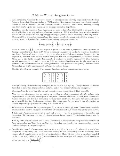
Consider the following example, if we observe 3 positive training examples as show below:
x 1 x 2 x 3 x 4 x 5 y
0 1 0 0 1 1
1 1 0 0 1 1
0 1 0 1 1 1
After processing all three training examples, we obtain h = x 2 ∧ ¯x 3 ∧ x 5 . Clearly this can be done in
time that is linear in n (the number of features) and m (the number of training examples).
This completes the proof that the concept class of boolean conjunctions is PAC learnable.
Note that one might argue that we can learn a decision tree that is consistent with the training data
in polynomial time for the second part of the proof. However, this is not a valid proof because the
learned decision tree does not necessarily (actually most likely not) belong to the hypothesis space
we are considering, i.e., boolean conjunctions. The requirement for our proof is that there exists an
efficient algorithm (poly time) for finding a consistent h ∈ C.
2. VC dimension. Consider the hypothesis space H c = circles in the (x, y) plane. Points inside the circle
are classified as positive examples. What is the VC dimension of H c ? Please fully justify your answer.
It takes only 3 parameters to specify a circle in 2-d space — the (x, y) coordinates of the center, and
the radius. We can guess that the VC dimension is no larger than 3. The following 3 points can be
shattered.
With 4 points, you can’t get all sets of size 2. Specifically, if we identify the two points that are furthest
from one another, and label them positive, and the other two negative, we cannot possibly create a
circle enclosing only the positive pairs.
3. Consider the class C of concepts of the form (a ≤ x ≤ b) ∧ (c ≤ y ≤ d), where a, b, c, and d are
integers in the interval [0, 99]. Note that each concept in this class corresponds to a rectangle with
integer-valued boundaries on a portion of the (x, y) plane. Hint: Given a region in the plane bounded
by the points (0, 0) and (n − 1, n − 1), the number of distinct rectangles with integer-valued boundaries
( ) 2 n(n − 1)
within this region is
.
2
1

Sets of size 0, 1, 3
Sets of size 2
(a) Give an upper bound on the number of randomly drawn training examples sufficient to assure
that for any target concept c in C, any consistent learner using H = C will, with probability 95%,
output a hypothesis with error at most 0.15.
We will compute the size of this hypothesis space and then apply the bound
m ≤ 1 [
ln |H| + log 1 ]
ɛ
δ
For a ≤ x ≤ b and x ∈ {0, 1, . . . , 99}, there are 100·99
2
= 4950 legal combinations. The same
argument holds for c ≤ y ≤ d. So the total number of axis-parallel rectangles is 24,502,500. The
problem specifies ɛ = 0.15 and δ = 0.05, so plugging in, we get (in lisp notation):
(* (/ 1.0 0.15) (+ (log 24502550) (log (/ 1.0 0.05)))) =
(* 6.666666666666667 (+ 17.01428775173149 2.995732273553991)) =
133.4001335019032
So we need at least 134 examples.
(b) Now suppose the rectangle boundaries a, b, c, and d take on real values instead of integer values.
Update your answer to the first part of this question.
We will compute the VC dimension of the space and apply the bound
m ≤ 1 [4 lg(2/δ) + 8d lg(13/ɛ)]
ɛ
From the previous problem, the VC dimension is 4. So this becomes
(* (/ 1.0 0.15)
(+ (* 4 (log (/ 2.0 0.05) 2))
(* 8 4 (log (/ 13.0 0.15) 2.0)))) =
(* 6.666666667
(+ 21.28771237954945 205.99696999383357)) =
1515.2312
So we need 1,516 examples.
Tom Mitchell’s ML textbook gives a nice analysis of the following algorithm. Let h be the smallest
axis-parallel rectangle that covers all of the positive training examples. If there is no noise in the
training data, then we know that h ⊆ t, where t is the true axis parallel rectangle. We can then
bound the error between h and t by the probability that a new data point will fall outside of h
but inside t. The resulting bound is
m ≥ (4/ɛ) log(4/δ).
2

The question said you should bound the error rate of a learning algorithm that chooses any
consistent rectangle. But if we restrict the algorithm to choosing the smallest consistent rectangle,
then we get a bound of 117 examples!
4. In the discussion of learning theory, a key assumption is that the training data has the same distribution
as the test data. In some cases, we might have noisy training data. In particular, we consider the binary
classification problem with labels y ∈ {0, 1}, and let D be a distribution over {x, y} that we think of
as the original uncorrupted distribution. However, we don’t directly observe from this distribution for
training. Instead, we observe from D τ , a corrupted distribution over {x, y}, which is the same as D,
except that the label y has some probability 0 < τ < 0.5 to be flipped. In other words, our training
data is generated by first sampling from D, then with probability τ (independent of the observed x
and y) replace y with 1 − y. Note that D 0 = D.
The distribution D τ models the setting in which an unreliable labeler is labeling the training data for
you, and each example has a probability τ of being mislabeled. Even though the training data is corrupted,
we are still interested in evaluating our hypotheses w.r.t. the original uncorrupted distribution
D.
We define the generalization error with respect to D τ to be:
ɛ τ = P (x,y)∼Dτ [h(x) ≠ y]
Note that ɛ 0 is the generalization error with respect to the clean distribution. It is with respect to ɛ 0
that we wish to evaluate our hypothesis.
a. For any hypothesis h, the quantity ɛ 0 (h) can be calculated as a function of ɛ τ (h) and τ. Write
down a formula for ɛ 0 (h) in terms of ɛ τ (h) and τ.
If h is correct on an instance from D 0 , it will be correct for for D τ with probability 1 − τ, and
be incorrect with probability τ. If h is incorrect on an instance from D 0 , with probability τ it
remain incorrect for D τ , and correct with probability 1 − τ. Thus we have:
Solving ɛ 0 , we have:
ɛ τ = (1 − ɛ 0 ) ∗ τ + ɛ 0 ∗ (1 − τ)
ɛ 0 = ɛ τ − τ
1 − 2τ
b. Let H be finite and suppose our training set S = {(x i , y i ) : i = 1, ..., m} is obtained by sampling
IID from D τ . Suppose we pick the hypothesis h ∈ H that minimizes the training error: ĥ =
arg min h∈H ˆɛ τ (h). Also, let h ∗ = arg min h∈H ɛ 0 (h), i.e., the optimal hypothesis in H. Let any
δ, γ > 0 be given, prove that for
ɛ 0 (ĥ) ≤ ɛ 0(h ∗ ) + 2γ
to hold with probability 1 − δ, we need to have training data size
m ≥
1 2|H|
2(1 − 2τ) 2 log
γ2 δ
Hint: you will need to use the following fact derived from Hoeffding bound:
∀h ∈ H, |ɛ τ (h) − ˆɛ τ (h)| ≤ ˆγ with probability (1 − δ), δ = 2|H| exp(−2ˆγ 2 m)
where ˆɛ τ (h) is the training error of h on training data S generated from corrupted distribution
D τ . You will also need to use the answer to subproblem (a).
we begin by note that
∀h ∈ H, |ɛ τ (h) − ˆɛ τ (h)| ≤ ˆγ with probability (1 − δ), δ = 2|H| exp(−2ˆγ 2 m)
3

Using results from the last subproblem, we have:
ɛ 0 (ĥ) = ɛ τ (ĥ) − τ ⇒
1 − 2τ
ɛ 0 (ĥ) ≤ ˆɛ τ (ĥ) − τ + ˆγ
with (1 − δ) probability ⇒
1 − 2τ
ɛ 0 (ĥ) ≤ ˆɛ τ (h ∗ ) − τ + ˆγ
with (1 − δ) probability ⇒
1 − 2τ
ɛ 0 (ĥ) ≤ ɛ τ (h ∗ ) − τ + 2ˆγ
with (1 − δ) probability ⇒
1 − 2τ
Plug in ɛ τ (h ∗ ) = (1 − 2τ)ɛ 0 (h ∗ ) + τ, we have:
ɛ 0 (ĥ) ≤ (1 − 2τ)ɛ 0(h ∗ ) + 2ˆγ
with (1 − δ) probability ⇒
1 − 2τ
ɛ 0 (ĥ) ≤ ɛ 0(h ∗ ) +
2ˆγ with (1 − δ) probability ⇒
1 − 2τ
Now do a variable exchange: γ =
γ
1−2τ
, we have:
ɛ 0 (ĥ) ≤ ɛ 0(h ∗ ) + 2γ with (1 − δ) probability, where δ = 2|H| exp(−2(γ(1 − 2τ)) 2 m
Let 2|H| exp(−2(γ(1 − 2τ)) 2 m ≤ δ, we have:
m ≥
1 2|H|
2(1 − 2τ) 2 log
γ2 δ
Remark: This suggests that m training examples that are corrupted by the noise will be worth
about (1 − 2τ) 2 m uncorrupted training examples. This is a useful rule of thumb to know if you
want to decide how much to pay for a more reliable source of training data. Also note that when
τ approaches 0.5, the labels become more and more random and the training examples eventually
becomes useless as we will need infinite amount of data in order to have any guarantee.
5. Boosting. Please show that in each iteration of Adaboost, the weighted error of h i on the updated
weights D i+1 is exactly 50%. In other words, ∑ N
j=1 D i+1(j)I(h i (X j ) ≠ y j ) = 50%.
Solution: Let ɛ i be the weighted error of h i , that is ɛ i = ∑ N
j=1 D i(j)I(h i (X j ) ≠ y j ), where I(·) is
the indicator function that takes value 1 if the argument is true, and value 0 otherwise. Following the
update rule of Adaboost, let’s assume that the weights of the correct examples are multiplied by e −γ ,
and those of the incorrect examples are multiplied by e γ . After the updates, to make sure that h i has
exactly 50% accuracy, we only need to satisfy the following:
which is exactly the value Adaboost uses.
ɛe −γ = (1 − ɛ)e γ ⇒
ɛ
1 − ɛ = e2γ ⇒
ɛ
log
1 − ɛ = 2γ ⇒
γ = 1 2 log
ɛ
1 − ɛ
4