Worksheet 42: Dijkstra's Algorithm - Classes

Worksheet 42: Dijkstra’s Algorithm
Name:
Worksheet 42: Dijkstra’s Algorithm
In worksheet 41 you investigated an algorithm to solve the problem of graph
reachablility. The exact same algorithm would perform two different types of search,
either depth-first or breadth-first search, depending upon whether a stack or a queue was
used to hold intermediate location. When dealing with weighted and directed graphs,
there is a third possibility. A common question in such graphs is not whether a given
vertex is reachable, but what is the lowest cost (that is, sum of arc weights) to reach the
vertex. This problem can be solved by using the same algorithm, storing intermediate
values in a priority queue, where the priority is given by the cost to reach the vertex. This
is known as Dijkstra’s algorithm (in honor of the computer scientist who first discovered
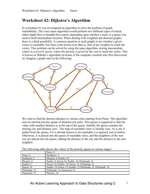
it). Imagine a graph such as the following:
We want to find the shortest distance to various cities starting from Pierre. The algorithm
uses an internal priority queue of distance/city pairs. This queue is organized so that the
value with smallest distance is at the top of the queue. Initially the queue contains the
starting city and distance zero. The map of reachable cities is initially zero. As a city if
pulled from the queue, if it is already known to be reachable it is ignored, just as before.
Otherwise, it is placed into the queue of reachable cities, and the neighbors of the new
city are placed into the queue, adding the distance to the city and the distance to the new
neighbor.
The following table shows the values of the priority queue at various stages:
Pierre: 0
Pierre: 0 Pendleton: 2
Pendleton: 2 Phoenix: 6, Pueblo: 10
Phoenix: 6 Pueblo: 9, Peoria 10, Pueblo: 10, Pittsburgh: 16
Pueblo: 9 Peoria: 10, Pueblo: 10, Pierre: 12, Pittsburgh: 16
Peoria: 10 Pueblo: 10, Pierre: 12, Pueblo: 13 Pittsburgh: 15, Pittsburgh: 16
Pittsburgh: 15 Pittsburgh: 16, Pensacola: 19
Pensacola: 19 Phoenix: 24
An Active Learning Approach to Data Structures using C 1

Worksheet 42: Dijkstra’s Algorithm
Name:
Notice how duplicates are removed only when pulled from the queue.
Simulate Dijkstra’s algorithm, only this time using Pensacola as the starting city:
An Active Learning Approach to Data Structures using C 2