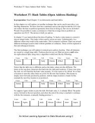
The Nearest Neighbor Algorithm - Classes

The Nearest Neighbor Algorithm
• A lazy learning algorithm
– The “learning” does not occur until the test
example is given
– In contrast to so called “eager learning”
algorithms (which carries out learning without
knowing the test example, and after learning
training examples can be discarded)

Nearest Neighbor Algorithm
• Remember all training examples
• Given a new example x, find the its closest training
example and predict y i New example
• How to measure distance – Euclidean (squared):
x − x
i
2
= ∑(
x − x
j
j
i
j
)
2

Decision Boundaries: The Voronoi Diagram
• Given a set of points,
a Voronoi diagram
describes the areas
that are nearest to
any given point.
• These areas can be
viewed as zones of
control.

Decision Boundaries: The Voronoi Diagram
• Decision boundaries are formed
by a subset of the Voronoi
diagram of the training data
• Each line segment is
equidistant between two points
of opposite class.
• The more examples that are
p
stored, the more fragmented
and complex the decision
boundaries can become.

Decision Boundaries
With large number of examples
and possible noise in the labels,
the decision i boundary can
become nasty!
We end up overfitting the data

Example:
K-Nearest Neighbor
K = 4
New example
Find the k nearest neighbors and have them vote. Has a
g
smoothing effect. This is especially good when there is noise
in the class labels.

Effect of K
K=1 K=15
Figures from Hastie, Tibshirani and Friedman (Elements of Statistical Learning)
Larger k produces smoother boundary effect and can reduce the
impact of class label noise.
But when K = N, we always predict the majority class

Question: how to choose k?
• Can we choose k to minimize the mistakes that we make
on training examples (training error)?
K=20 K=1
A model selection
problem that we will
Model complexity
study later

Distance Weighted Nearest Neighbor
• It makes sense to weight the contribution of
each example according to the distance to the
new query example
– Weight varies inversely with the distance, such that
examples closer to the query points get higher weight
• Instead of only k examples, we could allow all
training examples to contribute
– Shepard’s method (Shepard 1968)

Curse of Dimensionality
• kNN breaks down in high-dimensional space
– “Neighborhood” becomes very large.
• Assume 5000 points uniformly distributed in the unit hypercube and
we want to apply 5-nn. Suppose our query point is at the origin.
– In 1-dimension, we must go a distance of 5/5000 = 0.001 on the
average to capture 5 nearest neighbors
– In 2 dimensions, we must go 0.001 to get a square that contains
0.001 of the volume.
– In d dimensions, we must go (0.001) 1/d

The Curse of Dimensionality:
Illustration
• With 5000 points in 10 dimensions, we must go 0.501
distance along each dimension in order to find the 5
nearest neighbors

The Curse of Noisy/Irrelevant Features
• NN also breaks down when data contains irrelevant/noisy features.
• Consider a 1-d problem where query x is at the origin, our nearest
neighbor is x 1 at 0.1, and our second nearest neighbor is x 2 at 0.5.
• Now add a uniformly random noisy feature.
– P(||x 2 ’ - x||

Curse of Noise (2)
Location of x 1 versus x 2
’ - x||

Problems of k-NN
• Nearest neighbor is easily misled by noisy/irrelevant
features
• One approach: Learn a distance metric:
– that weights each feature by its ability to minimize the prediction
error, e.g., its mutual information i with the class.
– that weights each feature differently or only use a subset of
features and use cross validation to select the weights or feature
subsets
– Learning distance function is an active research area

Nearest Neighbor Summary
• Advantages
– Learning is extremely simple and intuitive,
iti – Very flexible decision boundaries
– Variable-sized hypothesis space
• Disadvantages
– distance function must be carefully chosen or tuned
– irrelevant or correlated features have high impact and must be
eliminated
– typically cannot handle high dimensionality
– computational costs: memory and classification-time time
computation
• To reduce the cost of finding nearest neighbors, use data structure
such as kd-tree