Marine Ecology Progress Series 353:289

292
Mar Ecol Prog Ser 353: 289–301, 2008
surface temperature (SST), sea surface height anomalies
(SSHA) and chlorophyll (chl) a concentration.
SST was derived from multi-channel data sensed
through the Advanced Very High Resolution Radiometer
(AVHRR) on board the NOAA 14 satellite (nominally
1 km spatial resolution). Data were gridded by
optimum interpolation by the Modular Ocean Data
Assimilation System and made available by the Naval
Research Laboratory (Stennis Space Center, Mississippi,
USA; http://www7320.nrlssc.navy.mil/altimetry).
SSHA images, derived from measurements made by
Jason, TOPEX/Poseidon, Geosat Follow-on, ERS-2 and
Envisat altimetry satellites, are available from the Colorado
Center for Astrodynamic Research (University
of Colorado, Boulder, Colorado, USA; http://argo.
colorado.edu/~realtime/gsfc_global-real-time_ssh/) in
the form of 10 d averages ending at the given date.
They reveal variations in course and speed of major
currents and identify the occurrence of mesoscale
oceanographic features, like eddies or filaments, while
SST images give indications of the general course of
the Agulhas Current. The integration of these 2 information
sources is particularly valuable for portraying
rapidly changing oceanographic features, such as
passing eddies.
Finally, ocean colour images were obtained from the
Sea-viewing Wide Field-of-view Sensor (SeaWiFS)
on board the Orb-View 2 satellite (SeaWiFS Project,
http://oceancolor.gsfc.nasa.gov/). They were used to
get indications of the chl a concentration in the upper
layers of the water column and thus, their productivity.
Additionally, we considered the existing
observations of surface Lagrangian buoys
tracked with Argos in the same region as
turtles. Drifter data were obtained from
the Atlantic Oceanographic Meteorological
Laboratory (www.aoml.noaa.gov/
phod/trinanes/xbt.html). These drifters are
equipped with a drogue that acts like an
underwater sail, helping them to move
within the current flow and minimising
wind drag (Stewart 2003). In this way, they
provide reliable information on the circulation
of the upper layers of the water column
(up to 100 m), where leatherbacks
spend most of their time (Sale et al. 2006).
To compare these routes to those of the
turtles, we chose all drifters (n = 21) that
passed through the region from 25 to
30° S, 32 to 36° E in 1996 to 2003 (see
Fig. 1b). We considered the tracks of these
drifters starting when they entered this
region and onwards. To evaluate their
speed while in the Agulhas mainstream,
the track segments running along the
eastern coast of South Africa were selected (n = 14).
The possibility of placing drifters concurrently with the
departure of turtles from nesting beaches would have
been ideal. However, in a current as geographically
stable as the Agulhas Current (Gründlingh 1983), nonsimultaneous
drifters are reliable estimators for
Lagrangian motion. This is not completely true outside
of the current itself, where a wide range of circulation
characteristics are found.
GIS software (ArcView GIS 3.2) was used to plot the
routes of turtles and drifters and to superimpose the
turtle routes on the remote sensing images. To calculate
the percentage of each turtle route determined by
ocean currents (Table 1), we summed the length of the
various segments of each turtle route that were conservatively
estimated to derive from the direct influence
of current-related features (see next paragraph),
divided by the total length of the route.
RESULTS
General movement patterns
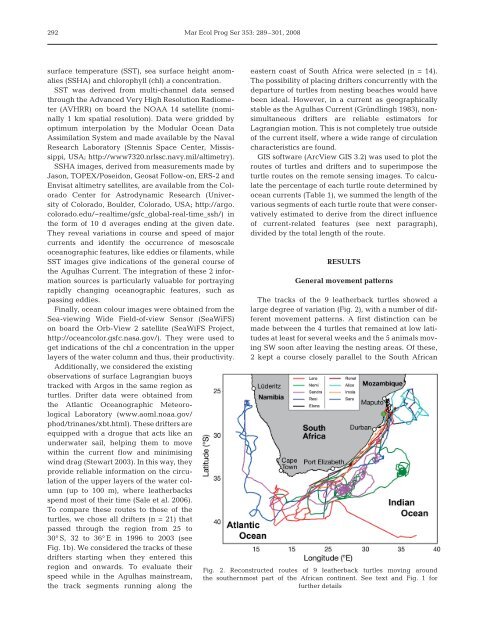
The tracks of the 9 leatherback turtles showed a
large degree of variation (Fig. 2), with a number of different
movement patterns. A first distinction can be
made between the 4 turtles that remained at low latitudes
at least for several weeks and the 5 animals moving
SW soon after leaving the nesting areas. Of these,
2 kept a course closely parallel to the South African
Fig. 2. Reconstructed routes of 9 leatherback turtles moving around
the southernmost part of the African continent. See text and Fig. 1 for
further details