algorithms

left-to-right order of Figure 6.1, we can always be sure that by the time we get to a node v,
we already have all the information we need to compute dist(v). We are therefore able to
compute all distances in a single pass:
initialize all dist(·) values to ∞
dist(s) = 0
for each v ∈ V \{s}, in linearized order:
dist(v) = min (u,v)∈E {dist(u) + l(u, v)}
Notice that this algorithm is solving a collection of subproblems, {dist(u) : u ∈ V }. We
start with the smallest of them, dist(s), since we immediately know its answer to be 0. We
then proceed with progressively “larger” subproblems—distances to vertices that are further
and further along in the linearization—where we are thinking of a subproblem as large if we
need to have solved a lot of other subproblems before we can get to it.
This is a very general technique. At each node, we compute some function of the values
of the node’s predecessors. It so happens that our particular function is a minimum of sums,
but we could just as well make it a maximum, in which case we would get longest paths in the
dag. Or we could use a product instead of a sum inside the brackets, in which case we would
end up computing the path with the smallest product of edge lengths.
Dynamic programming is a very powerful algorithmic paradigm in which a problem is
solved by identifying a collection of subproblems and tackling them one by one, smallest first,
using the answers to small problems to help figure out larger ones, until the whole lot of them
is solved. In dynamic programming we are not given a dag; the dag is implicit. Its nodes are
the subproblems we define, and its edges are the dependencies between the subproblems: if
to solve subproblem B we need the answer to subproblem A, then there is a (conceptual) edge
from A to B. In this case, A is thought of as a smaller subproblem than B—and it will always
be smaller, in an obvious sense.
But it’s time we saw an example.
6.2 Longest increasing subsequences
In the longest increasing subsequence problem, the input is a sequence of numbers a 1 , . . . , a n .
A subsequence is any subset of these numbers taken in order, of the form a i1 , a i2 , . . . , a ik where
1 ≤ i 1 < i 2 < · · · < i k ≤ n, and an increasing subsequence is one in which the numbers are
getting strictly larger. The task is to find the increasing subsequence of greatest length. For
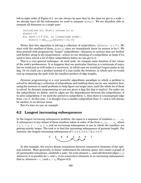
instance, the longest increasing subsequence of 5, 2, 8, 6, 3, 6, 9, 7 is 2, 3, 6, 9:
5 2 8 6 3 6 9 7
In this example, the arrows denote transitions between consecutive elements of the optimal
solution. More generally, to better understand the solution space, let’s create a graph of
all permissible transitions: establish a node i for each element a i , and add directed edges (i, j)
whenever it is possible for a i and a j to be consecutive elements in an increasing subsequence,
that is, whenever i < j and a i < a j (Figure 6.2).
162