Homework 2

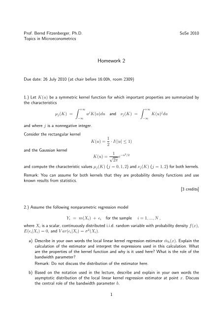
Prof. Bernd Fitzenberger, Ph.D. SoSe 2010
Topics in Microeconometrics
Homework 2
Due date: 26 July 2010 (at chair before 16:00h, room 2309)
1.) Let K(u) be a symmetric kernel function for which important properties are summarized by
the characteristics
∫ +∞
µj(K) = u j ∫ +∞
K(u)du and νj(K) = K(u) j du
−∞
and where j is a nonnegative integer.
Consider the rectangular kernel
and the Gaussian kernel
K(u) = 1
· I(|u| ≤ 1)
2
K(u) = 1
√ 2π e −u2 /2
and compute the characteristic values µj(K) (j = 0, 1, 2) and νj(K) (j = 1, 2) for both kernels.
Remark: You can assume for both kernels that they are probability density functions and use
known results from statistics.
2.) Assume the following nonparametric regression model
−∞
Yi = m(Xi) + ϵi for the sample i = 1, ..., N ,
[3 credits]
where Xi is a scalar, continuously distributed i.i.d. random variable with probability density f(x),
E(ϵi|Xi) = 0, and V ar(ϵi|Xi) = σ 2 (Xi).
a) Describe in your own words the local linear kernel regression estimator ˆmh(x). Explain the
calculation of the estimator and interpret the expressions used in this calculation. What
are the properties of the kernel function and why is it used here? What is the role of the
bandwidth parameter?
Remark: Do not discuss the distribution of the estimator here.
b) Based on the notation used in the lecture, describe and explain in your own words the
asymptotic distribution of the local linear kernel regression estimator at point x. Discuss
the central role of the bandwidth parameter h.
1

c) Simulate data using the following data generating process in TSP and implement the local
linear regression based on the Gaussian kernel. Use Silverman’s rule of thumb and crossvalidation
to determine the bandwidth parameter h. For cross validation, implement grid
search around the rule of thumb estimate. Compare the results.
TSP–Code:
options crt,mem=20,double,limwarn=0;
supres smpl;
options crt, mem=20;
smpl 1 100; set nob = @nob;
set seedin =14;
random(seedin=14) x eps;
y = 1+ x -x^2 + eps/3;
sort(all) x;
msd(noprint,all) x;
SET H00h00=@Stddev;
if @iqr/1.349

es2 = (y - @coef(1))**2;
enddo;
select 1;
msd(noprint) res2;
set sumres2 = @sum;
print h sumres2;
if (sumres2 .lt. sumres2cv); then; do;
set sumres2cv = sumres2;
set hmincv = h;
enddo;
enddo;
title ’Minimum CV’;
print hmincv sumres2cv;
llinreg y x hmincv mhat;
graph(preview) x y mhat;
proc llinreg y00 x00 h00 mhat00;
?
? Procedure for locally linear kernel regressions
?
local z00 xi00 w00 i dxi00;
supres smpl;
genr mhat00 = 0;
? supresses unnecessary calculations
regopt(nocalc) regout auto het;
do i = 1 to @nob;
set xi00 = x00(i);
genr w00 = norm((x00-xi00)/h00); ?msd(terse) w00;
genr dxi00 = x00-xi00;
? select w00 .gt. 1.d-8;
olsq(silent,weight=w00) y00 c dxi00;
set mhat00(i) = @coef(1);
? select 1;
enddo;
? reinstall default options
regopt; supres smpl;
endproc;
END;
3

Remark: The solutions to the problem 2c) should include the TSP–programs, which you
wrote to solve the problems, together with the output on paper. The discussion of the
results should make reference to the computer output.
[ 7 credits ]
3.) For a panel of length T = 2, recall that the first differences (FD) estimator for the outcome
equation
(0) yit = θt + zitγ + δ1progit + ci + uit
yields the conditional difference–in–differences (CDiD) estimator of the treatment effect δ1, when
the policy is introduced in period 2, i.e. progi1 = 0, and participation takes only place in period
2, i.e. progi2 = 0, 1. This estimator accounts for the possibility that progit is correlated with ci.
a) Motivate and describe the FD estimator above in detail. Why does it provide a consistent
estimate of the treatment effect δ1?
b) Discuss and describe a semiparametric matching estimator as an extension of the CDiD
estimator for the model
(S) yit = θt + g(zit) + δ1progit + ci + uit .
under the above setup, where the policy is introduced in period 2. Assume that zit is a
scalar regressor. Be as specific as possible.
[ 4 credits ]
4.) (Sharp RDD with simulated Data, PC Pool Problem Set 3, Problem 3)
Assume that a sample of N observations is simulated based on the following regression model
yi = 1 + α · Di + x1i − 0.1x 2 1i + x2i − 0.2x1ix2i + ϵi ,
where x1i, x2i, and ϵi are three independent random variables following a standard normal distribution.
The treatment dummy is given by
Di = I(x1i > 0.2) .
a) First assume that the treatment effect α = 3 is a fixed constant. Show that the conditions
for a sharp RDD are satisfied here, i.e. the RDD estimator identifies α. Consider the assumptions
put forward in Van der Klaauw (2002) and check formally that they are satisfied
in this case. Motivate the identification result. What is the control function k(S) in this
context? Be as specific as possible.
b) Why is it not necessary that the RDD estimator controls for x2?
4

c) Is there a discontinuous jump in the distribution of x2 at the RDD threshold ¯x1 = 0.2?
How could one implement a test for this?
d) Now assume that the treatment effect α is random with E(α) = 3 and the distribution of
α is independent of (x1, x2). Show that the conditions for a sharp RDD are satisfied here
as well, i.e. the RDD estimator identifies α. Consider the assumptions put forward in Van
der Klaauw (2002) and check formally that they are satisfied in this case. Motivate the
identification result. What is the control function k(S) in this context? Be as specific as
possible.
Remark: This is a theoretical exercise. To solve this problem, it is not necessary to implement a
TSP program for estimation purposes.
[ 7 credits ]
5.) (Fuzzy RDD: Angrist and Lavy 1999, Maimonides Rule, PC Pool Problem Set 3, Problem 4)
Use the programs and the data provided as part of the third PC Pool Problem Set. For the
problem analyze only math scores as outcome variables for the fourth grade.
a) Analyze whether the variable ’percent disadvantaged’ shows discontinuous jumps at the
tresholds used to split classes. What do these results imply regarding the question as to
whether it is necessary to control for the variable ’percent disadvantaged’ when estimating
the RDD estimate of the treatment effect of class size?
b) Implement the 2SLS estimate of the effect of class size on math scores in the fourth grade
controlling for enrollment using an appropriate polynomial specification of enrollemnt and
percent disadvantaged as control variables. Discuss the results.
c) Implement the local Wald estimator for the RDD based on a local linear regression (using
a rectangular kernel) of class size on expected class size on both sides of each threshold.
Use these nonparametric estimates from the first stage to estimate in a second stage the
fuzzy RDD estimate of the effect of class size
E(Yi|
ˆρs = lim
∆→0
¯ Ss < S < ¯ Ss + ∆) − E(Yi| ¯ Ss − ∆ < S < ¯ Ss)
E(Di| ¯ Ss < S < ¯ Ss + ∆) − E(Di| ¯ Ss − ∆ < S < ¯ Ss)
for the s th threshold ¯ Ss (using the notation in the lecture). Discuss the differences in
methods and results in comparison to part b).
Remark: The solutions to the problem should include the TSP–programs, which you wrote to
solve the problems, together with the output on paper. The discussion of the results should make
reference to the computer output.
5
[ 6 credits ]