The Effect of Temperature on Microstructure of Lead-free Solder Joints
The Effect of Temperature on Microstructure of Lead-free Solder Joints
The Effect of Temperature on Microstructure of Lead-free Solder Joints

Create successful ePaper yourself
Turn your PDF publications into a flip-book with our unique Google optimized e-Paper software.
NPL Report MATC(A)157<br />
<str<strong>on</strong>g>The</str<strong>on</strong>g> <str<strong>on</strong>g>Effect</str<strong>on</strong>g> <str<strong>on</strong>g>of</str<strong>on</strong>g> <str<strong>on</strong>g>Temperature</str<strong>on</strong>g> <strong>on</strong> <strong>Microstructure</strong> <str<strong>on</strong>g>of</str<strong>on</strong>g><br />
<strong>Lead</strong>-<strong>free</strong> <strong>Solder</strong> <strong>Joints</strong><br />
Thomas Le Toux, Milos Dusek & Christopher Hunt<br />
November 2003
<str<strong>on</strong>g>The</str<strong>on</strong>g> <str<strong>on</strong>g>Effect</str<strong>on</strong>g> <str<strong>on</strong>g>of</str<strong>on</strong>g> <str<strong>on</strong>g>Temperature</str<strong>on</strong>g> <strong>on</strong> <strong>Microstructure</strong><br />
<str<strong>on</strong>g>of</str<strong>on</strong>g><br />
<strong>Lead</strong>-<strong>free</strong> <strong>Solder</strong> <strong>Joints</strong><br />
Thomas Le Toux, Milos Dusek and Christopher Hunt<br />
Nati<strong>on</strong>al Physical Laboratory<br />
Teddingt<strong>on</strong>, Middlesex, UK, TW11 0LW<br />
ABSTRACT<br />
Samples <str<strong>on</strong>g>of</str<strong>on</strong>g> surface mounted comp<strong>on</strong>ents cooled during their solidificati<strong>on</strong> process were<br />
subjected to aging treatment in accelerated way to develop microstructural changes.<br />
Microsecti<strong>on</strong>s <str<strong>on</strong>g>of</str<strong>on</strong>g> solder joints were analysed and methods for measurement <str<strong>on</strong>g>of</str<strong>on</strong>g> characteristic<br />
size <str<strong>on</strong>g>of</str<strong>on</strong>g> Sn-dendrite is proposed. <str<strong>on</strong>g>The</str<strong>on</strong>g>se tools can be used to detect structures (such as<br />
dendrites, dendrites grains, or intermetallic features).<br />
<str<strong>on</strong>g>The</str<strong>on</strong>g> impact <str<strong>on</strong>g>of</str<strong>on</strong>g> cooling rate and iso-thermal ageing <strong>on</strong> the microstructure <str<strong>on</strong>g>of</str<strong>on</strong>g> lead-<strong>free</strong> alloys as<br />
used in surface mount joints is investigated. <str<strong>on</strong>g>The</str<strong>on</strong>g> changes in the tin dendrites and<br />
intermetallics are measured using image analysis tools developed here. <str<strong>on</strong>g>The</str<strong>on</strong>g> algorithm<br />
developed produces a numerated classificati<strong>on</strong> that can be correlated with the aging <str<strong>on</strong>g>of</str<strong>on</strong>g> the<br />
microstructure.
© Crown copyright 2003<br />
Reproduced by permissi<strong>on</strong> <str<strong>on</strong>g>of</str<strong>on</strong>g> the C<strong>on</strong>troller <str<strong>on</strong>g>of</str<strong>on</strong>g> HMSO<br />
ISSN 1473 2734<br />
Nati<strong>on</strong>al Physical Laboratory<br />
Teddingt<strong>on</strong>, Middlesex, UK, TW11 0LW<br />
Extracts from this report may be reproduced provided the source is<br />
acknowledged.<br />
Approved <strong>on</strong> behalf <str<strong>on</strong>g>of</str<strong>on</strong>g> Managing Director, NPL, by Dr C Lea,<br />
Head, Materials Centre
C<strong>on</strong>tents<br />
1.1. INTRODUCTION....................................................................................................2<br />
1.2. DESCRIPTION OF TEST SPECIMENS ....................................................................2<br />
1.2.1. Examinati<strong>on</strong> <str<strong>on</strong>g>of</str<strong>on</strong>g> dendrites ............................................................................... 4<br />
1.2.2. Intermetallic layer al<strong>on</strong>g interfaces ................................................................ 6<br />
1.3. INTERMETALLIC FLAKES..........................................................................................8<br />
1.4. DETECTING FINE AND COARSE STRUCTURES OF DENDRITES...................................10<br />
1.4.1. Detecting dendrite directi<strong>on</strong>..........................................................................14<br />
2. CONCLUSIONS ........................................................................................................23<br />
3. REFERENCES...........................................................................................................24<br />
4. ACKNOWLEDGEMENTS .......................................................................................24
NPL Report MATC(A)157<br />
1.1. Introducti<strong>on</strong><br />
Mechanical testing <str<strong>on</strong>g>of</str<strong>on</strong>g> lead-<strong>free</strong> solders has been under extensive research over last 5 years.<br />
<str<strong>on</strong>g>The</str<strong>on</strong>g> industry currently has the benefit if more than 40 years <str<strong>on</strong>g>of</str<strong>on</strong>g> reliability data with standard<br />
SnPb alloy. As the industry moves forward there is an urgent need to acquire the equivalent<br />
data for the lead-<strong>free</strong> alloy <str<strong>on</strong>g>of</str<strong>on</strong>g> choice over a compressed time scale. Major reas<strong>on</strong>s for<br />
c<strong>on</strong>cerns in using lead-<strong>free</strong> solders are lack <str<strong>on</strong>g>of</str<strong>on</strong>g> reliability and processability for lead-<strong>free</strong><br />
alloys. Alloy reliability will be very much a functi<strong>on</strong> <str<strong>on</strong>g>of</str<strong>on</strong>g> the microstructure, which in turns<br />
affects properties such as strength, creep, stress relaxati<strong>on</strong> and so <strong>on</strong>. Clearly <strong>on</strong>ly<br />
relati<strong>on</strong>ship that can be established between microstructure and mechanical properties would<br />
be very valuable. However characterising microstructure is complex, a significant issue being<br />
the analysis is run <strong>on</strong> a 2D image, where in actuality the analysis is <str<strong>on</strong>g>of</str<strong>on</strong>g> the 3D structure. <str<strong>on</strong>g>The</str<strong>on</strong>g><br />
approach here is to use features occurring in the microsecti<strong>on</strong>s, measure these and attempt to<br />
correlate these with mechanical properties. Further more in this report the effect <str<strong>on</strong>g>of</str<strong>on</strong>g> cooling<br />
rate and temperature c<strong>on</strong>diti<strong>on</strong>ing <strong>on</strong> the microstructure <str<strong>on</strong>g>of</str<strong>on</strong>g> lead-<strong>free</strong> solder joints has been<br />
investigated.<br />
Tin-silver based solder alloys are leading candidates for lead-<strong>free</strong> solders in electr<strong>on</strong>ic<br />
manufacturing. <str<strong>on</strong>g>The</str<strong>on</strong>g> mechanical performance <str<strong>on</strong>g>of</str<strong>on</strong>g> a surface mount solder joint depends <strong>on</strong> its<br />
microstructure and this has to be assessed, as a functi<strong>on</strong> <str<strong>on</strong>g>of</str<strong>on</strong>g> processing and storage c<strong>on</strong>diti<strong>on</strong>s.<br />
<strong>Microstructure</strong> can be captured by taking cross-secti<strong>on</strong>al images <str<strong>on</strong>g>of</str<strong>on</strong>g> solder joints, and then<br />
processed by image analysers to obtain summarised informati<strong>on</strong> about the complex<br />
microstructure.<br />
1.2. Descripti<strong>on</strong> <str<strong>on</strong>g>of</str<strong>on</strong>g> test specimens<br />
Table 1 lists <str<strong>on</strong>g>of</str<strong>on</strong>g> sample <str<strong>on</strong>g>of</str<strong>on</strong>g> aging c<strong>on</strong>diti<strong>on</strong>s and includes various aging temperatures and times<br />
al<strong>on</strong>g with various cooling rates from the molten solder state. <str<strong>on</strong>g>The</str<strong>on</strong>g> examples <str<strong>on</strong>g>of</str<strong>on</strong>g><br />
microsectioend specimens are shown in Figure 1 for BGA, SOIC and chip resistor joints.<br />
<str<strong>on</strong>g>The</str<strong>on</strong>g>re are two lead-<strong>free</strong> solders used in the experiment Sn3.5Ag and Sn3.5Ag0.7Cu.<br />
BGA SOIC 0805 chip resistor<br />
Figure 1: Examples <str<strong>on</strong>g>of</str<strong>on</strong>g> optical micrographs<br />
2
NPL Report MATC(A)157<br />
Table 1 <str<strong>on</strong>g>The</str<strong>on</strong>g>rmal c<strong>on</strong>diti<strong>on</strong>s <str<strong>on</strong>g>of</str<strong>on</strong>g> the specimens<br />
Aging Cooling<br />
Designati<strong>on</strong> Alloy <str<strong>on</strong>g>Temperature</str<strong>on</strong>g> Time rate<br />
[°C] [hours] [°C/s]<br />
m429 SnAgCu 20 0 0.5<br />
m450 SnAg 20 0 0.5<br />
m428 SnAgCu 20 0 1<br />
m449 SnAg 20 0 1<br />
m427 SnAgCu 20 0 2<br />
m448 SnAg 20 0 2<br />
m426 SnAgCu 20 400 0.5<br />
m425 SnAgCu 20 400 1<br />
m424 SnAgCu 20 400 2<br />
m414 SnAgCu 50 400 0.5<br />
m413 SnAgCu 50 400 0.5<br />
m439 SnAg 50 400 2<br />
m420 SnAgCu 125 400 0.5<br />
m415 SnAgCu 125 400 2<br />
m416 SnAgCu 125 400 2<br />
m412 SnAgCu 50 1000 0.5<br />
m47 SnAgCu 50 1000 2<br />
m45 SnAgCu 125 1000 0.5<br />
m46 SnAgCu 125 1000 0.5<br />
m44 SnAgCu 125 1000 1<br />
m431 SnAg 125 1000 1<br />
Analysis <str<strong>on</strong>g>of</str<strong>on</strong>g> micrographs involves, identificati<strong>on</strong> <str<strong>on</strong>g>of</str<strong>on</strong>g> comm<strong>on</strong> structures such as intermetallics<br />
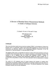
and tin dendrites. <str<strong>on</strong>g>The</str<strong>on</strong>g> typical microstructure <str<strong>on</strong>g>of</str<strong>on</strong>g> samples is identified in Figure 2.<br />
h<br />
g<br />
f<br />
d<br />
e<br />
c<br />
b<br />
a<br />
Figure 2: M449BGA7 tin-silver sample<br />
3
NPL Report MATC(A)157<br />
a PCB interc<strong>on</strong>necti<strong>on</strong>. This is a copper layer pad with thickness <str<strong>on</strong>g>of</str<strong>on</strong>g> 35 µm<br />
b 0.5 µm thin Nickel layer<br />
c Cu 6 Sn 5 and Cu 3 Sn intermetallic layer with Ni, forming thin “needles” (not clear at this scale)<br />
dAg 3 Sn “flake”<br />
e Ag 3 Sn structure oriented perpendicular to structure (d) in lateral plane<br />
f tin dendrites (white)<br />
g matrix <str<strong>on</strong>g>of</str<strong>on</strong>g> Sn, with Ag 3 Sn lamellae (black)<br />
h comp<strong>on</strong>ent interc<strong>on</strong>necti<strong>on</strong>: Cu layer with a Ni barrier (solder mask defined)<br />
As seen in Figure 2 the flake (e) is oriented parallel to microstructural plain which in fact is<br />
the same structure as (d).<br />
1.2.1. Examinati<strong>on</strong> <str<strong>on</strong>g>of</str<strong>on</strong>g> dendrites<br />
Sn dendrites are the main visual structures, which can be identified in micrographs from<br />
either optical <str<strong>on</strong>g>of</str<strong>on</strong>g> SEM images. We can observe <strong>on</strong> micrographs that dendrites are <str<strong>on</strong>g>of</str<strong>on</strong>g>ten<br />
gathered within col<strong>on</strong>ies shown schematically in Figure 3. <str<strong>on</strong>g>The</str<strong>on</strong>g> dendrite stems within any <strong>on</strong>e<br />
col<strong>on</strong>y are all crystallo-graphically related to a comm<strong>on</strong> nucleus.<br />
Figure 3: Dendrites grains. <str<strong>on</strong>g>The</str<strong>on</strong>g> mould wall relates to comp<strong>on</strong>ents interc<strong>on</strong>necti<strong>on</strong>s<br />
Figure 4 illustrates typical tin dendrite formati<strong>on</strong>; the figure also reveals a trapped void inside<br />
the joint, caused by entrapped gases solidified in the solder joint.<br />
4
NPL Report MATC(A)157<br />
Figure 4: dendrites <strong>on</strong> M429BGA5<br />
Since a dendrite is a three-dimensi<strong>on</strong>al object its appearance <strong>on</strong> a 2D photograph depends<br />
up<strong>on</strong> the plane <str<strong>on</strong>g>of</str<strong>on</strong>g> the secti<strong>on</strong>.<br />
Figure 5: col<strong>on</strong>ies <str<strong>on</strong>g>of</str<strong>on</strong>g> dendrites, M429BGA5<br />
Analyses have been performed <strong>on</strong> several samples with a Scanning Electr<strong>on</strong> Microscope<br />
(SEM), to c<strong>on</strong>firm the elemental c<strong>on</strong>stituti<strong>on</strong> <str<strong>on</strong>g>of</str<strong>on</strong>g> each structure in the micrographs. While the<br />
data is c<strong>on</strong>sistent with the expected result the analysed depth, typically few µm may lead to<br />
some small errors, and is not thought to be an issue in the following work.<br />
5
NPL Report MATC(A)157<br />
1.2.2. Intermetallic layer al<strong>on</strong>g interfaces<br />
<str<strong>on</strong>g>The</str<strong>on</strong>g>se joints show a typical intermetallic layer forming at the interface. <str<strong>on</strong>g>The</str<strong>on</strong>g> intermetallic<br />
layer thickness increases with time and temperature [1]. <str<strong>on</strong>g>The</str<strong>on</strong>g> starting point <str<strong>on</strong>g>of</str<strong>on</strong>g> the analysis is<br />
to crop images from the various specimens to be evaluated, and c<strong>on</strong>verting the images into a<br />
256 grey scale format. Images in this format have better clarity, and are less sensitive to<br />
brightness & c<strong>on</strong>trast settings when using colour images. <str<strong>on</strong>g>The</str<strong>on</strong>g> resulting image is shown in<br />
Figure 7a. <str<strong>on</strong>g>The</str<strong>on</strong>g> transform into a binary image was based <strong>on</strong> a grey-level histogram (Figure 7b)<br />
<str<strong>on</strong>g>of</str<strong>on</strong>g> the image.<br />
a)<br />
b)<br />
Figure 6:<str<strong>on</strong>g>The</str<strong>on</strong>g> grey image, the greyscale and the histogram (<strong>on</strong> the horiz<strong>on</strong>tal axis are the<br />
grey levels, and <strong>on</strong> the vertical <strong>on</strong>e are the numbers <str<strong>on</strong>g>of</str<strong>on</strong>g> pixels in the image for each grey<br />
level). Grey levels are coded between 0 and 1, at 256 discrete values.<br />
<str<strong>on</strong>g>The</str<strong>on</strong>g> histogram (Figure 8) was analysed for peaks and a threshold limit was set <strong>on</strong> the local<br />
minimum (dip) in between light and dark peak. For example at the local minimum located at<br />
about 0.65 (<str<strong>on</strong>g>of</str<strong>on</strong>g> greyscale), all pixels left <str<strong>on</strong>g>of</str<strong>on</strong>g> the threshold are turned into black and pixels <strong>on</strong><br />
the right were made white.<br />
Figure 7: <str<strong>on</strong>g>The</str<strong>on</strong>g> histogram and the threshold; the red curve is smoothed by cubic splines, in<br />
order to detect the local minimum<br />
6
NPL Report MATC(A)157<br />
<str<strong>on</strong>g>The</str<strong>on</strong>g> resulting binary image is shown in Figure 9. As not all images will generate the same<br />
histograms (with a local minimum at 0.65), an automatic threshold method was used. Other<br />
commercially available methods can be used such as the Otsu’s method [].<br />
Ag 3 Sn plates<br />
White Sn dendrites<br />
Cu 6 Sn 5<br />
intermetallics<br />
Figure 8: the resulting binary image<br />
Identificati<strong>on</strong> <str<strong>on</strong>g>of</str<strong>on</strong>g> the white and black areas <strong>on</strong> this binary image; in our sample (M449BGA7<br />
Figures 9) are as follows:<br />
• Black = Lamellae Ag 3 Sn in the Sn matrix and the intermetallic layer al<strong>on</strong>g<br />
interface<br />
• White = Sn dendrites and Ag 3 Sn plates<br />
C<strong>on</strong>cerning the intermetallic interface, this appears as a solid black area (at the bottom <str<strong>on</strong>g>of</str<strong>on</strong>g><br />
Figure 9). To extract this feature, and measure its thickness, a process for detecting areas <str<strong>on</strong>g>of</str<strong>on</strong>g> a<br />
comm<strong>on</strong> type was used (segmentati<strong>on</strong>).<br />
Figure 9 Segmentati<strong>on</strong> <str<strong>on</strong>g>of</str<strong>on</strong>g> an image into comp<strong>on</strong>ents<br />
In the segmentati<strong>on</strong> procedure a specific area is selected and coloured by the simple rule that<br />
adjacent pixels to each other by at least <strong>on</strong>e side <str<strong>on</strong>g>of</str<strong>on</strong>g> the pixel from either black or white<br />
7
NPL Report MATC(A)157<br />
regi<strong>on</strong>s. <str<strong>on</strong>g>The</str<strong>on</strong>g>se c<strong>on</strong>nected areas are called “comp<strong>on</strong>ents” and are indexed with a single<br />
number. In our example we have identified 63 comp<strong>on</strong>ents in the image Figure 10.<br />
<str<strong>on</strong>g>The</str<strong>on</strong>g> intermetallic layer is manually selected, and here is represented by c<strong>on</strong>tinuous regi<strong>on</strong> at<br />
the bottom <str<strong>on</strong>g>of</str<strong>on</strong>g> the image. <str<strong>on</strong>g>The</str<strong>on</strong>g> average height <str<strong>on</strong>g>of</str<strong>on</strong>g> intermetallic was calculated by counting the<br />
number <str<strong>on</strong>g>of</str<strong>on</strong>g> pixels in this comp<strong>on</strong>ent and divided by the image width in pixels. A<br />
computati<strong>on</strong>al approach was largely unsuccessful due to problems in distinguishing between<br />
natural tin dendrite structures and that <str<strong>on</strong>g>of</str<strong>on</strong>g> the intermetallics.<br />
1.3. Intermetallic Flakes<br />
<str<strong>on</strong>g>The</str<strong>on</strong>g> intermetallic flakes <str<strong>on</strong>g>of</str<strong>on</strong>g> Ag 3 Sn have comm<strong>on</strong> characteristic that they appear as either<br />
straight lines or flat flakes. By using the Hough transformati<strong>on</strong> straight elements in images<br />
can be detected. <str<strong>on</strong>g>The</str<strong>on</strong>g> basic idea <str<strong>on</strong>g>of</str<strong>on</strong>g> this transform is depicted in Figure 11. Assuming there is a<br />
blue straight line in the image, usually defined by its slope and its intersecti<strong>on</strong> with the y-axis.<br />
However, we can also describe this line with its perpendicular distance r 0 to the origin, and<br />
the angle θ 0 between r 0 and the x-axis. <str<strong>on</strong>g>The</str<strong>on</strong>g>refore, the original straight line is now a point in<br />
Figure 10b).<br />
a) b)<br />
c) d)<br />
Figure 10 Descripti<strong>on</strong> <str<strong>on</strong>g>of</str<strong>on</strong>g> the Hough transform<br />
A typical algorithm that uses this transform is the following: each time a white pixel is<br />
encountered <strong>on</strong> the dotted line in Figure 11c), the accumulator is incremented at the line<br />
coordinates. For instance, in Figure 10c), the blue line is made <str<strong>on</strong>g>of</str<strong>on</strong>g> four adjacent pixels with<br />
the centres marked, the value <str<strong>on</strong>g>of</str<strong>on</strong>g> the accumulator is therefore 4 at coordinates (r 0 , θ 0 ) shown in<br />
Figure 10d). Thus the l<strong>on</strong>ger the line, the higher the value in the accumulator. <str<strong>on</strong>g>The</str<strong>on</strong>g> Hough<br />
transformati<strong>on</strong> <strong>on</strong>ly works <strong>on</strong> edges or lines, so to use the transform, Figure 9 must be<br />
c<strong>on</strong>verted with an edge detecti<strong>on</strong> algorithm, as shown in Figure 12.<br />
8
NPL Report MATC(A)157<br />
Figure 11 <str<strong>on</strong>g>The</str<strong>on</strong>g> image (Figure 9) c<strong>on</strong>verted with edge detecti<strong>on</strong> algorithm<br />
Pixel<br />
count<br />
r<br />
Θ<br />
Figure 12 3 D plot <str<strong>on</strong>g>of</str<strong>on</strong>g> accumulator for figure 11<br />
Figure 12 is a 3D visual representati<strong>on</strong> <str<strong>on</strong>g>of</str<strong>on</strong>g> the accumulator matrix and shows a clear peak<br />
corresp<strong>on</strong>ding to the l<strong>on</strong>g Ag 3 Sn intermetallic.<br />
Figure 13 shows an overlay <str<strong>on</strong>g>of</str<strong>on</strong>g> the identified peak coordinate (i.e. line characterized by<br />
coordinates (r, Θ) and the original image, which shows that the algorithm is working.<br />
9
NPL Report MATC(A)157<br />
Figure 13: C<strong>on</strong>firms by plotting overlay <str<strong>on</strong>g>of</str<strong>on</strong>g> the r, Θ back <strong>on</strong>to the Figure 8 showing<br />
Having identified the flakes, when present (which is a functi<strong>on</strong> <str<strong>on</strong>g>of</str<strong>on</strong>g> the microsecti<strong>on</strong>) we now<br />
c<strong>on</strong>sider the tin dendrite structure.<br />
1.4. Detecting Fine and Coarse Structures <str<strong>on</strong>g>of</str<strong>on</strong>g> Dendrites<br />
Here we attempt to size the original white tin dendrites as can be seen <strong>on</strong> image M429BGA5<br />
(Figure 8), we can distinguish a fine structure <str<strong>on</strong>g>of</str<strong>on</strong>g> dendrites at the top <str<strong>on</strong>g>of</str<strong>on</strong>g> the picture and a<br />
coarse structure at the bottom. <str<strong>on</strong>g>The</str<strong>on</strong>g> strategy is to remove the areas where the dendrite<br />
directi<strong>on</strong> cannot be determined.<br />
<str<strong>on</strong>g>The</str<strong>on</strong>g> method is to characterize the dendrite size throughout whole image. <str<strong>on</strong>g>The</str<strong>on</strong>g> approach is to<br />
draw random lines across the image, see Figure 14 and to record the length <str<strong>on</strong>g>of</str<strong>on</strong>g> c<strong>on</strong>tinuous<br />
white or black pixels al<strong>on</strong>g the line this is plotted in Figure 15. <str<strong>on</strong>g>The</str<strong>on</strong>g>se lengths are then plotted<br />
in a histogram, in Figure 16 and peak positi<strong>on</strong> recorded. This peak, se Figure 16 is the<br />
average length <str<strong>on</strong>g>of</str<strong>on</strong>g> white-pixel peaks, i.e. the average length without crossing a black pixel this<br />
parameter characterizes the size <str<strong>on</strong>g>of</str<strong>on</strong>g> dendrites.<br />
10
NPL Report MATC(A)157<br />
Figure 14: the random path across a binary image; the intensity pr<str<strong>on</strong>g>of</str<strong>on</strong>g>ile value is<br />
represented in 3D between 0 and 1.<br />
Unsorted values <str<strong>on</strong>g>of</str<strong>on</strong>g> white lengths <strong>on</strong> path<br />
Figure 15: plot representing the length al<strong>on</strong>g the path <str<strong>on</strong>g>of</str<strong>on</strong>g> each white peak;<br />
for example, the peak #3000 about ~ 100 pixels length.<br />
11
NPL Report MATC(A)157<br />
Figure 16: Probability density functi<strong>on</strong> <str<strong>on</strong>g>of</str<strong>on</strong>g> peak sizes. 1.6 pixels peaks are more likely to<br />
occur, and the mean size <str<strong>on</strong>g>of</str<strong>on</strong>g> peaks is 10.2 pixels (1 pixels ~10µm)<br />
This approach must actually be applied <strong>on</strong> a small scale to get useful measurements, and then<br />
move this analysis area over whole image in a step-wise fashi<strong>on</strong>. <str<strong>on</strong>g>The</str<strong>on</strong>g> random pr<str<strong>on</strong>g>of</str<strong>on</strong>g>ile is run<br />
over a mask <str<strong>on</strong>g>of</str<strong>on</strong>g> 5x5 pixels and the result (the mean length) is stored at the centre pixel<br />
positi<strong>on</strong> in the output matrix, the mask is sequentially moved across the image repeating the<br />
procedure.<br />
<str<strong>on</strong>g>The</str<strong>on</strong>g>re are two opti<strong>on</strong>s in the moving the mask:<br />
1. Move by mask size, generating a course map<br />
2. Move mask by a single pixel, generating a fine map<br />
Figure 19 shows the result <str<strong>on</strong>g>of</str<strong>on</strong>g> using the fine map approach.<br />
Figure 17 top left: original binary image, top right: coarse map <str<strong>on</strong>g>of</str<strong>on</strong>g> average lengths <str<strong>on</strong>g>of</str<strong>on</strong>g> white peaks across<br />
the image (mask = 51), bottom left: fine map (mask = 51)<br />
On these two types <str<strong>on</strong>g>of</str<strong>on</strong>g> image, it is not easy to apply an efficient threshold to separate the fine<br />
and coarse structures. Another functi<strong>on</strong> has been developed, which aligns these two maps,<br />
12
NPL Report MATC(A)157<br />
using a weighted average between the values and the following was found to give the best<br />
results:<br />
• the fine pr<str<strong>on</strong>g>of</str<strong>on</strong>g>ile weights as 2<br />
• the coarse <strong>on</strong>e weights as 1<br />
<str<strong>on</strong>g>The</str<strong>on</strong>g> result is shown below (Figure 18). In Appendix II you can find other maps with different<br />
weights for the same image.<br />
Figure 18: weighted average between the coarse and fine pr<str<strong>on</strong>g>of</str<strong>on</strong>g>iles<br />
<str<strong>on</strong>g>The</str<strong>on</strong>g>n it is possible to apply a threshold to this map, in order to separate fine and coarse<br />
structures; this is a result with a threshold value <str<strong>on</strong>g>of</str<strong>on</strong>g> 5 pixels (Figure 19):<br />
Figure 19: binary map after applicati<strong>on</strong> <str<strong>on</strong>g>of</str<strong>on</strong>g> a<br />
threshold <str<strong>on</strong>g>of</str<strong>on</strong>g> 5<br />
Figure 20: the corresp<strong>on</strong>ding coarse area <strong>on</strong><br />
the original image<br />
After some tests, the value <str<strong>on</strong>g>of</str<strong>on</strong>g> 5 pixels seems to be here the optimal mask size. <str<strong>on</strong>g>The</str<strong>on</strong>g> Figure 19<br />
is multiplied by the original image to give Figure 20, and we can now clearly see large<br />
dendrites in this area. <str<strong>on</strong>g>The</str<strong>on</strong>g> next step then is to measure the dendrite orientati<strong>on</strong> and size.<br />
13
NPL Report MATC(A)157<br />
1.4.1. Detecting dendrite directi<strong>on</strong><br />
Microsecti<strong>on</strong>s <str<strong>on</strong>g>of</str<strong>on</strong>g> tin rich alloys typically form a number <str<strong>on</strong>g>of</str<strong>on</strong>g> col<strong>on</strong>ies at random orientati<strong>on</strong>s.<br />
Within any <strong>on</strong>e col<strong>on</strong>y the dendrite has a characteristic feature size for all the dendrites,<br />
where this feature maybe the length or width <str<strong>on</strong>g>of</str<strong>on</strong>g> the dendrite. <str<strong>on</strong>g>The</str<strong>on</strong>g>refore, by identifying the<br />
orientati<strong>on</strong> <str<strong>on</strong>g>of</str<strong>on</strong>g> the dendrites, the col<strong>on</strong>ies are identified and hence the dendrite measurement<br />
technique can be applied to each col<strong>on</strong>y.<br />
This method used has comm<strong>on</strong> characteristics with the previous <strong>on</strong>e, and is described trough<br />
an example in Figure 21:<br />
• white dendrites oriented north-east / south-west. <str<strong>on</strong>g>The</str<strong>on</strong>g> goal is to detect that<br />
directi<strong>on</strong>.<br />
• in blue there is a set <str<strong>on</strong>g>of</str<strong>on</strong>g> diameters in a circular shape, with a <strong>on</strong>e-degree<br />
increment.<br />
Figure 21: the new circular shape pr<str<strong>on</strong>g>of</str<strong>on</strong>g>ile to detect dendrites directi<strong>on</strong>s<br />
With each line in the circular set, the following algorithm is performed:<br />
• if the centre pixel is white, the percentage <str<strong>on</strong>g>of</str<strong>on</strong>g> white pixels <strong>on</strong> the line is<br />
returned<br />
• if the centre pixel is black, the percentage <str<strong>on</strong>g>of</str<strong>on</strong>g> black pixels is given.<br />
<str<strong>on</strong>g>The</str<strong>on</strong>g> distributi<strong>on</strong> <str<strong>on</strong>g>of</str<strong>on</strong>g> lengths (white or black pixels) for each angle is plotted in Figure 22. Later<br />
the origin <str<strong>on</strong>g>of</str<strong>on</strong>g> this circle (a sampled cell) will be moved in an incremental fashi<strong>on</strong> throughout<br />
the image.<br />
14
NPL Report MATC(A)157<br />
Figure 22: percentage <str<strong>on</strong>g>of</str<strong>on</strong>g> white pixels according to the angle <str<strong>on</strong>g>of</str<strong>on</strong>g> the line<br />
with the Figure 34 example<br />
In a regi<strong>on</strong> <str<strong>on</strong>g>of</str<strong>on</strong>g> 155-178° several full white lines are observed, and c<strong>on</strong>firms the identity, i.e.<br />
Figure 21 the unique directi<strong>on</strong> <str<strong>on</strong>g>of</str<strong>on</strong>g> the dendrite. <str<strong>on</strong>g>The</str<strong>on</strong>g> final directi<strong>on</strong> is calculated as a median <str<strong>on</strong>g>of</str<strong>on</strong>g><br />
angels with 100% black or white pixels.<br />
• first we extract the angles <str<strong>on</strong>g>of</str<strong>on</strong>g> fully white lines<br />
• we plot then the probability density distributi<strong>on</strong> <str<strong>on</strong>g>of</str<strong>on</strong>g> these angles: the maximum<br />
gives the most likely directi<strong>on</strong> <str<strong>on</strong>g>of</str<strong>on</strong>g> dendrites:<br />
<str<strong>on</strong>g>The</str<strong>on</strong>g>n the method is applied as an operator through the binary image, as previously described,<br />
and at each sampled cell, a line is plotted about the cell centre to indicate the calculated<br />
dendrite directi<strong>on</strong>. An example test run <strong>on</strong> an artificial test image is shown in Figure 24.<br />
15
NPL Report MATC(A)157<br />
Figure 23: test <str<strong>on</strong>g>of</str<strong>on</strong>g> orientati<strong>on</strong> detecti<strong>on</strong>, with a trial image<br />
This test highlights a drawback <strong>on</strong> m<strong>on</strong>ochromatic areas (here, white areas): the default<br />
choice is the vertical directi<strong>on</strong>; to correct this phenomen<strong>on</strong>, when the area covered by the<br />
mask is m<strong>on</strong>ochromatic, the left-hand orientati<strong>on</strong> is copied to the current <strong>on</strong>e, the new result<br />
is seen in Figure 25.<br />
Figure 24: illustrati<strong>on</strong> <str<strong>on</strong>g>of</str<strong>on</strong>g> the correcti<strong>on</strong> <strong>on</strong> m<strong>on</strong>ochromatic areas<br />
<str<strong>on</strong>g>The</str<strong>on</strong>g> overall match now is far superior to that <str<strong>on</strong>g>of</str<strong>on</strong>g> Figure 24, although approximately 10% <str<strong>on</strong>g>of</str<strong>on</strong>g><br />
the estimates <str<strong>on</strong>g>of</str<strong>on</strong>g> the orientati<strong>on</strong> do not fit the actual directi<strong>on</strong>, and the wr<strong>on</strong>g result is copied<br />
in the following cells.<br />
<str<strong>on</strong>g>The</str<strong>on</strong>g> method was applied to a microsecti<strong>on</strong> and the result <str<strong>on</strong>g>of</str<strong>on</strong>g> dendrite orientati<strong>on</strong> is marked in<br />
Figure 26..<br />
16
NPL Report MATC(A)157<br />
Figure 25: orientati<strong>on</strong> detecti<strong>on</strong> <strong>on</strong> a binary sample image<br />
In Figure 28 the size <str<strong>on</strong>g>of</str<strong>on</strong>g> the applied mask was 17x17 pixels. In Appendix III there are pictures<br />
processed using masks ranging from 11 to 25 pixels and the processing times. <str<strong>on</strong>g>The</str<strong>on</strong>g> 17-pixels<br />
mask seems to be here the best compromise between resoluti<strong>on</strong>, accuracy <str<strong>on</strong>g>of</str<strong>on</strong>g> results and<br />
computing time.<br />
To digest the orientati<strong>on</strong> informati<strong>on</strong> the distributi<strong>on</strong> from each cell can be plotted in a<br />
histogram (Figure 27), in order to determine the most comm<strong>on</strong> dendrite orientati<strong>on</strong> in Figure<br />
26.<br />
17
NPL Report MATC(A)157<br />
Figure 26: probability density estimate <str<strong>on</strong>g>of</str<strong>on</strong>g> the number <str<strong>on</strong>g>of</str<strong>on</strong>g> lines in respect with their directi<strong>on</strong><br />
From this graph, it is possible to specify ranges <str<strong>on</strong>g>of</str<strong>on</strong>g> angles, in order to work out classes <str<strong>on</strong>g>of</str<strong>on</strong>g><br />
dendrites with comm<strong>on</strong> orientati<strong>on</strong>. Each class is then assigned a colour, which is reproduced<br />
and overlaid <strong>on</strong> top <str<strong>on</strong>g>of</str<strong>on</strong>g> the original image in Figure 26. From this graph classes <str<strong>on</strong>g>of</str<strong>on</strong>g> specific<br />
orientati<strong>on</strong>s <str<strong>on</strong>g>of</str<strong>on</strong>g> dendrites can be associated with the various peaks.<br />
18
NPL Report MATC(A)157<br />
Figure 27: On this picture, each color is a class; light blue blocs are oriented at about 70°,<br />
dark blue <strong>on</strong>es are 160°, etc...<br />
In order to determine classes in an automated fashi<strong>on</strong> each local minimum was detected in<br />
the distributi<strong>on</strong> (Figure 27), and then a class was associated with matching interval, as shown<br />
<strong>on</strong> Figure29.<br />
Figure 28: each local minimum is the border between classes (5 resulting classes)<br />
However, it seems that this approach produces too many classes, as shown in Figure 30.<br />
<str<strong>on</strong>g>The</str<strong>on</strong>g>re are too many classes with <strong>on</strong>ly a few elements inside. To simplify the image and<br />
reduce the number <str<strong>on</strong>g>of</str<strong>on</strong>g> classes the selecti<strong>on</strong> <str<strong>on</strong>g>of</str<strong>on</strong>g> peaks can be modified.<br />
19
NPL Report MATC(A)157<br />
To reduce classes the following process is applied (see Figure 30). <str<strong>on</strong>g>The</str<strong>on</strong>g> minimal class-range<br />
is reduced and replaced by a boarder between two c<strong>on</strong>sequent classes. <str<strong>on</strong>g>The</str<strong>on</strong>g> border lies at the<br />
mean value <str<strong>on</strong>g>of</str<strong>on</strong>g> the class being reduced.<br />
1 2 3<br />
mean<br />
1 2<br />
Figure 29: how to shift from three to two classes<br />
<str<strong>on</strong>g>The</str<strong>on</strong>g> results with a 17-pixel mask are shown in Appendix III, with a number <str<strong>on</strong>g>of</str<strong>on</strong>g> classes<br />
comprised between two and five.<br />
Another method to reduce/eliminate the number <str<strong>on</strong>g>of</str<strong>on</strong>g> classes is to allow a user to select peaks<br />
directly from the distributi<strong>on</strong> plot, as depicted in Figure 31. <str<strong>on</strong>g>The</str<strong>on</strong>g> remaining intervals are kept<br />
white as well as the unrecognised directi<strong>on</strong>s <str<strong>on</strong>g>of</str<strong>on</strong>g> dendrites.<br />
Figure 30: the user selected 2 classes: [50° 100°] and [140° 160°]<br />
<str<strong>on</strong>g>The</str<strong>on</strong>g> result <str<strong>on</strong>g>of</str<strong>on</strong>g> this selecti<strong>on</strong> is shown in Figure 32.<br />
20
NPL Report MATC(A)157<br />
Figure 31: <strong>on</strong>ly two user-selected classes are left; other blocs are left blank<br />
However, a drawback <str<strong>on</strong>g>of</str<strong>on</strong>g> this method is that grains with the same directi<strong>on</strong> will be c<strong>on</strong>sidered<br />
to bel<strong>on</strong>g to a unique class, as shown <strong>on</strong> the previous picture (Figure 34): <strong>on</strong>ly <strong>on</strong>e class is<br />
detected for grains <strong>on</strong> the right and the left <str<strong>on</strong>g>of</str<strong>on</strong>g> the sample.<br />
Furthermore, for each class, the “random pr<str<strong>on</strong>g>of</str<strong>on</strong>g>ile” method has been applied <strong>on</strong> the masked<br />
image, in order to give a measure <str<strong>on</strong>g>of</str<strong>on</strong>g> the size <str<strong>on</strong>g>of</str<strong>on</strong>g> dendrites within each class. <str<strong>on</strong>g>The</str<strong>on</strong>g> results are<br />
given as distributi<strong>on</strong>s plots in Figures 35.<br />
Figure 32: two trials <str<strong>on</strong>g>of</str<strong>on</strong>g> distributi<strong>on</strong> plots for the same class (light blue);<br />
means are 46.8 µm<br />
21
NPL Report MATC(A)157<br />
Figure 33: the same for the dark blue <strong>on</strong>e; means are 42.1 and 43.0 µm<br />
This shows that the method is quite robust; the values <str<strong>on</strong>g>of</str<strong>on</strong>g> curves remain quite the same for<br />
each trial, and the general shape <str<strong>on</strong>g>of</str<strong>on</strong>g> distributi<strong>on</strong> is maintained.<br />
To c<strong>on</strong>firm that, several trials were performed and white peak average values were collected<br />
for two classes:<br />
Trial Class #1 Class #2<br />
number<br />
1 4.070 3.918<br />
2 4.071 4.004<br />
3 4.102 3.936<br />
4 4.076 3.914<br />
5 4.145 3.891<br />
6 4.132 3.867<br />
7 4.069 3.980<br />
8 4.132 3.877<br />
9 4.154 4.043<br />
Mean 4.106 3.937<br />
Standard<br />
deviati<strong>on</strong><br />
0.035 0.060<br />
However, for best results, this method should be applied <strong>on</strong> coarse structures <strong>on</strong>ly, i.e. after<br />
having processed the detecti<strong>on</strong> <str<strong>on</strong>g>of</str<strong>on</strong>g> coarse and fine structures (see Figure 22). <str<strong>on</strong>g>The</str<strong>on</strong>g> quality <str<strong>on</strong>g>of</str<strong>on</strong>g><br />
results highly depends <strong>on</strong> the success <str<strong>on</strong>g>of</str<strong>on</strong>g> the previous step that splits the image into classes.<br />
22
NPL Report MATC(A)157<br />
2. C<strong>on</strong>clusi<strong>on</strong>s<br />
<str<strong>on</strong>g>The</str<strong>on</strong>g> best results can be achieved following these recommended steps:<br />
• c<strong>on</strong>cerning the intermetallic flakes, texture analysis results should be analysed<br />
further, and gathered with Hough transform based method;<br />
• detecti<strong>on</strong> <str<strong>on</strong>g>of</str<strong>on</strong>g> dendrite directi<strong>on</strong> should be applied <strong>on</strong>ly <strong>on</strong> coarse structures;<br />
• voids have not been treated; c<strong>on</strong>sequently the user has to select an area<br />
without these;<br />
• Cu 6 Sn 5 elements have not been taken into account, for SAC solders<br />
If the requirement is to characterise microstructure features objectively<br />
A main drawback <str<strong>on</strong>g>of</str<strong>on</strong>g> some developed functi<strong>on</strong>s is the processing time, which can reach an<br />
hour for <strong>on</strong>e image. This may be due to the use <str<strong>on</strong>g>of</str<strong>on</strong>g> Matlab with loops, whereas this s<str<strong>on</strong>g>of</str<strong>on</strong>g>tware is<br />
designed to work <strong>on</strong> matrixes. Thus, the use <str<strong>on</strong>g>of</str<strong>on</strong>g> C language may be an improvement for some<br />
functi<strong>on</strong>s.<br />
Documentati<strong>on</strong> work represented a significant part <str<strong>on</strong>g>of</str<strong>on</strong>g> the work. Indeed the functi<strong>on</strong>s will be<br />
used <strong>on</strong>ly if they are clearly documented. Furthermore, the programmer’s documentati<strong>on</strong> can<br />
help in future improvements.<br />
<str<strong>on</strong>g>The</str<strong>on</strong>g> aim <str<strong>on</strong>g>of</str<strong>on</strong>g> this project was to provide the ability to characterise some features <str<strong>on</strong>g>of</str<strong>on</strong>g> the<br />
microstructures, in respect with the envir<strong>on</strong>mental experiment c<strong>on</strong>diti<strong>on</strong>s. <str<strong>on</strong>g>The</str<strong>on</strong>g>se numerical<br />
results will be gathered in order to c<strong>on</strong>tribute to the analytical model and mechanical<br />
properties measurements. C<strong>on</strong>sequently, this will c<strong>on</strong>tribute to better understanding <str<strong>on</strong>g>of</str<strong>on</strong>g><br />
reliability <str<strong>on</strong>g>of</str<strong>on</strong>g> lead-<strong>free</strong> solder joints.<br />
23
NPL Report MATC(A)157<br />
3. References<br />
[1] Frear, D.R, J<strong>on</strong>es, W.B., Kinsman, K.R.: <strong>Solder</strong> Mechanics, A State <str<strong>on</strong>g>of</str<strong>on</strong>g> the Art<br />
Assessment, TMS 1990, ISBN 0-87339-166-7<br />
[2] NPL weblink: http://www.npl.co.uk<br />
[3] Electr<strong>on</strong>ics Interc<strong>on</strong>necti<strong>on</strong> Group: http://www.npl.co.uk/ei<br />
[4] MPP5.2 <strong>Lead</strong>-<strong>free</strong> Project: http://www.npl.co.uk/ei/research/mpp52.html<br />
[5] NPL Intranet<br />
[6] H. Bässmann, Ph. W. Besslich, Ad Oculos Image Processing, DBS, 1993, 252 pages<br />
[7] S. O. Dunford, A. Primavera, M. Meilunas, Microstructural evoluti<strong>on</strong> and damage<br />
mechanisms in Pb-<strong>free</strong> solder joints during extended -40°C to 125°C thermal cycles. On IPC<br />
Review vol. 44 N°1, January 2003, p. 8-9<br />
[8] J. S. Hwang, Envir<strong>on</strong>ment friendly electr<strong>on</strong>ics: lead-<strong>free</strong> technology, Electrochemical<br />
Publicati<strong>on</strong>s, 2001, 879 pages<br />
[9] M. McLean, Directi<strong>on</strong>ally solidified materials for high temperature service, <str<strong>on</strong>g>The</str<strong>on</strong>g> Metals<br />
Society, 1983, 337 pages<br />
[10] Campbell, J.: Castings, Butterworth-Heinemann, 1991, 288 pages<br />
4. ACKNOWLEDGEMENTS<br />
<str<strong>on</strong>g>The</str<strong>on</strong>g> authors are grateful for the support <str<strong>on</strong>g>of</str<strong>on</strong>g> the DTI as part <str<strong>on</strong>g>of</str<strong>on</strong>g> its MPP Programme, and <str<strong>on</strong>g>of</str<strong>on</strong>g><br />
Goodrich, DEK Printing Machines, ESL. <str<strong>on</strong>g>The</str<strong>on</strong>g> authors are also grateful to Brian Richards and<br />
Martin Wickham for useful discussi<strong>on</strong>s throughout the work.<br />
24
NPL Report MATC(A)157<br />
Appendix I: Tests <str<strong>on</strong>g>of</str<strong>on</strong>g> weights for coarse and fine pr<str<strong>on</strong>g>of</str<strong>on</strong>g>iles<br />
• Fine and coarse pr<str<strong>on</strong>g>of</str<strong>on</strong>g>iles have the same weight: 1 :<br />
• Fine pr<str<strong>on</strong>g>of</str<strong>on</strong>g>ile weights as 1 and coarse <strong>on</strong>e as 2 :<br />
25
NPL Report MATC(A)157<br />
Appendix II: directi<strong>on</strong>s maps and results <str<strong>on</strong>g>of</str<strong>on</strong>g> automatic classes determinati<strong>on</strong><br />
• Mask = 9, 980 sec<strong>on</strong>ds, 6 classes :<br />
• Mask = 11, 655 sec<strong>on</strong>ds :<br />
26
NPL Report MATC(A)157<br />
• Mask = 11, 5 classes:<br />
• Mask = 13, 460 sec<strong>on</strong>ds:<br />
27
NPL Report MATC(A)157<br />
• Mask = 13, 6 classes:<br />
• Mask = 15, 350 sec<strong>on</strong>ds:<br />
28
NPL Report MATC(A)157<br />
• Mask = 15, 6 classes:<br />
• Mask = 21, 190 sec<strong>on</strong>ds:<br />
29
NPL Report MATC(A)157<br />
• Mask = 21, 6 classes:<br />
• Mask = 25, 130 sec<strong>on</strong>ds:<br />
30
NPL Report MATC(A)157<br />
• Mask 25, 5 classes :<br />
• Mask = 17, 5 classes:<br />
31
NPL Report MATC(A)157<br />
• Mask = 17, 4 classes:<br />
• Mask = 17, 3 classes:<br />
32
NPL Report MATC(A)157<br />
• Mask = 17, 2 classes:<br />
With <strong>on</strong>e class, the image is obviously m<strong>on</strong>ochromatic.<br />
33