A Interface circuit diagram
A Interface circuit diagram
A Interface circuit diagram

You also want an ePaper? Increase the reach of your titles
YUMPU automatically turns print PDFs into web optimized ePapers that Google loves.
A<br />
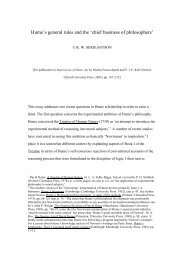
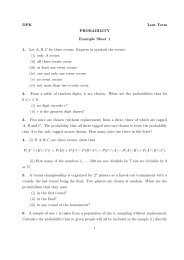
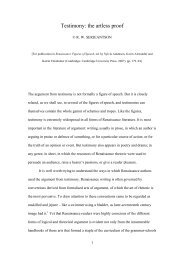
<strong>Interface</strong> <strong>circuit</strong> <strong>diagram</strong><br />
GPS requires: 4.0-5.5Vdc (60mA)<br />
(red) Vin<br />
(2x black) GND<br />
(green) RCV<br />
(white) TXD<br />
(yellow) PPS<br />
5<br />
3<br />
2<br />
1<br />
DB-9 serial connector<br />
(female)<br />
5-pin DIN<br />
20k<br />
+5V<br />
59k<br />
30k<br />
0V<br />
2.5V (*)<br />
30k<br />
V+<br />
680<br />
0.1uF<br />
150k<br />
2.5V (*)<br />
LM324<br />
1M<br />
PPS<br />
out<br />
20k<br />
2N3904<br />
Jumper to adjust gain: 0.4 open, 0.1 closed<br />
20k<br />
IR Sensor input<br />
59k<br />
3.5mm stero jack<br />
SIGNAL<br />
+5V<br />
0.1uF<br />
150k<br />
V+<br />
2.5V (*)<br />
680<br />
LM324<br />
1M<br />
IR<br />
out<br />
GND<br />
20k<br />
2N3904<br />
BNC<br />
Notes:<br />
1. The filtered outputs are intended to be connected to the datalogger. The square wave outputs<br />
should be used with a soundcard because it has its own filtering.<br />
2. The PPS signal rises to indicate the start of each second, but because of the inverting amplifier<br />
this corresponds to a falling edge in the filtered output.<br />
FIGURE A.1: <strong>Interface</strong> <strong>circuit</strong>, providing power supply to GPS and IR sensor, high-pass filtering<br />
and serial interface to GPS.<br />
42
B<br />
Derivation of the period of a non-linear pendulum<br />
The equation of motion of a pendulum is<br />
¨θ + ω 2 0 sin θ = 0<br />
(B.1)<br />
where ω 2 = g/L. For small oscillations, sin θ ≈ θ and the motion is harmonic with angular<br />
0<br />
frequency ω 0 . If the angle of swing is not small, the angular frequency will become ω, but<br />
as a first approximation the motion can still be assumed to be sinusoidal, so θ ≈ Asin ωt.<br />
Going back to the equation of motion (B.1), the sin θ term may be expanded to give<br />
<br />
¨θ + ω 2 θ − θ <br />
3<br />
0<br />
6 + . . . = 0 (B.2)<br />
<br />
<br />
−Aω 2 sin ωt + ω 2 Asin ωt − A3 sin 3 ωt<br />
+ . . . = 0 (B.3)<br />
0<br />
6<br />
sin 3 ωt may be expanded as a Fourier series:<br />
sin 3 ωt = a 1 sin ωt + a 2 sin 2ωt + . . .<br />
where the Fourier coefficients a n are given by<br />
a n = 2 π<br />
ˆ π<br />
0<br />
f (θ) sin(nθ) dθ<br />
∴<br />
a 1 = 2 π<br />
ˆ π<br />
0<br />
sin 4 ωt dt = 2 π · 3π 8 = 3 4<br />
∴ sin 3 ωt = 3 sin ωt + . . . (B.4)<br />
4<br />
So, putting (B.4) into (B.3), the approximate equation of motion is<br />
<br />
<br />
−Aω 2 sin ωt + ω 2 Asin ωt − A3 3 sin ωt · ≈ 0<br />
0<br />
6 4<br />
And hence, since T = 2π/ω,<br />
∴ ω 2 ≈ ω 2 0<br />
<br />
1 − A2<br />
8<br />
<br />
T ≈ T 0 1 + A2<br />
16<br />
<br />
(B.5)<br />
(B.6)<br />
43
C<br />
Temperature compensation<br />
C.1 Response to ramp input<br />
Using the model of a temperature compensated pendulum shown in Figure 4.4, we can<br />
derive the response of the pendulum to a transient change in temperature, for example a<br />
ramp. Assume that this change in ambient temperature affects the temperature of the outer<br />
layer T 1 directly, so the input is<br />
T 1 = T 0 + dT 1<br />
d t t<br />
If the layers are linked by a thermal resistance R, and have heat capacity mc p , the heat flow<br />
between them is<br />
Q = T 1 − T 2<br />
R<br />
and the heat flow into the inner layer is<br />
Equating these gives the governing equation:<br />
τ d T 2<br />
d t + T 2 = T 1<br />
Q = mc p<br />
dT 2<br />
d t<br />
where τ = mc p R<br />
which can be solved (e.g. by Laplace transforms) to give the response to a ramp in T 1 ,<br />
T 2 = d T 1<br />
d t<br />
<br />
(t − τ) + τe<br />
−t/τ<br />
+ T0<br />
Thus the temperature difference, once steady state is reached, is<br />
C.2 Estimation of constants<br />
T 1 − T 2 = τ dT 1<br />
d t<br />
The steel (density 7800 kg/m 3 , heat capacity 460 J/kgK, expansion coefficient 13×10 −6 K −1 )<br />
outer layer of the pendulum is approximately 35mm diameter, 2.2m long and 3mm thick.<br />
Its mass is<br />
m = ρπdl t = 5.7 kg<br />
The thermal resistance R consists of the surface convection resistances (very variable,<br />
but say 1 about 0.2 mK/W) and the air itself (conductivity 2 0.0257 W/mK). The air gap is<br />
approximately 1mm, giving<br />
Resistivity 1 1 × 10⁻³<br />
= 2 × 0.2 +<br />
U 0.0257 = 0.44 m2 K/W<br />
1 from 4D11 Building Physics notes<br />
2 from http://www.engineeringtoolbox.com/<br />
44
=⇒ Resistance R = 1<br />
UA = 0.44<br />
= 2.3 K/W<br />
π × 28 × 10 −3 × 2.2<br />
So the time constant is<br />
τ = mc p R = 5.7 × 460 × 2.0 = 6030 seconds ≈ 1.5 hours<br />
The steady temperature difference is given by<br />
so the change in going caused by this is<br />
T 1 − T 2 = τ dT 1<br />
d t<br />
∆G = −∆T<br />
T<br />
= −ατ<br />
2<br />
= −k dT 1<br />
d t<br />
= −1<br />
2 · ∆L<br />
L = −α 2 (T 1 − T 2 )<br />
dT 1<br />
d t<br />
=⇒ k = 1 2 · 13 × 10−6 · 6030 ≈ 40 ms/degree<br />
D<br />
Derivation of gravitational effects<br />
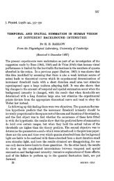
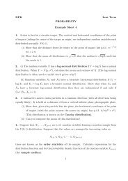
Consider first the effect of the Moon alone; the derivation below applies equally to the<br />
effect of the Sun. The are two relevant forces which act on an object on the Earth: the<br />
gravitational pull of the Moon, and the D’Alembert force corresponding to the centripetal<br />
acceleration of the Earth’s orbit with the Moon.<br />
n<br />
P<br />
F<br />
Earth<br />
R<br />
φ<br />
Ω<br />
N<br />
i<br />
Rn − ri<br />
Moon<br />
r 1<br />
r<br />
FIGURE D.1: Plan view of Earth and Moon: points F, N and P lie on the equator.<br />
45
Gravitational pull Using Newton’s Law of Gravitation, F = GM m/r 2 , the force felt by a<br />
point on the Earth varies with the inverse square of distance. As a vector, the force felt by<br />
an object of unit mass at point P is<br />
GM −(Rn − ri)<br />
F = ·<br />
2<br />
|Rn − ri| |Rn − ri|<br />
and using the cosine rule,<br />
|Rn − ri| 2 = R 2 + r 2 − 2rR cos φ<br />
so<br />
F =<br />
−GM(Rn − ri)<br />
R 2 + r 2 − 2rR cos φ 3/2<br />
If R ≪ r, then we can use the binomial expansion to give<br />
<br />
R 2 + r 2 − 2rR cos φ <br />
−3/2<br />
≈ r −3 1 − 3 <br />
R<br />
2<br />
2 r − 2R 2 r cos φ<br />
<br />
= r −3 1 + 3 R <br />
r cos φ + O ( R /r) 2<br />
We are interested in the downwards force, which is given by<br />
F · (−n) = GM <br />
1 + 3 R R<br />
r 3 r cos φ <br />
− r cos φ + O ( R/r) 2<br />
= GM <br />
R<br />
r 2 r − cos φ − 3R r cos2 φ + O ( R /r) 2<br />
≈<br />
−GM 1 R<br />
r 2 2 r + cos φ + 3 <br />
R<br />
2 r cos 2φ<br />
(since n · i = cos φ).<br />
Centrifugal force<br />
Since the Earth and Moon are orbiting each other, about a centre of<br />
rotation (the “barycentre”) located somewhere between them, the gravitational force between<br />
them must balance the centrifugal force of their rotation, i.e.<br />
F = GM eM m<br />
r 2 = M e r 1 Ω 2 = M m r 2 Ω 2<br />
=⇒ r 1 Ω 2 = GM m<br />
r 2<br />
Now consider the point P, whose position relative to the barycentre is<br />
r P = Rn − r 1 i<br />
=⇒ ¨r P = −Ω 2 Rn + Ω 2 r 1 i = −Ω 2 r P<br />
∴ D’Alembert force F = mΩ 2 r P<br />
46
So the downwards force experienced by an object of unit mass at P is<br />
Total force<br />
Ω 2 r P · (−n) = −Ω 2 R − r 1 cos φ <br />
= r 1 Ω 2 <br />
cos φ − R r 1<br />
<br />
= GM m<br />
r 2<br />
<br />
cos φ − R r 1<br />
<br />
So, the total downwards force per unit mass is<br />
<br />
R<br />
r cos 2φ + GM m<br />
r 2<br />
F down = −GM <br />
m 1 R<br />
r 2 2 r + cos φ + 3 2<br />
= −GM <br />
m 1 R<br />
r 2 2 r + 3 R<br />
2 r cos 2φ + R <br />
r 1<br />
= −1<br />
2 · GM m R<br />
1 + 3 cos 2φ + r <br />
r 2 r<br />
r 1<br />
<br />
cos φ − R r 1<br />
<br />
A downwards force per unit mass is effectively a change in gravity, so taking ∆g = F down<br />
and g = (GM e )/R 2 ,<br />
∆g<br />
g<br />
= R2<br />
× −GM <br />
mR<br />
1 + 3 cos 2φ + r <br />
GM e r 3<br />
r 1<br />
= M <br />
m R 3 1 + 3 cos 2φ + r <br />
M e r<br />
r 1<br />
Finally, the barycentre (which is the centre of mass of the Earth-Moon system) can be<br />
located by considering ‘moments of mass’ around the Earth:<br />
r 1 (M m + M e ) = r M m =⇒ r = M m + M e<br />
= λ + 1<br />
r 1 M m λ<br />
where λ = M m /M e . So<br />
∆g<br />
g<br />
R 3 <br />
= λ 1 + 3 cos 2φ + λ + 1 <br />
r λ<br />
R 3<br />
<br />
= 1 + 2λ + 3λ cos 2φ<br />
r<br />
The change in gravity due to the Moon is superimposed on that due to the Sun, to give the<br />
beating effect shown in Figure 4.5.<br />
E<br />
Risk assessment retrospective<br />
This project is almost entirely computer-based, and no specific hazards were identified apart<br />
from the usual hazards of such work. These were addressed by ensuring computer working<br />
areas were arranged comfortably, and in retrospect this seems to have been an appropriate<br />
assessment.<br />
47