indefinite integration as the reverse of differentiation
indefinite integration as the reverse of differentiation
indefinite integration as the reverse of differentiation

Create successful ePaper yourself
Turn your PDF publications into a flip-book with our unique Google optimized e-Paper software.
Integration <strong>as</strong> <strong>the</strong><br />
<strong>reverse</strong> <strong>of</strong><br />
<strong>differentiation</strong><br />
By now you will be familiar with differentiating common functions and will have had <strong>the</strong> opportunity<br />
to practice many techniques <strong>of</strong> <strong>differentiation</strong>. In this unit we carry out <strong>the</strong> process<br />
<strong>of</strong> <strong>differentiation</strong> in <strong>reverse</strong>. That is, we start with a given function, f(x) say, and <strong>as</strong>k what<br />
function or functions, F(x), would have f(x) <strong>as</strong> <strong>the</strong>ir derivative. This leads us to <strong>the</strong> concepts<br />
<strong>of</strong> an antiderivative and <strong>integration</strong>.<br />
In order to m<strong>as</strong>ter <strong>the</strong> techniques explained here it is vital that you undertake plenty <strong>of</strong> practice<br />
exercises so that <strong>the</strong>y become second nature.<br />
After reading this text, and/or viewing <strong>the</strong> video tutorial on this topic, you should be able to:<br />
• understand what is meant by <strong>the</strong> antiderivative, F(x), <strong>of</strong> a function f(x)<br />
• calculate some antiderivatives by using a table <strong>of</strong> derivatives<br />
• calculate some antiderivatives by using a table <strong>of</strong> antiderivatives<br />
• understand <strong>the</strong> link between antiderivatives and definite integrals<br />
• calculate simple definite integrals using antiderivatives<br />
• calculate simple <strong>indefinite</strong> integrals.<br />
Contents<br />
1. Introduction 2<br />
2. Antiderivatives - <strong>differentiation</strong> in <strong>reverse</strong> 2<br />
3. The link with <strong>integration</strong> <strong>as</strong> a summation 4<br />
4. Indefinite integrals 7<br />
1 c○ mathcentre August 28, 2004
1. Introduction<br />
By now you will be familiar with differentiating common functions and will have had <strong>the</strong> opportunity<br />
to practice many techniques <strong>of</strong> <strong>differentiation</strong>. In this unit we carry out <strong>the</strong> process<br />
<strong>of</strong> <strong>differentiation</strong> in <strong>reverse</strong>. That is, we start with a given function, f(x) say, and <strong>as</strong>k what<br />
function or functions, F(x), would have f(x) <strong>as</strong> <strong>the</strong>ir derivative. This leads us to <strong>the</strong> concepts<br />
<strong>of</strong> an antiderivative and <strong>integration</strong>.<br />
An earlier unit, Integration <strong>as</strong> summation, explained <strong>integration</strong> <strong>as</strong> <strong>the</strong> process <strong>of</strong> adding rectangular<br />
are<strong>as</strong>. To evaluate integrals defined in this way it w<strong>as</strong> necessary to calculate <strong>the</strong> limit<br />
<strong>of</strong> a sum - a process which is cumbersome and impractical. In this unit we will see how integrals<br />
can be found by reversing <strong>the</strong> process <strong>of</strong> <strong>differentiation</strong> - that is by finding antiderivatives.<br />
2. Antiderivatives <strong>differentiation</strong> in <strong>reverse</strong>.<br />
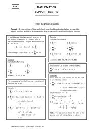
Consider <strong>the</strong> function F(x) = 3x 2 + 7x − 2. Suppose we write its derivative <strong>as</strong> f(x), that is<br />
f(x) = dF . You already know how to find this derivative by differentiating term by term to<br />
dx<br />
obtain f(x) = dF = 6x + 7. This process is illustrated in Figure 1.<br />
dx<br />
differentiate<br />
F(x) = 3x 2 + 7x − 2 f(x) = 6x + 7<br />
antidifferentiate<br />
Figure 1. The function F(x) is an antiderivative <strong>of</strong> f(x)<br />
Suppose now that we work back to front and <strong>as</strong>k ourselves which function or functions could<br />
possibly have 6x + 7 <strong>as</strong> a derivative. Clearly, one answer to this question is <strong>the</strong> function<br />
3x 2 + 7x − 2. We say that F(x) = 3x 2 + 7x − 2 is an antiderivative <strong>of</strong> f(x) = 6x + 7.<br />
There are however o<strong>the</strong>r functions which have derivative 6x + 7. Some <strong>of</strong> <strong>the</strong>se are<br />
3x 2 + 7x + 3, 3x 2 + 7x, 3x 2 + 7x − 11<br />
The re<strong>as</strong>on why all <strong>of</strong> <strong>the</strong>se functions have <strong>the</strong> same derivative is that <strong>the</strong> constant term disappears<br />
during <strong>differentiation</strong>. So, all <strong>of</strong> <strong>the</strong>se are antiderivatives <strong>of</strong> 6x+7. Given any antiderivative<br />
<strong>of</strong> f(x), all o<strong>the</strong>rs can be obtained by simply adding a different constant. In o<strong>the</strong>r words, if<br />
F(x) is an antiderivative <strong>of</strong> f(x), <strong>the</strong>n so too is F(x) + C for any constant C.<br />
Example<br />
(a) Differentiate F(x) = 4x 3 − 7x 2 + 12x − 4 to find f(x) = dF<br />
dx .<br />
(b) Write down several antiderivatives <strong>of</strong> f(x) = 12x 2 − 14x + 12.<br />
c○ mathcentre August 28, 2004 2
Solution<br />
(a) Differentiating F(x) = 4x 3 − 7x 2 + 12x − 4 we find f(x) = dF<br />
dx = 12x2 − 14x + 12. We can<br />
deduce from this that an antiderivative <strong>of</strong> 12x 2 − 14x + 12 is 4x 3 − 7x 2 + 12x − 4.<br />
(b) All o<strong>the</strong>r antiderivatives <strong>of</strong> f(x) will take <strong>the</strong> form F(x) + C where C is a constant. So, <strong>the</strong><br />
following are all antiderivatives <strong>of</strong> f(x):<br />
4x 3 − 7x 2 + 12x − 4, 4x 3 − 7x 2 + 12x − 10, 4x 3 − 7x 2 + 12x, 4x 3 − 7x 2 + 12x + 3<br />
From <strong>the</strong>se examples we deduce <strong>the</strong> following important observation.<br />
Key Point<br />
A function F(x) is an antiderivative <strong>of</strong> f(x) if dF<br />
dx = f(x).<br />
If F(x) is an antiderivative <strong>of</strong> f(x) <strong>the</strong>n so too is F(x) + C for any constant C.<br />
We can deduce many antiderivatives that we will need simply by reading a table <strong>of</strong> derivatives<br />
from right to left, instead <strong>of</strong> from left to right. However, in practice tables <strong>of</strong> antiderivatives are<br />
commonly available such <strong>as</strong> that shown in Table 1.<br />
f(x)<br />
F(x), an antiderivative <strong>of</strong> f(x)<br />
Exercises 1.<br />
k constant<br />
kx + C<br />
x 2<br />
x<br />
2 + C<br />
x 2 x 3<br />
3 + C<br />
x n x n+1<br />
(n ≠ −1)<br />
n + 1 + C<br />
sin mx<br />
− 1 m cosmx + C<br />
1<br />
cosmx<br />
sin mx + C<br />
m<br />
e mx 1<br />
m emx + C<br />
Table 1. Table <strong>of</strong> some common antiderivatives<br />
Use <strong>the</strong> Table <strong>of</strong> antiderivatives to find F(x) given f(x):<br />
1. f(x) = 5 2. f(x) = x 8 3. f(x) = 1 x 2<br />
4. f(x) = e 3x 5. f(x) = e −2x 6. cos 1 2 x.<br />
3 c○ mathcentre August 28, 2004
3. The link with <strong>integration</strong> <strong>as</strong> a summation<br />
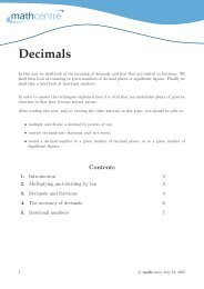
Consider that portion <strong>of</strong> <strong>the</strong> graph <strong>of</strong> y = f(x) to <strong>the</strong> right <strong>of</strong> <strong>the</strong> y axis <strong>as</strong> illustrated in Figure<br />
2. Suppose f(x) lies entirely above <strong>the</strong> x axis. Clearly <strong>the</strong> area bounded by <strong>the</strong> graph and <strong>the</strong><br />
x axis will depend upon how far to <strong>the</strong> right we move. That is <strong>the</strong> area, A, will depend upon<br />
<strong>the</strong> value <strong>of</strong> x, A = A(x).<br />
y = f(x)<br />
y<br />
A(x)<br />
x<br />
x<br />
Figure 2. The area bounded by <strong>the</strong> graph will depend upon how far to <strong>the</strong> right we move, that is A = A(x).<br />
Suppose we consider <strong>the</strong> additional contribution made to this area by moving a little fur<strong>the</strong>r to<br />
<strong>the</strong> right <strong>as</strong> shown in Figure 3. Let this additional contribution be denoted by δA. Then δA is<br />
<strong>the</strong> change in area produced by incre<strong>as</strong>ing x by δx. Note <strong>the</strong>n that δA = A(x + δx) − A(x).<br />
y<br />
y = f(x)<br />
A(x)<br />
δA<br />
δx<br />
x<br />
x<br />
Figure 3. The additional contribution to <strong>the</strong> area is δA ≈ f(x) δx.<br />
This additional contribution, δA, can be approximated by <strong>as</strong>suming it h<strong>as</strong> <strong>the</strong> form <strong>of</strong> a rectangle<br />
<strong>of</strong> height y = f(x) and width δx, that is<br />
that is<br />
In <strong>the</strong> limit <strong>as</strong> δx tends to zero we have<br />
δA ≈ f(x)δx<br />
δA<br />
δx ≈ f(x)<br />
dA<br />
dx = f(x)<br />
We can use <strong>the</strong> previous section to interpret this result.<br />
Given that f(x) is <strong>the</strong> derivative <strong>of</strong> A(x) <strong>the</strong>n, A(x) must be an antiderivative <strong>of</strong> f(x), i.e.<br />
A(x) = F(x) + C (1)<br />
In Section 2 we wrote F(x) + C for a whole family <strong>of</strong> functions all <strong>of</strong> which are antiderivatives<br />
when F(x) is. Now, we are looking for a specific antiderivative by choosing a specific value for<br />
C. This is obtained by noting that when x = 0 <strong>the</strong> area bounded is zero, that is 0 = F(0) + C,<br />
and this gives us a value for C, that is C = −F(0).<br />
We can use this result <strong>as</strong> follows: given a function f(x), <strong>the</strong>n <strong>the</strong> formula in Equation 1 can tell<br />
us <strong>the</strong> area under <strong>the</strong> graph provided we can calculate an antiderivative F(x).<br />
c○ mathcentre August 28, 2004 4
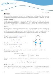
Suppose now we want to find <strong>the</strong> area under <strong>the</strong> graph between x = a and x = b <strong>as</strong> shown in<br />
Figure 4.<br />
The total area up to x = b is given, using Equation 1, by<br />
A(b) = F(b) + C<br />
The total area up to x = a is given, using Equation 1, by<br />
A(a) = F(a) + C<br />
And so, subtracting, <strong>the</strong> area between a and b is<br />
A(b) − A(a) = F(b) − F(a)<br />
Note how <strong>the</strong> C’s cancel out.<br />
y<br />
y = f(x)<br />
a<br />
b<br />
x<br />
Figure 4. The area between a and b is A(b) − A(a).<br />
Key Point<br />
When f(x) lies entirely above <strong>the</strong> x axis between a and b we can find <strong>the</strong> area under y = f(x)<br />
between a and b by finding an antiderivative F(x), and evaluating this at x = a and at x = b.<br />
The area is <strong>the</strong>n<br />
A = F(b) − F(a)<br />
In <strong>the</strong> unit entitled Integration <strong>as</strong> a summation we looked at how <strong>the</strong> area under a curve<br />
could be found by adding <strong>the</strong> are<strong>as</strong> <strong>of</strong> rectangular elements. It w<strong>as</strong> shown that <strong>the</strong> area under<br />
y = f(x) between x = a and x = b is found from<br />
This limiting process is denoted by<br />
A = lim<br />
δx→0<br />
x=b<br />
∑<br />
f(x) δx<br />
x=a<br />
A =<br />
∫ b<br />
a<br />
f(x) dx<br />
and this defines what we mean by <strong>the</strong> definite integral <strong>of</strong> f(x) between <strong>the</strong> limits a and b.<br />
5 c○ mathcentre August 28, 2004
So we now have two ways <strong>of</strong> finding <strong>the</strong> area under a curve, one involving taking <strong>the</strong> limit <strong>of</strong><br />
a sum, that is finding a definite integral, and one involving find an antiderivative. Generally,<br />
finding <strong>the</strong> limit <strong>of</strong> a sum is difficult, where<strong>as</strong> with some practice, finding an antiderivative is<br />
much simpler. So, in future we can avoid <strong>the</strong> more difficult way and evaluate integrals using<br />
antiderivatives.<br />
Key Point<br />
If F(x) is any antiderivative <strong>of</strong> f(x) <strong>the</strong>n<br />
∫ b<br />
a<br />
f(x)dx = F(b) − F(a)<br />
Example<br />
∑x=1<br />
Suppose we wish to evaluate lim x 2 δx. This limit <strong>of</strong> a sum arises when we use <strong>the</strong> sum <strong>of</strong><br />
δx→0<br />
x=0<br />
small rectangles to find <strong>the</strong> area under y = x 2 between x = 0 and x = 1. This limit defines <strong>the</strong><br />
definite integral<br />
∫ 1<br />
0<br />
x 2 dx<br />
Using <strong>the</strong> Key Point above we can evaluate this integral by finding an antiderivative <strong>of</strong> x 2 . This<br />
is F(x) = x3<br />
+ C. We evaluate this at x = 1 and x = 0 and find <strong>the</strong> difference between <strong>the</strong> two<br />
3<br />
results:<br />
∫ 1<br />
( ) ( )<br />
1<br />
x 2 3<br />
0<br />
3<br />
dx =<br />
3 + C −<br />
3 + C<br />
0<br />
= 1 3<br />
Note that <strong>the</strong> C’s cancel - this will always happen, and so in future when dealing with definite<br />
integrals we will omit <strong>the</strong> C altoge<strong>the</strong>r. It is conventional to set <strong>the</strong> previous calculation out <strong>as</strong><br />
follows:<br />
∫ 1<br />
[ ] x<br />
x 2 3 1<br />
dx =<br />
0 3<br />
0<br />
( ) ( )<br />
1<br />
3 0<br />
3<br />
= −<br />
3 3<br />
= 1 3<br />
More generally we write<br />
∫ b<br />
a<br />
f(x)dx = [F(x)] b a<br />
= F(b) − F(a)<br />
c○ mathcentre August 28, 2004 6
Exercises 2<br />
Evaluate <strong>the</strong> following limits <strong>of</strong> sums using antiderivatives.<br />
∑<br />
1. Find lim x 3 δx.<br />
2. Find lim<br />
3. Find lim<br />
x=1<br />
δx→0<br />
x=0<br />
∑x=2<br />
δx→0<br />
x=1<br />
∑x=1<br />
δx→0<br />
x=0<br />
x 4 δx.<br />
e 2x δx.<br />
4. Indefinite integrals<br />
As we have seen definite <strong>integration</strong> is closely <strong>as</strong>sociated with finding antiderivatives. Because<br />
<strong>of</strong> this it is common to think <strong>of</strong> anti<strong>differentiation</strong> in general <strong>as</strong> <strong>integration</strong>. So when <strong>as</strong>ked to<br />
<strong>reverse</strong> <strong>the</strong> process <strong>of</strong> <strong>differentiation</strong> this is commonly referred to <strong>as</strong> <strong>integration</strong>.<br />
In <strong>the</strong> Example on page 2 we found antiderivatives <strong>of</strong> f(x) = 12x 2 −14x+12. Using <strong>integration</strong><br />
notation we would commonly write<br />
∫<br />
(12x 2 − 14x + 12)dx = 4x 3 − 7x 2 + 12x + C<br />
and refer to this <strong>as</strong> <strong>the</strong> <strong>indefinite</strong> integral <strong>of</strong> 12x 2 − 14x + 12 with respect to x. The constant<br />
C is called <strong>the</strong> constant <strong>of</strong> <strong>integration</strong>. Tables <strong>of</strong> antiderivatives such <strong>as</strong> Table 1 are <strong>of</strong>ten<br />
called Tables <strong>of</strong> Integrals.<br />
Key Point<br />
∫<br />
The <strong>indefinite</strong> integral <strong>of</strong> <strong>the</strong> function f(x), f(x)dx, is ano<strong>the</strong>r function. It is given by<br />
F(x) + C where F(x) is any antiderivative <strong>of</strong> f(x) and C is an arbitrary constant.<br />
The definite integral <strong>of</strong> <strong>the</strong> function f(x) between <strong>the</strong> limits a and b,<br />
∫ b<br />
a<br />
f(x)dx, is a number.<br />
It may be obtained from <strong>the</strong> formula F(b) − F(a), where F(x) is any antiderivative <strong>of</strong> f(x).<br />
In this unit we have described how to carry out <strong>differentiation</strong> in <strong>reverse</strong>, leading to <strong>the</strong> concept<br />
<strong>of</strong> an antiderivative. We have also seen how we can use antiderivatives to find integrals. In<br />
subsequent units you can learn how to integrate a much wider range <strong>of</strong> functions that are met<br />
in engineering and <strong>the</strong> physical sciences.<br />
7 c○ mathcentre August 28, 2004
Exercises 3.<br />
Use a Table to find <strong>the</strong> following integrals:<br />
∫ ∫<br />
∫<br />
1. e 2x dx 2. sin 3x dx 3. cos 7x dx<br />
4.<br />
∫<br />
Answers<br />
e −3x dx 5.<br />
Exercises 1.<br />
∫ 1<br />
x 3 dx<br />
6. ∫<br />
x 1/2 dx<br />
1. 5x + C 2. x9<br />
9 + C 3. −1 x + C<br />
4. 1 3 e3x + C 5. − 1 2 e−2x + C 6. 2 sin 1 2 x + C.<br />
Exercises 2.<br />
1. 1 2. 31<br />
4 5<br />
Exercises 3.<br />
3. 1 2 (e2 − 1).<br />
1. 1 2 e2x + C 2. − 1 3 cos 3x + C 3. 1 sin 7x + C<br />
7<br />
4. − 1 3 e−3x + C 5. − 1 2x3/2<br />
+ C 6. + C.<br />
2x2 3<br />
c○ mathcentre August 28, 2004 8