Final Exam

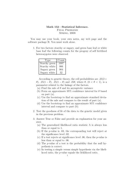
Math 152—Statistical Inference.
Final Problems
Spring, 2008
You may use your book, your own notes, my web page and the
software package R. You must work alone.
1. For two factors–starchy or sugary, and green base leaf or white
base leaf–the following counts for the progeny of self fertilized
heterozygotes were observed
Type Count
Starchy green 1997
Starchy white 906
Sugary green 904
Sugary white 32
According to genetic theory, the cell probabilities are .25(2 +
θ), .25(1 − θ), .25(1 − θ) and .25θ, where θ, (0 < θ < 1), is a
parameter related to the linkage of the factors.
(a) Find the mle of θ and its asymptotic variance
(b) Form an approximate 95% confidence interval for θ based
on part (a).
(c) Use the bootstrap to find an approximate standard deviation
of the mle and compare to the result of part (a).
(d) Use the bootstrap to find an approximate 95% confidence
interval and compare to part (b).
2. Test the goodness of fit of the data to the genetic model given
in the previous problem.
3. Answer True or False and provide an explanation for your answer.
(a) The generalized likelihood ratio statistic Λ is always less
than or equal to 1.
(b) If the p-value is .03, the corresponding test will reject at
the significance level .02.
(c) If a test rejects at significance level .06, then the p-value is
less than or equal to .06.
(d) The p-value of a test is the probability that the null hypothesis
is correct.
(e) In testing a simple versus simple hypothesis via the likelihood
ratio, the p-value equals the lieklihood ratio.
1

2
(f) If a chi-square test statistic with 7 degrees of freedom has
a value of 8.5, the p-value is less than .05.
4. The intensity of light reflected by an object is measured. Suppose
there are two types of possible objects, A and B.If the
object is of type A, the measurement is normally distributed
with mean 100 and standard deviation 25; if it is of type B, the
measurement is normally distributed with mean 125 and standard
deviation 25. A single measurement is taken with value
X = 120.
(a) What is the likelihood ratio?
(b) If the prior probabilities of A and B are equal, what is the
posterior probability that the item is of type B?
(c) Suppose that a decision rule has been formulated that declares
the object to be of type B if X > 125. What is the
significance level associated with this rule?
(d) What is the power of this test?
(e) What is the p-value when X = 120?
5. Suppose that a sample is taken from a symmetric distribution
whose tails decrease more slowly than thos of the normal distribution.
What would be the qualitative shape of a normal
probability plot of this sample?
6. Suppose that F is an exponential distribution with parameter
λ = 1 and that G is exponential with parameter λ = 2. Sketch
a Q-Q plot.
7. Explain how the bootstrap could be used to approximate the
sampling distribution of the MAD.
8. Demographers often refer to the hazard function as the ”‘age
specific mortality rate,” or death rate. Until recently, most researchers
in the field of gerontology thought that a death rate
increasing with age was a universal fact in the biological world.
There has been heavy debate over whether there is a genetically
programmed upper limit to lifespan. Using a facility in
which sterelized medflies are bred to be released to fight medfly
infestation in California, investigators bred more than a million
medflies and recorded their pattern of mortality. The data file
”medflies”, available at the course web page, contains the number
of medflies alive from an initial population of 1, 203, 646 as
a function of age in days. Using these data, estimate the age

specific mortality rate. Does it increase with age? What conclusions
can you draw about the age specific mortality of the
medflies?
hints: One can approximate the derivative by 5 or 10 day
difference quotients. The R command read.csv operates exactly
as read.table.
9. In their 1994 paper, “The bone density of female twins discordant
for tobacco use” (N. Eng. J. Med., 330, 387-392), Hopper
and Seeman studied the relationship between bone density and
smoking among 41 pairs of middle-aged female twins. In each
pair, one twin was a lighter smoker and one a heavier smoker,
as measured by pack-years, the number of packages of cigarettes
consumed in a year. Bone mineral density was measured
at the lumbar spine, the femoral neck (hip), and the femoral
shaft. As well as smoking, other variables, such as alcohol consumption
and tea and coffee consumption, were recorded. The
data are contained in the file “bonden” and documentation is
in the file “bondendoc”. Use graphical methods and statistical
tests (if possible) to compare bone densities of the heavy and
light smoking twins. Do any other variables bear a relationship
to bone density? After completing your analysis, compare
your conclusions to those in the paper (which is available online
through the Claremont Colleges Library web page). Your
techniques will differ from those used by the investigators, so
do your analysis before looking at the paper.
10. The difference of the means of two normal distributions with
equal variance is to be estimated by by sampling an equal number
of observations from each distribution. If it were possible,
would it be better to halve the standard deviations of the populations
or double the sample sizes?
11. Find the exact null distribution of the Mann-Whitney Statistic,
U Y , in the case where m = 3 and n = 2.
12. An experiment was done to test a method for reducing faults
on telephone lines. Fourteen matched pairs of areas were used.
The following table shows the fault rates for the control areas
and the test areas:
3

4
Test Control
676 88
206 570
230 605
256 617
280 653
433 2913
337 924
466 286
497 1098
512 982
794 2346
428 321
452 615
512 519
(a) Plot the differences versus the control rate and summarize
what you see.
(b) Calculate the mean difference, its standard deviation, and
a confidence interval.
(c) Calculate the median difference and a confidence interval
and compare to the previous result.
(d) Do you think it is more appropriate to use a t test or a nonparametric
method to test whether the apparent difference
between test and control could be due to chance?Why?
Carry out both tests and compare.
13. The media often present short reports of the results of experiments.
To the critical reader or listener, such reports often raise
more questions than they answer. Comment on possible pitfalls
in the interpretation of each of the following.
(a) Nonsmoking wives whose husbands smoke have a cancer
rate twice that of wives whose husbands do not smoke.
(b) A 2-year study in North Carolina found that 75% of all
industrial accidents in the state happened to workers who
had skipped breakfast.
(c) A survey found that ose who drank a mderate amount of
beer were healthier than those who totally abstained from
alcohol.
(d) A University of Wisconsin study showed that within 10
years of the wedding, 38% of those who had lived together

efore marriage had split up, compared to 27% of those
who had married without a “trial”’ period.
5