Computational Astrophysics: N-Body Exercise

Computational Astrophysics: N-Body Exercise
Part 3 Laboratories
March 23, 2005
1

Contents
1 Some words about third year labs 3
2 Background 4
3 N-body Codes 4
3.1 Algorithm . . . . . . . . . . . . . . . . . . . . . . . . . . . . . . . . . . . . . . . 4
3.2 Accuracy . . . . . . . . . . . . . . . . . . . . . . . . . . . . . . . . . . . . . . . . 5
3.3 Exploring Parameter Space . . . . . . . . . . . . . . . . . . . . . . . . . . . . . 6
3.4 Units . . . . . . . . . . . . . . . . . . . . . . . . . . . . . . . . . . . . . . . . . . 6
4 The computer and the program 6
4.1 The Programming Environment . . . . . . . . . . . . . . . . . . . . . . . . . . . 6
4.2 The Program . . . . . . . . . . . . . . . . . . . . . . . . . . . . . . . . . . . . . 7
4.3 Programming Hints . . . . . . . . . . . . . . . . . . . . . . . . . . . . . . . . . . 7
5 Structure of this Exercise 7
6 Projects 9
6.1 Black Holes and the End of the Earth (Standard Exercise) . . . . . . . . . . . . 9
6.1.1 Background . . . . . . . . . . . . . . . . . . . . . . . . . . . . . . . . . . 9
6.1.2 Program . . . . . . . . . . . . . . . . . . . . . . . . . . . . . . . . . . . . 9
6.1.3 Initial Conditions . . . . . . . . . . . . . . . . . . . . . . . . . . . . . . . 10
6.1.4 Exercise . . . . . . . . . . . . . . . . . . . . . . . . . . . . . . . . . . . . 10
6.2 Binary Stars and Alien Civilisations (Advanced exercise) . . . . . . . . . . . . . 10
6.2.1 Background . . . . . . . . . . . . . . . . . . . . . . . . . . . . . . . . . . 10
6.2.2 Program . . . . . . . . . . . . . . . . . . . . . . . . . . . . . . . . . . . . 11
6.2.3 Initial Conditions . . . . . . . . . . . . . . . . . . . . . . . . . . . . . . . 11
6.2.4 Experiment . . . . . . . . . . . . . . . . . . . . . . . . . . . . . . . . . . 11
7 Numbers 12
8 Acknowledgements 13
2

1 Some words about third year labs
These notes don’t contain all the information you need - they’re here to define the terms for
you, and to give you an idea of the direction you should be taking. You’ll find that you need
to go foraging for more detailed information in other places - often in the references, and even
more often in the rubble of your demonstrators’ minds. You’re going to learn a lot while you’re
doing that, so don’t waste the effort - share all the work you’re doing with us in your report!
Remember that your report has to be self-contained. It doesn’t have to be beautiful, but it
should be clear and detailed. Perhaps the most important thing to remember is that when you
write your report you’re trying to teach your reader what you did, why you did it, and what
you learned. That way, we get to learn something too! Enjoy!
By the way, these notes have recenlty undergone a major revision, and may be littered with typos
(and possibly more serious errors). We in part3 would love it if you could bring any mistakes
to the attention of your demonstrators, or email suggestions to part3@physics.unimelb.edu.au
3

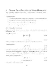
2 Background
It is a remarkable and sobering thought that it is impossible to solve the equations for three
or more bodies flying around in space under the influence of their mutual gravity. In special
cases you can make useful approximations, but in general, the problem is insoluble.
This is a major menace in astronomy, which after all is the study of large numbers of objects
flying around in space under the influence of gravity.
In the late 18th century, a partial solution was found. While it is impossible to calculate
the orbits exactly, you can calculate a really good approximation valid for a short period of
time. You start by putting all your bodies in their starting positions. You then work out the
gravitational force on each object at this time. Using this force, you work out the acceleration
on each body. Using this acceleration, you work out the velocity of each body. Using this
velocity, you work out where each body will be a short time in the future. You move each body
to its new position. You then go through the whole process again, starting at the new position.
In this slow, painful, tedious way, you can calculate even the most complex situations. Thousands
of calculations were required. Teams of students would sit at rows of desk, each calculating
one tiny stage over and over again for long years. But the rewards were great – it was from
calculations such as these that the planet Neptune was discovered.
Luckily for you, computers were invented. They are perfectly suited for this job; computers
love nothing more than doing simple calculations over and over again. In this exercise, you will
use a computer program that will do in seconds the same calculations that took some of the
greatest astronomers of the last century most of their lives.
3 N-body Codes
The program you will be working with is one of a class of programs called n-body codes. They
deal with a number of small, well separated objects, moving under the influence of their mutual
gravitational attraction. Assume throughout that all the objects can be treated as points; for
example if the Earth is in orbit around the Sun, assume that all the mass of the Sun is at the
centre of the Sun for calculation purposes.
Warning! Do not attempt to solve the equations on paper – there is no general solution to
the three-body code, and even limited, special-case solutions are hair-raisingly difficult. If you
find yourself writing down pages of equations, you’re doing this the wrong way. All the maths
you need can be written in about three lines!
3.1 Algorithm
How can we simulate particles moving in orbit around each other? The physics is simple; we
use Newton’s inverse square law of Gravity,
F = GM 1M 2
r 2 (1)
4

where F is the force, G = 6.67 × 10 −11 Nm 2 kg −2 , and r the distance between the two objects.
We proceed as follows:
1. We choose initial positions and velocities for all our objects.
2. Using Newton’s law (above) we work out the force on each object due to the gravitational
attraction of the others. The force is a vector quantity, and as gravity is linear, the total
force on each object is the vector sum of the forces on it due to each of the other bodies.
3. Using the force we just calculated, we work out the acceleration of the body.
4. We now take a small step forward in time, and compute the new position and velocity
of all the objects. The new position is simply the old position plus the product of the
velocity and the time step. The new velocity is the old velocity plus the product of the
acceleration and the time step.
5. Repeat steps 2—4.
Simple! The key to computer programming is to remember that computers are pretty stupid.
They can only do simple things, but they do them very fast. Break your problem into tiny
little pieces, and get the computer to do them one after another very fast.
3.2 Accuracy
“How big should our time step be?”. “How long should we run our code for?”. These are the
most common questions demonstrators get asked, and there is no easy answer.
You run your code for as long as it takes to answer the astronomical problem. But your code
isn’t precise – you had to make approximations to solve the three-body problem, and the
longer you run your code for the worse these approximations get. The smaller your time-step,
the smaller the errors, but the slower your code – you must compromise.
In the algorithm above, you’ve approximated the true curvy orbit of the bodies with a series
of straight lines. Every time you take a step, this means you will be slightly in error, and these
tiny errors can build up until your program gives you complete garbage.
You should work out how big this error will be. You can do this mathematically, but a more
immediate way to estimate this is to simulate a situation you know. For example, simulate the
Earth going round the Sun. If your program doesn’t put the Earth in orbit with a period of
about a year, your code is wrong. But check – does the radius of the orbit remain constant?
Does the period remain constant? If not, how big is the error? Is it systematic? How long does
it take for the error to get big? Does it depend on the size of the time steps you use?
These errors will determine how good your simulation will be. If, for example, after 20 orbits
your program has changed the Earth’s orbit by 10%, you certainly couldn’t trust your program
to accurately predict the position of a spacecraft after 20 orbits. Marks will be awarded for
how well you estimate your errors, and how carefully you take them into account in carrying
out your research project.
5

If you make your time step smaller, your program will be more accurate. This however will
slow down the computer, so you won’t be able to run as many simulations, or to run them for
as long. You will have to make your own decision on the trade-off between small time-steps
and a comprehensive exploration of the parameter space (below).
What will happen if your objects get close to each other? If the distance they travel in a time
step is comparable to the distance between two objects, you’ve got trouble (why?). There are
ways to fix this in the code, but the simplest way out is not to let the objects get this close; if
you have to have close encounters in your simulation, use very small time steps.
For advanced students: there is a simple modification you can make to the above program to
greatly reduce systematic errors. . .
3.3 Exploring Parameter Space
In all the projects below, you have a wide choice of free parameters. What are the starting
masses? What are the starting positions and speeds? You may feel that you have been given
far too little guidance about these things. You are right, and this is a problem professional
astronomers face all the time. For example, at the moment I am trying to simulate the formation
of a galaxy. I’m asking questions like “what should I use as the building blocks?”, “how hot
will the building blocks be?”, “how fast are they moving?”. There are no definite answers.
What you have to do is explore parameter space. There will be some plausible range of input
parameters. Explore it! Try out different values; home in on the most interesting ones. This is
an important and difficult skill, and a lot of marks will depend on how well you do it.
3.4 Units
You are probably used to working in S.I. units. These are fine for things of order 1m long (like
you and me), but for your average star (mass ∼ 10 30 kg), you’ve got problems. Most computers
can handle numbers as large as 10 ±34 , but all you would need to do is multiply the mass of the
Earth and the Sun together, and the program would crash.
The simplest solution is to invent new units for mass, length and time. If you choose these
units correctly, your program will be dealing with numbers like 1, rather than 10 30 .
4 The computer and the program
4.1 The Programming Environment
The computer for this lab uses Windoze 98 and a graphical C compiler. Create a directory for
yourself under the “D:/student/” directory.
6

4.2 The Program
A template program “D:/student/nbody.cpp” has been provided for you. Make a copy of this
program in your directory. This has the basic n-body code, that will calculate the positions
and velocities of the bodies for a given number of time-steps. This has been provided so that
you can concentrate more on the actual science involved, rather than spending most of your
time writing programs. You will, however, need to do a little bit programming, to calculate
things like the total energy of the system, and the planetary temperature and so forth. In this
case, the following section may be of some use.
4.3 Programming Hints
Talk to your demonstrators for lots of hints on good programming style. But here are a few
key hints:
1. Write out your code on paper before you type it in. The most common error novice
(and experienced) programmers make is to write half the code before realising that they
don’t really understand in detail the algorithm they are trying to code. Make sure you
are absolutely clear in your mind about what you want to do before touching finger to
keyboard.
2. Write clear, well commented code. Far more time is spent de-bugging programs than
writing them in the first place; if your code is clearly and logically laid out, with lots of
comments, it will save your hours in the long term.
3. Give your variables sensible names. If all your variables are called things like XAA you
will have to look up what they mean every time you have to alter your code, but something
called XVELOCITY is a little more obvious.
4. Test your code. No program longer than about ten lines ever works first time. If you test
each little part of your program independently, it will be much easier to debug. Also,
never believe what your program is telling you until you’ve tried it on a problem where
you know the answer.
5 Structure of this Exercise
This exercise is set up like a mini research project. You should work through the theory, and
make sure you understand what you will be modelling with the program. Next, familiarise
yourself with the n-body code provided, making sure you can get it to work. Then, read
through the two possible projects in section 6. One of these involves a more detailed analysis
and should only be attempted by those with a strong programming background.
You should go through the following steps:
• Theory section :
7

1. Write down the basic equations governing motion – those for force, acceleration and
so on. Now rewrite them using discrete time steps ∆t. These are the equations that
will be used in a computer program.
2. Now consider Newton’s equation for gravity. Write this in terms of vectors (using
⃗r 1 and ⃗r 2 as the position vectors of two particles), and separate out into x, y, and z
components.
3. Draw up a flow chart of how an N-body algorithm will work. This does not mean
write a program!!! Rather, write the steps required to calculate the necessary forces,
positions etc. at each time-step. (This should be more detailed than the basic algorithm
given in Section 3.1!)
Also, think about what units to use – for instance, what would you measure the
distance in? Why?
Wait for a demonstrator to check what you have done before continuing.
• Programming :
1. Now look at the template code that is provided on the computers. (This code is
written in the C programming language.) Match up what the code does with your
flow chart. How well do they agree? Make your own copy of the template, so that
you can alter it as you go along.
Please don’t edit the template file!
2. For your first exercise, set the Earth going around the Sun in a way that mimics
reality. What will be the initial conditions – velocities, positions?
3. Try to determine how accurate your code is. Give some thought as to how you
can work out the errors in your results, and how you can make your program more
accurate. In doing this, explore the parameter space a little and get a feel for the
range of parameters for which things still work well. Things to try would be :
– Change ∆t. (What is the physical interpretation of a large or small ∆t?)
– Change the number of orbits your Earth makes.
4. Try increasing/decreasing the initial velocity by a small amount and/or a significant
amount (order of magnitude perhaps?) – what happens? Also try a velocity close
to the escape velocity (work this out first).
5. Find a way to work out how many orbits the planet is doing. – how many orbits
can you get in a sensible time? (Make this independent of the initial parameters –
it needs to be adaptable in case the orbit changes e.g. due to the influence of a third
body.)
6. Check whether energy is being conserved by your program – what is the expression
for the total energy in the system? If conservation is not taking place, explain why.
7. Finally, convert your program to a 3-body problem by adding Jupiter to the simulation.
Check that it still works and that it gives reasonable results.
• Project work : Read both of the projects detailed below, and choose one to work on.
Restrict yourself to a 2D problem, i.e. no z-motion. Questions :
1. What are the dependent parameters?
8

2. How can you systematically explore parameter space?
3. What are realistic values for the various parameters?
See appendix for information on calculating the temperature at Earth (as this is required
for both projects). Note that the appendix calculates the temperature based on one star
– you will need to adapt this calculation if you have a binary system. How will it change?
• Discussion :
1. Write a brief summary of the results of your investigation. Make sure you answer
the aims you had at the start.
2. What happened when two bodies got too close to each other (or even had the same
position)? What does Newton’s equation predict? Is this scenario physical? (i.e. is
it likely to happen with real planets or stars?) How could you make your calculations
more realistic?
3. Did you notice any change in speed while running the program, particularly when
going from two bodies to three? Do you think this is a realistic method for n-body
simulations where n ∼ 100?
6 Projects
Pick one of these two projects. Please note that if you have little (or no) programming
experience, you are better off choosing the standard exercise.
6.1 Black Holes and the End of the Earth (Standard Exercise)
6.1.1 Background
One of the greatest mysteries of modern astronomy is the enigma of dark matter. We know
there is a lot of stuff out there that we can’t see – what we don’t know is what form it is in.
One suggestion is that the dark matter is in the form of black holes, millions of them, flying
unobserved in the dark depths of interstellar space.
What would happen if one of these hypothetical black holes wandered past our solar system?
Would it suck the Earth into its orbit and carry us away? Would it disturb our orbit and make
us fall into the sun, or fling us out into interstellar space to slowly freeze? This project aims to
find out.
6.1.2 Program
For this exercise you will need a simple 3-body code as described in section 4. The Earth’s
mass is far too small to deflect either the Sun or the Black Hole, so don’t bother calculating its
effect on them – indeed you may choose to calculate the orbits of the sun and the Black hole
rather than computing them in the program.
9

6.1.3 Initial Conditions
Start with the Earth in its usual nice steady orbit around the Sun. Fling in the black hole from
a range of directions and orientations. See what happens if it gives the Sun a near miss, or
passes by much further out.
How massive should the black hole be? If it forms from the collapse of a Supernova, it must
weight more than a mass known as the Chandrasekhar mass (stars smaller than this end up as
white dwarfs instead). This gives you the lower limit on the range of masses you should play
with. It is possible there could be black holes out there which weight as much as a thousand
times the mass of the Sun, but such massive holes should be rare. Concentrate on the effects
of smaller black holes, but run a few simulations with the really big ones just to find out what
happens.
How fast will the Black Hole approach? Stars in our part of the galaxy are typically moving
at speeds of about 200 km/s, in their orbits around the centre of our galaxy. If the black hole
were in a similar orbit to our Sun, it might sidle up relatively slowly, say 10 km/s. If however
it was rotating the other way around the galactic centre, it might be travelling at 400 km/s,
and if it was an interloper from intergalactic space, the speed might be higher still.
6.1.4 Exercise
See where the Earth ends up after each Black-hole encounter. If it ends up in orbit around the
Black hole, or flung into interstellar space, it is obviously curtains for life on Earth. But what
if it ends up in a different and/or distorted orbit around the Sun? Get your program to work
out the temperature of the Earth at each point. Assume it is a black body whose only heat
source is the Sun, and that it is in thermodynamic equilibrium. Is this assumption reasonable?
If we were flung out into interstellar space, how long would we take to cool down?
6.2 Binary Stars and Alien Civilisations (Advanced exercise)
6.2.1 Background
Is there life on other planets? The question is still wide open; we just don’t know. However,
one group of astronomers have recently argued against life in space. Their argument goes like
this:
• Our Sun is a very unusual one; most stars in the galaxy (more than 70%) are double
stars, pairs of stars orbiting each other.
• For life to evolve on a planet, it must have stable conditions for at least millions of years.
If, for example, a planet kept wandering up close to stars and far away from them again,
any life trying to evolve would be alternatively frozen and fried.
• No planet can survive in a stable orbit around a double star.
Recently, a group of astronomers claimed to have detected the presence of a planet in a double
star system, although doubt has since been thrown on these claims. The aim of this project is
10

to test this scenario. Can a planet survive in a reasonably stable orbit around a double star?
If not, will the planet be flung into deepest space or drawn in close to the central fires? How
bad will this be?
6.2.2 Program
For this, you will need a three-body program; a code capable of handling the orbits of two stars
(the binary) and one planet. By definition, planets are much smaller and lighter than stars,
so you can ignore the pull of the planet upon the stars; consider only the pull of the two stars
on the planet. You may choose to calculate the orbits of the two stars mathematically, or to
simulate it; both approaches have their advantages.
6.2.3 Initial Conditions
You should run your program with a range of initial conditions. Things to investigate include:
• The separation of the Binary stars. Binary stars can be separated by as little as an
astronomical unit and as much as half a parsec.
• What are the masses of the two stars? (The mass of the planet doesn’t matter; why
not?). Stars range in mass from 10% of the Sun’s mass to 100 times the Sun’s mass, and
there is no reason for the two stars to have the same mass.
• How far is the planet from the stars? Is it in orbit around one of them, or about the
centre of mass of the two? If it is too close, it will be too hot for life, and if it is too
far away, it will be too cold. As the aim of this project is to see if life can form, don’t
bother simulating planets too far out or too close. Assume that the planet is a black
body, and that the binary stars have luminosities roughly like that of the Sun. Using the
Stefan-Boltzmann law (and the Appendix), work out roughly the sort of distances the
planet can be from the suns while having a reasonable temperature. Bear in mind that
massive stars can be much brighter than the sun. Also note that you will need to adapt
the equations in the appendix to include the flux from the second star.
• Is the planet moving in the same direction as the stars or a different one? Does it make
a difference?
Experiment with these initial conditions. You will soon find that for most conditions, your
planet is soon fried or frozen. Concentrate on that small range of parameters that leave the
planet relatively intact. Always start the planet in a roughly circular orbit, with roughly the
right velocity to keep it there – obviously if you start the planet on an eccentric orbit it is
bound to suffer dramatic temperature variations.
6.2.4 Experiment
There won’t be a simple answer to the question “can life survive on a planet around a binary
star”. For a start, binary stars are very diverse. We don’t know what temperatures alien life
11

forms could survive or even enjoy. And given the limited accuracy of our simulation, we can’t
follow a planet for very long; even if the planet is still fine after 100 orbits (if 100 orbits is all
your program can cope with, while giving accurate answers), we don’t know that it would still
be OK after a million.
What you should say in your conclusions is something like “In these circumstances the planet
will rapidly go walkabout, its temperature rising above one zillion K. The best conditions
for life are if. . . ”. As usual in astronomy, exact answers are not needed; if you’ve gained an
understanding of the sorts of things that influence a planet’s survival, with some rough numbers,
you will have done well.
7 Numbers
• An astronomical unit (AU, the distance from the Earth to the Sun) is 1.496 × 10 11 m.
• The radius of the Earth is 6380 km
• One parsec is 3.086 × 10 16 m (3.26 light years)
• The radius of Mars is 3400 km.
• The distance between the Sun and Mars is 1.524 astronomical units
• The distance between the Sun and the Kuiper belt is between 40 and 100 astronomical
units.
• The mass of the Earth is 5.97 × 10 24 kg.
• The mass of the Sun is 2.00 × 10 30 kg.
• The mass of Mars is 6.4 × 10 23 kg.
• The Chandrasekhar mass is 1.4 times the mass of the Sun.
• The mass of a typical galaxy is 10 10 times that of the Sun.
• The luminosity of the Sun is 3.8 × 10 26 W.
• The temperature of the Sun is 5800 K.
• The radiation temperature of deep space is 2.7K.
Appendix – planetary temperatures
To calculate the temperature of a planet, we assume that both the planet and the Sun are
blackbodies, and we find the temperature at which the little blackbody must radiate to balance
the energy input from the big blackbody.
Assuming the Sun can be approximated by a blackbody, the energy flux is given by the Stefan-
Boltzmann law
F = σT 4 W m −2
12

where σ = 5.67 × 10 −8 W m −2 K −4 . This can be converted into the luminosity – the total
power output – by multiplying by the surface area of the Sun
L ⊙ = 4πR 2 ⊙ F ⊙ = 4πR 2 ⊙ σT 4 W
Since this energy all flows through a sphere of radius r p , the planet-Sun distance, the flux at
r p must be given by
F p = 4πR2 ⊙ F ⊙
4πr 2 p
= (R ⊙ /r p ) 2 F ⊙
Now, it would be possible to calculate the temperature straight from F p , which is called the
subsolar temperature. But, this is not the appropriate value for most planets, which have
atmospheres, or reasonably rapid rotation. For these, we need to calculate the equilibrium
temperature, which takes into account the energy radiated by the planet, as well as the albedo,
which is the fraction of solar radiation incident on the planet that is reflected.
The albedo is denoted by A, and if A is the fraction reflected, then 1 − A is absorbed. This
means that power absorbed by the planet is
(1 − A)πR 2 p F p = (1 − A)πR 2 p (R ⊙/r p ) 2 F ⊙
since the cross section of the planet is πR 2 p , where R p is the planet’s radius. For an equilibrium
temperature, the absorbed power must equal the radiated power, which is given by 4πR 2 pσT 4 p .
Thus, equating these two expressions, we get the temperature to be
or, expressing r p in astronomical units (AU),
T p = (1 − A) 1/4 (R ⊙ /2r p ) 1/2 T ⊙
T p ≈ 279(1 − A) 1/4 (r p ) −1/2
Note that this temperature does not take into account effects such as the heat retention of
atmospheres (e.g. greenhouse effects), internal heating of planets, or variations of A with wavelength.
Typical values of A for planets are 0.4 (Earth), 0.76 (Venus), 0.16 (Mars), and 0.51
(Jupiter).
[Adapted from Zeilik & Gregory, “Introductory Astronomy and Astrophysics”, 4th Edition, Saunders
College Publishing.]
8 Acknowledgements
Original document: Paul Francis, Chris Fluke and Matt Whiting.
Updates 2005: Randall Wayth.
13

Safety in the third year laboratory
This is to certify that the undersigned person has completed the following:
• they have read and understood the ”General Safety notes” for the overall third year
experimental laboratories;
• they have read and understood the safety notes specific to the experiment listed below;
• they have been trained in the use of specialised equipment used in this experiment by the
demonstrator listed below.
Experiment: ...................................................
Specalised equipment: ...................................................
...................................................
...................................................
...................................................
...................................................
..................................................
..................................................
Demonstrator:
.....................................................
Print name .......................................................
Signature ...................................................
Student:
Print name .......................................................
Signature ...................................................
Date: ...................................................
14