FUSION/LDV: Software for LIDAR Data Analysis and Visualization

United States
Department of
Agriculture
Forest Service
Pacific Northwest
Research Station
FUSION/LDV: Software for
LIDAR Data Analysis and
Visualization
Robert J. McGaughey
April 2008

The Forest Service of the U.S. Department of Agriculture is dedicated to the principle of
multiple use management of the Nation’s forest resources for sustained yields of wood,
water, forage, wildlife, and recreation. Through forestry research, cooperation with the
States and private forest owners, and management of the National Forests and National
Grasslands, it strives—as directed by Congress—to provide increasingly greater service
to a growing Nation.
The U.S. Department of Agriculture (USDA) prohibits discrimination in all its programs
and activities on the basis of race, color, national origin, gender, religion, age, disability,
political beliefs, sexual orientation, or marital or family status. (Not all prohibited bases
apply to all programs.) Persons with disabilities who require alternative means for
communication of program information (Braille, large print, audiotape, etc.) should
contact USDA’s TARGET Center at (202) 720-2600 (voice and TDD).
To file a complaint of discrimination, write USDA, Director, Office of Civil Rights, Room
326- W, Whitten Building, 14th and Independence Avenue, SW, Washington, DC
20250-9410 or call (202) 720-5964 (voice and TDD). USDA is an equal opportunity
provider and employer.
USDA is committed to making its information materials accessible to all USDA
customers and employees.
Author
Robert J. McGaughey is a research forester, U.S. Department of Agriculture, Forest
Service, Pacific Northwest Research Station, University of Washington, Box 352100,
Seattle, WA 98195-2100.

Contents
LIDAR Overview.............................................................................................................. 1
How Does LIDAR Work? ............................................................................................. 2
Overview of the FUSION/LDV Analysis and Visualization System.................................. 2
Using FUSION/LDV......................................................................................................... 5
Getting Data into FUSION ........................................................................................... 5
Converting LIDAR Data Files into LDA Files ............................................................... 6
Creating Images Using LIDAR Data ............................................................................ 6
Building a FUSION Project .......................................................................................... 7
FUSION Preferences................................................................................................... 7
Keyboard Commands for FUSION.................................................................................. 9
Keyboard Commands for LDV ...................................................................................... 10
Command Line Utility and Processing Programs .......................................................... 14
Command Line Options Shared By All Programs...................................................... 14
Command Log Files................................................................................................... 14
FUSION-LTK Overview ............................................................................................. 15
ASCII2DTM ............................................................................................................... 18
ASCIIImport ............................................................................................................... 20
CanopyModel ............................................................................................................ 22
Catalog ...................................................................................................................... 25
ClipData..................................................................................................................... 28
ClipDTM..................................................................................................................... 30
CloudMetrics.............................................................................................................. 31
Cover ......................................................................................................................... 35
CSV2Grid .................................................................................................................. 38
DensityMetrics ........................................................................................................... 39
DTM2ASCII ............................................................................................................... 41
DTM2ENVI ................................................................................................................ 42
DTM2TIF ................................................................................................................... 43
DTM2XYZ.................................................................................................................. 44
DTMDescribe............................................................................................................. 45
DTMHeader ............................................................................................................... 46
FirstLastReturn .......................................................................................................... 47
GridMetrics ................................................................................................................ 49
GridSample................................................................................................................ 53
GridSurfaceCreate..................................................................................................... 55
GroundFilter............................................................................................................... 58
ImageCreate.............................................................................................................. 61
IntensityImage ........................................................................................................... 63
LDA2ASCII ................................................................................................................ 68
LDA2LAS................................................................................................................... 69
MergeData................................................................................................................. 70
MergeDTM................................................................................................................. 71
PDQ........................................................................................................................... 73
PolyClipData.............................................................................................................. 75
SurfaceSample .......................................................................................................... 77

TiledImageMap.......................................................................................................... 80
TINSurfaceCreate...................................................................................................... 81
UpdateIndexChecksum ............................................................................................. 83
ViewPic...................................................................................................................... 85
XYZ2DTM.................................................................................................................. 86
XYZConvert ............................................................................................................... 88
References.................................................................................................................... 90
Appendix A: File Formats .............................................................................................. 92
PLANS Surface Models (.DTM)................................................................................. 93
LIDAR Data Files (.LDA)............................................................................................ 96
Data Index Files (.LDX and .LDI)............................................................................... 97
LAS LIDAR Data Files (.LAS) .................................................................................... 99
XYZ Point Files........................................................................................................ 100
Hotspot Files............................................................................................................ 101
Tree Files................................................................................................................. 104
Appendix B: DOS Batch Programming and the FUSION LIDAR Toolkit ..................... 110
Batch Programming Overview ................................................................................. 111
Getting help with batch programming commands.................................................... 111
Using the FUSION Command Line Tools ................................................................ 111
Automating Processing Tasks ................................................................................. 112
Appendix C: Using LTKProcessor to Process Data for Large Acquisitions ................. 114
Overview.................................................................................................................. 115
Considerations for Processing Data from Large Acquisitions .................................. 115
Batch File for Pre-processing .................................................................................. 115
Batch File for Processing Individual Data Tiles........................................................ 115
Batch File for Final Processing ................................................................................ 115

LIDAR Overview
Light detection and ranging systems (LIDAR) use laser light to measure distances. They
are used in many ways, from estimating atmospheric aerosols by shooting a laser
skyward to catching speeders in freeway traffic with a handheld laser-speed detector.
Airborne laser-scanning technology is a specialized, aircraft-based type of LIDAR that
provides extremely accurate, detailed 3-D measurements of the ground, vegetation, and
buildings. Developed in just the last 15 years, one of LIDAR’s first commercial uses in
the United States was to survey power line corridors to identify encroaching vegetation.
Additional uses include mapping landforms and coastal areas. In open, flat areas,
ground contours can be recorded from an aircraft flying overhead providing accuracy
within 6 inches of actual elevation. In steep, forested areas accuracy is typically in the
range of 1 to 2 feet and depends on many factors, including density of canopy cover
and the spacing of laser shots. The speed and accuracy of LIDAR made it feasible to
map large areas with the kind of detail that before had only been possible with timeconsuming
and expensive ground survey crews.
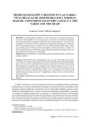
Figure 1. Schematic of an airborne laser scanning system.
Federal agencies such as the Federal Emergency Management Administration (FEMA)
and U.S. Geological Survey (USGS), along with county and state agencies, began
using LIDAR to map the terrain in flood plains and earthquake hazard zones. The Puget
Sound LIDAR Consortium, an informal group of agencies, used LIDAR in the Puget
Sound area and found previously undetected earthquake faults and large, deep-seated,
old landslides. In other parts of the country, LIDAR was used to map highly detailed
contours across large flood plains, which could be used to pinpoint areas of high risk. In
some areas, entire states have been flown with LIDAR to produce more accurate digital
terrain data for emergency planning and response. LIDAR mapping of terrain uses a
technique called “bare-earth filtering.” Laser scan data about trees and buildings are
stripped away, leaving just the bare-ground data. Fortunately for foresters and other
natural resource specialists, the data being “thrown away” by geologists provide
detailed information describing vegetation conditions and structure.
1

How Does LIDAR Work?
The use of lasers has become commonplace, from laser printers to laser surgery. In
airborne-laser-mapping, LIDAR systems are taken into the sky. Instruments are
mounted on a single- or twin-engine plane or a helicopter and data are collected over
large land areas.
Airborne LIDAR technology uses four major pieces of equipment (Figure 1). These are
a laser emitter-receiver scanning unit attached to the aircraft; global positioning system
(GPS) units on the aircraft and on the ground; an inertial measurement unit (IMU)
attached to the scanner, which measures roll, pitch, and yaw of the aircraft; and a
computer to control the system and store data. Several types of airborne LIDAR
systems have been developed; commercial systems commonly used in forestry are
discrete-return, small-footprint systems. “Small footprint” means that the laser beam
diameter at ground level is typically in the range of 6 inches to 3 feet. The laser scanner
on the aircraft sends up to 200,000 pulses of light per second to the ground and
measures how long it takes each pulse to reflect back to the unit. These times are used
to compute the distance each pulse traveled from scanner to ground. The GPS and IMU
units determine the precise location and attitude of the laser scanner as the pulses are
emitted, and an exact coordinate is calculated for each point. The laser scanner uses an
oscillating mirror or rotating prism (depending on the sensor model), so that the light
pulses sweep across a swath of landscape below the aircraft. Large areas are surveyed
with a series of parallel flight lines. The laser pulses used are safe for people and all
living things. Because the system emits its own light, flights can be done day or night,
as long as the skies are clear.
Thus, with distance and location information accurately determined, the laser pulses
yield direct, 3-D measurements of the ground surface, vegetation, roads, and buildings.
Millions of data points are recorded; so many that LIDAR creates a 3-D data cloud. After
the flight, software calculates the final data points by using the location information and
laser data. Final results are typically produced in weeks, whereas traditional groundbased
mapping methods took months or years. The first acre of a LIDAR flight is
expensive, owing to the costs of the aircraft, equipment, and personnel. But when large
areas are covered, the costs can drop to about $1 to $2 per acre. The technology is
commercially available through a number of sources.
Overview of the FUSION/LDV Analysis and Visualization
System
The FUSION/LDV software was originally developed to help researchers understand,
explore, and analyze LIDAR data. The large data sets commonly produced by LIDAR
missions could not be used in commercial GIS or image processing environments
without extensive preprocessing. Simple tasks such as extracting a sample of LIDAR
returns that corresponded to a field plot were complicated by the shear size of the data
and the variety of ASCII text formats provided by various vendors. The original versions
of the software allowed users to clip data samples and view them interactively. As a
new data set was delivered, the software was modified to read the data format and
2

features were added depending on the needs of a particular research project. After a
year or so of activity, scientists at the Pacific Northwest Research Station and the
University of Washington decided to design a more comprehensive system to support
their research efforts.
The analysis and visualization system consists of two main programs, FUSION and
LDV (LIDAR data viewer), and a collection of task-specific command line programs. The
primary interface, provided by FUSION, consists of a graphical display window and a
control window. The FUSION display presents all project data using a 2D display typical
of geographic information systems. It supports a variety of data types and formats
including shapefiles, images, digital terrain models, canopy surface models, and LIDAR
return data. LDV provides the 3D visualization environment for the examination and
measurement of spatially-explicit data subsets. Command line programs provide
specific analysis and data processing capabilities designed to make FUSION suitable
for processing large LIDAR acquisitions.
In FUSION, data layers are classified into six categories: images, raw data, points of
interest, hotspots, trees, and surface models. Images can be any geo-referenced image
but they are typically orthophotos, images developed using intensity or elevation values
from LIDAR return data, or other images that depict spatially explicit analysis results.
Raw data include LIDAR return data and simple XYZ point files. Points of interest (POI)
can be any point, line, or polygon layer that provides useful visual information or sample
point locations. Hotspots are spatially explicit markers linked to external references such
as images, web sites, or pre-sampled data subsets. Tree files contain data, usually
measured in the field, representing individual trees. Surface models, representing the
bare ground or canopy surface, must be in a gridded format. FUSION uses the PLANS
format for its surface models and provides utilities to convert a variety of formats into the
PLANS format. The current FUSION implementation limits the user to a single image,
surface model, and canopy model, however, multiple raw data, POI, tree, and hotspot
layers are allowed. The FUSION interface provides users with an easily understood
display of all project data. Users can specify display attributes for all data and can
toggle the display of the different data types.
FUSION allows users to quickly and easily select and display subsets of large LIDAR
data. Users specify the subset size, shape, and the rules used to assign colors to
individual raw data points and then select sample locations in the graphical display or by
manually entering coordinates for the points defining the sample. LDV presents the
subset for the user to examine. Subsets include not only raw data but also the portion of
the image and surface models for the area sampled. FUSION provides the following
data subset types:
• Fixed-size square,
• Fixed-size circle,
• Variable-size square,
• Variable-size circle,
• Variable-width corridor.
3

Subset locations can be “snapped” to a specific sample location, defined by POI points
to generate subsets centered on or defined by specific locations. Elevation values for
LIDAR returns can be normalized using the ground surface model prior to display in
LDV. This feature is especially useful when viewing data representing forested regions
in steep terrain as it is much easier to examine returns from vegetation and compare
trees after subtracting the ground elevation.
LDV strives to make effective use of color, lighting, glyph shape, motion, and
stereoscopic rendering to help users understand and evaluate LIDAR data. Color is
used to convey one or more attributes of the LIDAR data or attributes derived from other
data layers. For example, individual returns can be colored using values sampled from
an orthophoto of the project area to produce semi-photorealistic visual simulations. LDV
uses a variety of shading and lighting methods to enhance its renderings. LDV provides
point glyphs that range from single pixels, to simple geometric objects, to complex
superquadric objects. LDV operates in monoscopic, stereoscopic, and anaglyph display
modes. To enhance the 3D effect on monoscopic display systems, LDV provides a
simple rotation feature that moves the data subset continuously through a simple
pattern (usually circular). We have dubbed this technique “wiggle vision”, and feel it
provides a much better sense of the 3D spatial arrangement of points than provided by
a static, fixed display. To further help users understand LIDAR data, LDV can also map
orthographic images onto a horizontal plane that can be positioned vertically within the
cloud of raw data points. Bare-earth surface models are rendered as a shaded 3D
surface and can be textured-mapped using the sampled image. Canopy surface or
canopy height models are rendered as a mesh so the viewer can see the data points
under the surface.
FUSION and LDV have several features that facilitate direct measurement of LIDAR
data. FUSION provides a “plot mode” that defines a buffer around the sample area and
includes data from the buffer in a data subset. This option, available only with fixed-size
plots, makes it easy to create LIDAR data subsets that correspond to field plots. “Plot
mode” lets the user measure tree attributes for trees whose stem is within the plot area
using all returns for the tree including those outside the plot area but within the plot
buffer. The size of the plot buffer is usually set to include the crown of the largest trees
expected for a site. When in “plot mode”, FUSION includes a description of the fixedarea
portion of the subset so LDV can display the plot boundary as a wire frame
cylinder or cube and inform the user when measurement locations are within or outside
the plot boundary..
LDV provides several functions to help users place the measurement marker and make
measurements within the data cloud. The following “snap functions” are available to
help position the measurement marker:
• Set marker to the elevation of the lowest point in the current measurement area
(don’t move XY position of marker)
• Set marker to the elevation of the highest point in the current measurement area
(don’t move XY position of marker)
4

• Set marker to the elevation of the point closest to the marker (don’t move XY
position of marker)
• Move marker to the lowest point in the current measurement area
• Move marker to the highest point in the current measurement area
• Move marker to point closest to the marker
• Set marker to the elevation of the surface model (usually the ground surface)
• Change the shape and alignment of the measurement marker to better fit the
data points that represent a tree crown
The measurement marker in LDV can be elliptical or circular to compensate for tree
crowns that are not perfectly round. The measurement area can be rotated to better
align with an individual tree crown. Once an individual tree has been isolated and
measured, the points within the measurement area can be “turned off” to indicate that
they have been considered during the measurement process. This ability makes it much
easier to isolate individual trees in stands with dense canopies.
Using FUSION/LDV
To start using the FUSION system, launch FUSION and load the example project
named “demo_4800K.dvz” using the File…Open menu option. The default sample
options are set to use a stroked box. LIDAR returns will be colored according to their
height above ground.
To extract and display a sample of data, stroke a rectanglar area using the mouse. The
status display in the lower left corner of the FUSION window shows the size of the
stroked area. Try for a sample that is about 250 feet by 250 feet. This should yield a
sample of about 22,000 points. After a short time, the data subset will be displayed in
LDV. To facilitate rapid sample extraction, FUSION uses a simple indexing scheme to
organize the LIDAR data. This indexing process is necessary the first time FUSION
uses a new dataset. Subsequent samples will take less time because the data files only
need to be indexed once.
To manipulate the LIDAR data in LDV, it is easiest to imagine that the data is contained
in a glass ball. To rotate the data, use the mouse (with the left button held down) to roll
the ball and thus manipulate the data. As you move the data, LDV may display only a
subset of the points depending on the size of the sample.
Options in LDV are accessed using the right mouse button to activate a menu of
options. There are many options and the best way to understand them is to try them.
Additional functions are assigned to keystrokes. These functions are described when
you click the “About LDV” button located in the lower left corner of the LDV window.
Keyboard shortcuts are also listed on the right mouse menu.
Getting Data into FUSION
FUSION merges imagery, LIDAR data, GIS layers, field data, and surface models to
provide an intuitive interface to large project datasets. FUSION requires an ortho-
5

ectified image for the project area (image can be created in FUSION using LIDAR
return data) and LIDAR data. Other data types are optional.
FUSION currently reads several ASCII file formats and LAS files. Its native format,
called LDA, is an indexed binary format that allows rapid random access to large
datasets. FUSION also reads LAS files and uses the same indexing scheme to facilitate
rapid data sampling. LAS files do not need to be converted to the LDA format for use inf
FUSION. Utilities are included that convert ASCII files into the native binary format.
FUSION requires an ortho-rectified image and an associated world file to provide
scaling information and a backdrop for the project. A utility is included to create an
image using the intensity value or the elevation recorded with each LIDAR return.
FUSION reads surface models (ground, canopy, or other surfaces of interest) stored in
the PLANS DTM format (described in Appendix A: File Formats). FUSION provides
conversion tools to convert surface models stored in other formats into the PLANS
format. Supported formats include USGS ASCII DEM, USGS SDTS, SURFER, and
ASCII grid.
Converting LIDAR Data Files into LDA Files
FUSION provides a two conversion utilities that convert ASCII data formats into the LDA
format. The utilities are accessed using the “Utilities” button on the FUSION control
panel. The “Import LIDAR data in specific ASCII formats…” button brings up the dialog
for converting ASCII data files stored in specific formats. The formats include a generic
XYZ point format but, for the most part, are specific to data that were acquired while
FUSION was being developed. ASCII input files typically have the .XYZ extension
(using this extension will make it easier to select the files). The formats supported are
described elsewhere in this document. The “Import generic ASCII LIDAR data…” option
allows the user to define the format of the ASCII data and specify the LIDAR fields that
will be converted. FUSION’s internal LDA format includes the following attributes for
each LIDAR return: pulse number, return number, X, Y, Elevation, scan/nadir angle, and
intensity. For datasets that do not include all attributes, you can specify default values
for the missing attributes.
LAS format files are read and used directly by FUSION. The same indexing scheme is
used to facilitate rapid file access but the files are not converted to the LDA format. The
first time a sample is extracted from a LAS file, the index files are created. Subsequent
sampling operations use the newly created index files.
Creating Images Using LIDAR Data
FUSION provides a utility that uses the intensity value or the elevation for each LIDAR
return to construct an orthographic image and the associated world file to provide
georeferencing information. This utility is accessed using the “Tools” menu and the
“Create an image using LIDAR point data…” option under “Miscellaneous utilities”. The
image can be built using several LDA or LAS formatted files (in case the project
organizes data into multiple files). For most data, you will want to clamp the intensity
6

ange to a specific set of values. To help determine appropriate values for the color
mapping, the “Scan for data ranges” button can be used to report the range of values in
the LDA file and a display a histogram of the intensity values. In most cases, you should
not map the full range of intensity values to the grayscale image. Our experience with
several vendors has taught us that most vendors don’t know much about the intensity
values and can’t even tell you the correct range of values recorded in their data. You
can change the pixel size for the image but the default of 1 unit (same planimetric units
in LIDAR data) generally provides a reasonable image. For low density datasets (

within the sample area even when you know for sure that you are sampling within the
data coverage area.
8

Keyboard Commands for FUSION
The following keystroke and mouse commands area available in FUSION after an
image has been loaded.
Keystroke/mouse Description
action
Middle mouse Pan the display to the location of the mouse cursor
button
Left mouse button Begin a sample using the location of the mouse cursor
Right mouse
button
Cancel a sample (the right mouse button must be pressed while
the left button is pressed)
Mouse wheel Scroll the display up and down
up/down
Shift & mouse Scroll the display left and right
wheel up/down
Ctrl & mouse Zoom the display in and out
wheel up/down
Left arrow
Pan display to the right
Right arrow Pan display to the left
Up arrow
Pan display down
Down arrow Pan display up
(+) plus key Zoom in
(-) minus key Zoom out
Home
Zoom to image extent
F5
Redraw the display
9

Keyboard Commands for LDV
The following keystroke and mouse commands are available in LDV. Many of these
commands can also be accessed using the right-mouse menu.
Keystroke/mouse
action
Up arrow
8 on numeric
keypad
Down arrow
2 on numeric
keypad
Right arrow
6 on numeric
keypad
Left arrow
4 on numeric
keypad
Page up
9 on numeric
keypad
Page down
3 on numeric
keypad
Home
5 on numeric
keypad
7 on numeric
keypad
Shift & left arrow
Control & left
arrow
Shift & control &
left arrow
Shift & right arrow
Control & right
arrow
Shift & control &
right arrow
Shift & up arrow
Context
Viewing
Viewing
Viewing
Viewing
Viewing
Viewing
Viewing
Measurement
marker on
Measurement
marker on
Measurement
marker on
Measurement
marker on
Measurement
marker on
Measurement
marker on
Measurement
marker on
Description
Rotate around screen X axis (away from
viewer)
Rotate around screen X axis (toward viewer)
Rotate around screen Y axis (away from
viewer)
Rotate around screen Y axis (toward viewer)
Rotate around screen Z axis (counterclockwise)
Rotate around screen Z axis (clockwise)
Reset rotation to original state
Move marker in negative direction along the
X axis of the data (not X axis of screen)
Rotate marker 1 degree in positive direction
Rotate marker 10 degrees in positive
direction
Move marker in positive direction along the X
axis of the data (not X axis of screen)
Rotate marker 1 degree in negative direction
Rotate marker 10 degrees in negative
direction
Move marker in positive direction along the Y
axis of the data (not Y axis of screen)
10

Keystroke/mouse Context
Description
action
Control & up arrow Measurement
marker on
Increase long axis of marker making the
marker more elliptical (small step)
Shift & control &
up arrow
Measurement
marker on
Increase long axis of marker making the
marker more elliptical (large step)
Shift & down arrow Measurement
marker on
Move marker in negative direction along the
Y axis of the data (not Y axis of screen)
Control & down
arrow
Measurement
marker on
Decrease long axis of marker making the
marker more elliptical (small step)
Shift & control &
down arrow
Measurement
marker on
Decrease long axis of marker making the
marker more elliptical (large step)
Escape
Wiggle-vision on
Scan-vision on
Measurement
Stop motion or stop scanning of clipping
planes
Clear marks and measurement points
marker on
Backspace Measurement Deletes last measurement point
marker on with
measurement line
Enter
Measurement Save measurement point
marker on
Space Viewing Activate right-mouse-button menu
+ (plus key) Viewing with Increase transparency of the image plate
image plate active
+ (plus key) Viewing with Increase transparency of the surface model
surface active
Control & + (plus Viewing using Increase size of point markers
key)
fixed size markers
- (minus key) Viewing with Decrease transparency of the image plate
image plate active
- (minus key) Viewing with Decrease transparency of the surface model
surface active
Control & - (minus Viewing using Decrease size of point markers
key)
fixed size markers
Letter A
Measurement
marker on
Turn on display of points within
measurement area and above current
marker height
Shift & letter A Viewing Turn on display of all data points
Letter B
Measurement
marker on
Letter C
Measurement
marker on
Turn on display of points within
measurement area and below current marker
height
Move marker to the height of the closest
point within the measurement area
11

Keystroke/mouse
action
Shift & letter C
Letter F
Letter G
Letter H
Shift & letter H
Letter I
Shift & letter I
Control & letter I
Shift & letter I
Letter L
Shift & letter L
Letter O
Letter R
Letter S
Letter T
Letter X
Context
Measurement
marker on
Measurement
marker on
Measurement
marker on and
surface display
enabled
Measurement
marker on
Measurement
marker on
Image plate
enabled
Image plate
enabled
Image plate
enabled
Image plate
enabled
Measurement
marker on
Measurement
marker on
Measurement
marker on
Measurement
marker on
Measurement
marker on
Measurement
marker on
YZ clipping
enabled
Description
Center the measurement area on the closest
point and move the marker to the height of
the closest point within the measurement
area
Fits the measurement marker to the data
points above the measurement plate. Use
this option to rotate and adjust the
dimensions of the marker to better “fit” the
marker to a tree crown.
Move measurement marker to ground
elevation
Move marker to the height of the highest
point within the measurement area
Center the measurement area on the highest
point and move the marker to the height of
the highest point within the measurement
area
Lower image plate (small step)
Raise image plate (small step)
Lower image plate (large step)
Raise image plate (large step)
Move marker to the height of the lowest point
within the measurement area
Center the measurement area on the lowest
point and move the marker to the height of
the lowest point within the measurement
area
Reset measurement marker to a circle
Turn off display of points within
measurement area
Move measurement area to the current
marked point (indicated with a 3D “+”)
Toggle display of points within measurement
area
Lower clipping plane (small step)
12

Keystroke/mouse Context
Description
action
Shift & letter X YZ clipping Raise clipping plane (small step)
enabled
Control & letter X YZ clipping Lower clipping plane (large step)
enabled
Shift & letter X YZ clipping Raise clipping plane (large step)
enabled
Letter Y
XZ clipping Lower clipping plane (small step)
enabled
Shift & letter Y XZ clipping Raise clipping plane (small step)
enabled
Control & letter Y XZ clipping Lower clipping plane (large step)
enabled
Shift & letter Y XZ clipping Raise clipping plane (large step)
enabled
Letter Z
XY clipping Lower clipping plane (small step)
enabled
Shift & letter Z XY clipping Raise clipping plane (small step)
enabled
Control & letter Z XY clipping Lower clipping plane (large step)
enabled
Shift & letter Z XY clipping Raise clipping plane (large step)
enabled
F3 Viewing Open ground augmentation point dialog
F4 Viewing Open bare ground model dialog*
F5 Viewing Open segmentation dialog*
F7 Viewing Open plot location dialog*
F8 Viewing Open attribute clipping dialog
F9 Viewing Open tree measurement dialog
*These features are considered experimental and not available in publicly released
versions of FUSION/LDV.
13

Command Line Utility and Processing Programs
Command line utilities and processing programs, called the FUSION LIDAR Toolkit or
FUSION-LTK, provide extensive processing capabilities including bare-earth point
filtering, surface fitting, data conversion, and quality assessment for large LIDAR
acquisitions. These programs are designed to run from a command prompt or using
batch programs. The FUSION-LTK Programs generally have required and optional
parameters as well as switches to control program options. Switches should be
preceded by a forward slash “/”. If a switch has multiple parameters after the colon “:”,
they should be separated by a single comma “,” with no spaces before or after the
comma. Command line programs display their syntax when executed with no
parameters.
Command Line Options Shared By All Programs
There are several switches common to all FUSION-LTK programs. They control use of
the FUSION-LTK master logfile, activate interactive run modes (when available), and
report program version information. The switches common to all FUSION-LTK programs
are:
interactive
quiet
verbose
newlog
log:name
version
Present a dialog-based interface. The /interactive switch is not
supported in most programs.
Suppresses the display of all status information during the run.
Displays status information as a program runs. The information may
describe the analysis progress or simply provide an indication that
the program is still running. The additional information displayed
when using the /verbose switch is not written to the LTKCL log file.
Erase the existing LTKCL_master.log file and start a new log file.
Use the name specified for the log file.
Displays only version information for the program.
Command Log Files
All FUSION-LTK programs write entries into the FUSION-LTK master log files. Normally
these files are stored in the directory containing the FUSION programs in files named
LTKCL_master.log and LTKCL_master.csv. The /log:name switch can be used to force
a program to write its log entries to a different file. The environment variable, LTKLOG,
can also be used to change the default log file. When using LTKLOG, set the variable to
the full path for the log file (include the folder) unless you want the log file created in the
current directory. The .csv log name will be created from the LTKLOG variable using
and extension of .csv. The LTKLOG environment variable can be set from a command
prompt using the following DOS command:
set LTKLOG=mylogfile.log
Once the variable is set, it will be available for all programs run in the same DOS
window (command prompt window). Other windows will not be able to “see” the
variable. The variable can be cleared using the following DOS command:
set LTKLOG=
14

Use of the LTKLOG environment variable is most effective when the variable is set at
the beginning of a batch program used to accomplish some processing task and cleared
at the end of the program. In this way you can direct all log entries associated with a
project to the same log files.
The .log entries include all output normally displayed on the screen when one of the
FUSION-LTK programs runs. All command line parameters are reported and any output
files are listed along with their creation date and time. Output related to the use of the
/verbose switch is not included in the log file. The .csv entries simply list the command
lines used to invoke various FUSION-LTK programs. The following columns are
included in the .csv log:
Program name
Version
Program build date
Command line parameters
Start time
Stop time
Elapsed time (seconds)
Status indicator
The logs have proven very useful when trying to remember the command line options
used to create a specific output product or the program version used to conduct an
analysis. By matching the file name, date and time to a log entry, you can easily repeat
a processing task. The log file can become quite large over time so it is important to
either manage the log by archiving the file and then deleting it (a new log file will be
started the next time FUSION-LTK program is used) or by using specific log files for
different projects. The latter option is facilitated by the /log:name switch but this switch
must be used for all programs that are to write to the specified log file. Using the
LTKLOG (see Appendix B: DOS Batch Programming and the FUSION LIDAR Toolkit for
details) environment variable allows you to change the log file without specifying the log
on each program command line.
FUSION-LTK Overview
The command line utility and processing programs are grouped into six types:
Point
Surface
Image
Conversion
Info
Misc
Operates on point data.
Operates on surfaces.
Operates on images.
Converts data from one format to another.
Provides descriptive information for a data source.
Miscellaneous utilites.
In general, Point utilities use point cloud data to produce either new point clouds or
surfaces and Surface utilities use surfaces to produce new surfaces or point data.
Version 2.61 of FUSION does not include any Surface utilities. However, there are
15

several Surface utilities under development that will be included in a future version. The
set of programs included in the toolkit has, and will continue to, evolve as new analysis
methods are discovered or developed. The current set of programs addresses most
tasks commonly needed when LIDAR data are obtained for a forestry-related project.
The following table summarizes the toolkit programs:
Program name Category Description
ASCII2DTM Conversion Converts an ASCII raster surface model into
the PLANS format used by FUSION
ASCIIImport Conversion Converts variable format ASCII LIDAR data to
LDA or LAS format
CanopyModel Point Creates a canopy surface model from a point
cloud
Catalog Point Prepares a report describing a LIDAR dataset
and optionally indexes all data files for use in
FUSION
ClipData Point Clips subsamples of data using the lower left
and upper right corners of the area
ClipDTM Surface Clips a portion of a DTM using a userspecified
extent.
CloudMetrics Point Computes metrics for a LIDAR data set
(usually a data sample)
Cover Point Computes cover estimates using a bare-earth
surface model and point cloud
CSV2Grid Conversion Converts data stored in commas separated
value (CSV) format into PLANS dtm format
DensityMetrics Point Computes point density metrics using
elevation-based slices
DTM2ASCII Conversion Converts PLANS dtm files into ASCII raster
format
DTM2ENVI Conversion Converts PLANS dtm files into ENVI standard
format files with associated header files
DTM2TIF Conversion Converts PLANS dtm files into TIF grayscale
images
DTM2XYZ Conversion Converts PLANS dtm files into XYZ points
DTMDescribe Misc Outputs information from PLANS dtm file
headers to CSV file
DTMHeader Info Display header information for PLANS format
surface models and edit some header
elements
FirstLastReturn Point Extracts first and last returns from a point
cloud
GridMetrics Point Computes metrics for points falling within
each grid cell
GridSample Surface Extracts samples of grid values around an XY
position
16

GridSurfaceCreate Point Creates a gridded surface model from point
data
GroundFilter Point Filters a point cloud to identify bare-earth
points
ImageCreate Point Creates an image from LIDAR data files using
the intensity values and specified color ramp
IntensityImage Point Creates images using the intensity values
from a point cloud
LDA2ASCII Conversion Converts point data stored in LDA format to
ASCII text format
LDA2LAS Conversion Converts LDA point cloud files to LAS format
(not all fields in LAS format are populated)
MergeData Point Merges serveral point cloud files into a single
file
MergeDTM Surface Merges several DTM files into a single DTM
file
PolyClipData Point Clips point data using polygons stored in
shapefiles
SurfaceSample Surface Interpolates surface values for XY positions
TiledImageMap Image Creates HTML web page linking a master
image to individual image tiles using an HTML
image map
TINSurfaceCreate Point Creates a surface model using all points in
LIDAR data files (uses TIN then grids to final
cell size)
UpdateIndexChecksum Misc Updates the checksum used with a data index
file (used to prevent reindexing after FUSION
upgrade, post spring 2006)
ViewPic Image Displays image files stored in a variety of
formats
XYZ2DTM Conversion Creates a PLANS dtm file from XYZ grid
points
XYZConvert Conversion Converts ASCII data files into LDA format and
indexs the LDA files
The following sections describe the LTK programs in detail. These descriptions include
a brief overview of each program, detailed syntax information and command line
parameter descriptions, a technical description of the algorithms involved, and
examples showing common uses for the program. For programs that implement
algorithms developed by other researchers, appropriate citations are included.
17

ASCII2DTM
Overview
ASCII2DTM converts raster data stored in ESRI ASCII raster format into a PLANS
format data file. Data in the input ASCII raster file can represent a surface or raster
data. ASCII2DTM converts areas containing NODATA values into areas with negative
elevation values in the output data file.
Syntax
ASCII2DTM [switches] surfacefile xyunits zunits coordsys zone horizdatum vertdatum
gridfile
surfacefile Name for output canopy surface file (stored in PLANS DTM format
with .dtm extension).
xyunits Units for LIDAR data XY:
M for meters,
F for feet.
zunits Units for LIDAR data elevations:
M for meters,
F for feet.
coordsys Coordinate system for the canopy model:
0 for unknown,
1 for UTM,
2 for state plane.
zone
horizdatum
vertdatum
Gridfile
Coordinate system zone for the canopy model (0 for unknown).
Horizontal datum for the canopy model:
0 for unknown,
1 for NAD27,
2 for NAD83.
Vertical datum for the canopy model:
0 for unknown,
1 for NGVD29,
2 for NAVD88,
3 for GRS80.
Name of the ESRI ASCII raster file containing surface data.
Switches
The standard FUSION-LTK toolkit switches are supported,
Technical Details
ASCII2DTM recognizes both the (xllcorner, yllcorner) and (xllcenter, yllcenter) methods
for specifying the location of the raster data. The PLANS DTM format always assumes
that the data point (grid point) in the lower left corner is the model origin and adjusts the
location of the raster data accordingly.
18

Examples
The following command converts the ASCII raster file named canopy_southern.asc into
a PLANS format data file named canopy.dtm. Data use the UTM projection in zone 10,
NAD83, NAVD88, and meters for both planimetric and elevation values.
ASCII2DTM canopy_southern.asc m m 1 10 2 2 canopy.dtm
19

ASCIIImport
Overview
ASCIIImport allows you to use the configuration files that describe the format of ASCII
data files to convert data into FUSION’s LDA format. The configuration files are created
using FUSION’s Tools…Data conversion…Import generic ASCII LIDAR data… menu
option. This option allows you to interactively develop the format specifications needed
to convert and ASCII data file into LDA format.
Syntax
ASCIIImport [switches] ParamFile InputFile [OutputFile]
ParamFile Name of the format definition parameter file (created in FUSION's
Tools...Data conversion...Import generic ASCII LIDAR data... menu
option.
InputFile Name of the ASCII input file containing LIDAR data.
OutputFile Name for the output LDA or LAS file (extension will be provided
depending on the format produced). If OutputFile is omitted, the
output file is named using the name of the input file and the
extension appropriate for the format (.lda for LDA, .las for LAS).
Switches
LAS
The standard FUSION-LTK toolkit switches are supported. Progress
information for the conversion is displayed when the /verbose switch
is used.
Output file is stored in LAS version 1.0 format.
Technical Details
ASCIIImport allows FUSION to read most ASCII LIDAR data and convert it to the LDA
format. In operation, each line of the data file is read and parsed according the format
specifications. In general, one point record is created for each line in the input file. The
format specifications allow you to specify a variety of characters that separate data
values and assign specific columns of the data to LIDAR returns variables. ASCII files
with descriptive headers can be processed by specifying the number of lines to skip at
the beginning of the file.
Examples
The following command line converts the ASCII data file named tile0023.txt into an LDA
file named tile0023.lda using the format specifications stored in the parameter file
named project.importparam:
ASCIIImport project.importparam tile0023.txt
The following command line provides progress feedback while converting the ASCII
data file named tile0023.txt into an LDA file named 0023.lda using the format
specifications stored in the parameter file named project.importparam:
ASCIIImport /verbose project.importparam tile0023.txt 23.lda
20

CanopyModel
Overview
CanopyModel creates a canopy surface model using a LIDAR point cloud. By default,
the algorithm used by CanopyModel assigns the elevation of the highest return within
each grid cell to the grid cell center. CanopyModel provides for smoothing of the
generated surface using a median or a mean filter or both. Specialized logic, activated
using the /peaks switch, preserves local maxima in the surface while smoothing to force
the surface to adhere to the tops of trees. CanopyModel provides options to compute a
texture metric (coefficient of variation of surface values within an n by n window), slope,
or aspect for the canopy model and output them as the final surface. When used with a
bare-earth model, CanopyModel subtracts the ground elevations from the return
elevations to produce a canopy height model. Output from CanopyModel is a PLANS
format DTM file that uses floating point elevation values and contains coordinate
projection information.
Syntax
CanopyModel [switches] surfacefile cellsize xyunits zunits coordsys zone horizdatum
vertdatum datafile1 datafile2 …
surfacefile
cellsize
xyunits
zunits
coordsys
zone
horizdatum
vertdatum
datafile1
Name for output canopy surface file (stored in PLANS DTM format
with .dtm extension).
Desired grid cell size in the same units as LIDAR data.
Units for LIDAR data XY:
M for meters,
F for feet.
Units for LIDAR data elevations:
M for meters,
F for feet.
Coordinate system for the canopy model:
0 for unknown,
1 for UTM,
2 for state plane.
Coordinate system zone for the canopy model (0 for unknown).
Horizontal datum for the canopy model:
0 for unknown,
1 for NAD27,
2 for NAD83.
Vertical datum for the canopy model:
0 for unknown,
1 for NGVD29,
2 for NAVD88,
3 for GRS80.
First LIDAR data file (LDA, LAS, ASCII LIDARDAT formats)...may
be wildcard or name of text file listing the data files. If wildcard or
text file is used, no other datafile# parameters will be recognized.
22

datafile2
Second LIDAR data file (LDA, LAS, ASCII LIDARDAT formats).
Several data files can be specified. The limit depends on the length
of each file name. When using multiple data files, it is best to use a
wildcard for datafile1 or create a text file containing a list of the data
files and specifying the list file as datafile1.
Switches
median:#
smooth:#
texture:#
slope
aspect
outlier:low,high
ground:file
peaks
Apply median filter to model using # by # neighbor window.
Apply mean filter to model using # by # neighbor window.
Calculate the surface texture metric using # by # neighbor window.
Calculate surface slope for the final surface.
Calculate surface aspect for the final surface.
Omit points with elevations below low and above high if used with a
bare-earth surface this option will omit points with heights below low
or above high.
Use the specified bare-earth surface model to normalize the LIDAR
data.
Preserve localized peaks in the final surface. Only useful with
/median or /smooth.
The order of the filter median and smooth switches is important. The first filter specified
on the command line will be the first filter applied to the model (median or smooth). You
cannot use /texture:#, /slope, and /aspect in combination.
Technical Details
CanopyModel uses the return with the highest elevation to compute the canopy surface
model. If the /ground switch is used to produce a canopy height model, the ground
elevation interpolated from the bare-earth surface model is subtracted from the return
elevation prior to determining the highest return value. It is important that the bare-earth
model truly represents the ground surface as any spikes due to residual vegetation
returns in the point set used to create the bare-earth model will result in incorrect return
heights and possible an incorrect canopy height model.
The behavior of the /outlier switch depends on whether of not the /ground switch is
used. Without the /ground switch, /outlier uses the return elevations and the low and
high values to filter out returns based on the elevation. When used with the /ground
switch, the height above ground is used to filter out returns. In general, the /outlier
switch is more useful when used with the /ground switch.
When either of the smoothing switches is used (/smooth or /median), an initial surface is
computed using the highest return elevation for each cell. Then the initial surface is
used to produce the final, smoothed surface. During the smoothing operation, the
/peaks switch activates logic that compares the cell being modified to the other cells in
the smoothing window. If the target cell elevation is higher that all the neighboring cell
elevations, its elevation will not be changed.
23

CanopyModel can be used with bare-earth point sets to create a ground surface model
that sits on top of the bare-earth points. In contrast, GridSurfaceCreate creates a
surface that represents the average elevation for all points within a cell so the final
surface it produces lies within the bare-earth point set. The /texture, /slope, and /aspect
switches can be used with bare-earth point sets to produce descriptive layers for the
ground surface.
Examples
The following command will create a canopy surface model using a 5- by 5-meter grid.
XY and elevation data are in meters. Data are referenced in the UTM coordinate system
in zone 10. The horizontal datum is NAD83 and the vertical datum is NAVD88. Data
files used to create the surface are listed in a text file named list.txt (shown below).
CanopyModel canopy_surface.dtm 5 m m 1 10 2 2 list.txt
The text file used to specify data file names contains the following:
000263.las
000264.las
000265.las
The following command will create the same canopy surface model but in this example,
data files are listed explicitly on the command line.
CanopyModel canopy_surface.dtm 5 m m 1 10 2 2 000263.las 000264.las 000265.las
The following command will create the same canopy surface model but in this example,
a wildcard specifier is used to reference the data files. When using wildcard specifiers,
you need to make sure the specifier will result in the correct list of data files. You can
test this by using the DIR command along with the specifier to verify the files that will be
used to create the surface model (e.g., DIR *.las)
CanopyModel canopy_surface.dtm 5 m m 1 10 2 2 *.las
The following command will create the surface model and then apply a 5 by 5 cell
median filter to smooth the surface (/median:5). Local maxima will be preserved in the
surface (/peaks) to force the surface to adhere to the tops of trees.
CanopyModel /peaks /median:5 canopy_surface.dtm 5 m m 1 10 2 2 *.las
24

Catalog
Overview
Catalog produces a set of descriptive reports describing several important
characteristics of LIDAR data sets. It is most often used to evaluate a new acquisition
for internal quality, completeness of data coverage and return or pulse density. The
primary output of Catalog is a web page that contains a summary of all data tiles
evaluated including attribute summaries for each tile and overall summaries for the
entire data set. Catalog provides options that will create the index files needed to use
the LIDAR data with FUSION making it the logical first step in any analysis procedure.
In addition to the web page, Catalog can produce images representing the coverage
area, pulse and return densities, and intensity values for the entire acquisition. All
images produced by Catalog have associated world files so they can be used within
FUSION to provide a frame-of-reference for analysis. Catalog also produces a FUSION
hotspot file that provides specific details for each data tile in the FUSION environment.
Syntax
Catalog [switches] datafile [catalogfile]
datafile
catalogfile
Switches
image
index
newindex
drawtiles
coverage
density:cell,min,max
firstdensity:cell,min,max
LIDAR data file template or name of a text file containing a
list of file names (list file must have .txt extension).
Base name for the output catalog file (extensions will be
added).
Create image files showing the coverage area for each
LIDAR file.
Create LIDAR data file indexes if they don't already exist.
Create new LIDAR data file indexes for all files (even if
they already exist).
Draw data file extents and names on the intensity image.
Create one image that shows the nominal coverage area
for all data files included in the catalog. Also creates a
FUSION hotspot file that provides details for each file in the
catalog.
Creates an image for all data files that shows the return
density for the area represented by each pixel. cell is the
pixel area, min is the minimum acceptable point density per
unit area, and max is the upper limit for the acceptable
density range. Cells with point densities falling within the
min-max range are colored green, cells with point densities
below the minimum are colored red, and cells with
densities above the maximum are colored blue.
Creates an image for all data files that shows the density of
first returns for the area represented by each pixel. cell is
the pixel area, min is the minimum acceptable point density
25

intensity:cell,min,max
bmp
outlier:multiplier
per unit area, and max is the upper limit for the acceptable
density range. Cells with first return densities falling within
the min-max range are colored green, cells with point
densities below the minimum are colored red, and cells
with densities above the maximum are colored blue.
Creates an intensity image for all data files using the
average intensity for all first returns within each pixel. cell is
the pixel area, min is the minimum intensity value, and max
is the maximum intensity value. A black to white color ramp
is mapped to the range of intensity values defined by min
and max. Ideally, min and max correspond to the range of
intensity values present in the data. However, you may not
always know the range of values for a given data set.
Save second copy of intensity image in BMP format with
associated world file.
Performs a simple analysis to identify data tiles that might
contain elevation outliers. The analysis marks tiles where
the minimum, maximum, or range of elevations are outside
the range defined by:
mean value +- multiplier * std dev
The default multiplier is 2.0.
The "image" switch requires data file indexes. If indices do not already exist for all data
files, use the "index" option to force their creation.
Technical Details
When creating intensity images, Catalog uses the average intensity for all returns within
a cell to compute the grayscale color for the cell. This logic differs from that of the
CreateImage program which uses the maximum intensity value for a cell. As a result,
the images created by Catalog will differ from those created by CreateImage.
The outlier detection logic in Catalog is very limited. In areas dominated by flat or
relatively flat topography, the logic will usually identify data tiles with erroneous returns
due to birds, multipathing, or system noise. In areas with steep topography, the logic will
often miss such artifacts since the erroneous returns have elevations that may be
outside the range in the vicinity of the return but are within the range for the entire data
tile.
The /density and /firstdensity switches should not be used with very small cell sizes
(area

scan will be highly variable (for zig-zag scan patterns) when evaluated using a small cell
size.
The /image switch is obsolete. Use the /intensity switch instead. /image produces one
image for each data tile and while this may be useful for small data sets containing only
a few tiles, it produces a large number of images that must be examined when the data
set is large with many tiles. In addition, /image requires data indexing prior to creation of
the images. /intensity does not require index files and may be much faster when index
files are not needed for other analysis tasks.
Examples
The following command produce a simple summary report containing the coordinate
extents, total number of returns, and the nominal return density for each data tile.
Output includes a web page (HTML file) and a spreadsheet compatible file containing
the summary information. No image files are produced.
Catalog *.las
The following command produces the overall summary information, creates index file for
FUSION, and produces intensity images and images depicting the pulse and return
densities. The intensity image uses a 2.5- by 2.5-meter pixel (area = 6.25 m 2 ) and maps
the range of intensity values from 0 to 90 to a grayscale color ramp. The return density
image uses a 5- by 5-meter pixel (area = 25 m 2 ) and colors areas with less the 2
returns/m 2 red, cells with 2 to 8 returns/m 2 green and cells with more than 8 returns/m 2
blue. The first return (or pulse) density image uses a 5- by 5-meter pixel (area = 25 m 2 )
and colors areas with less the 1 pulse/m 2 red, cells with 1 to 6 pulses/m 2 green and cells
with more than 6 pulses/m 2 blue.
Catalog /index /intensity:6.25,0,90 /density:25,2,8 /firstdensity:25,1,6 *.las
27

ClipData
Overview
ClipData creates sub-samples of LIDAR data for various analysis tasks. The subsample
can be round or rectangular and can be large or small. ClipData provides many
of the same sampling options found in FUSION but it is not used by FUSION to perform
subsampling of LIDAR data sets (FUSION has its own logic to accomplish this task).
ClipData is often used to create sample of LIDAR returns around a specific point of
interest such as a plot center or GPS measurement point. Subsequent analyses using
programs like CloudMetrics facilitate comparing field data to LIDAR point cloud metrics.
ClipData can also sub-sample data within the sample area using the elevation values
for the returns. When used in conjunction with a bare-earth surface model, this logic
allows for sampling a range of heights above ground within the sample area.
ClipData can extract specific returns (1 st , 2 nd , etc) or first and last returns (LAS files only)
for the sample area. This capability, when used with a large sample area, can extract
specific returns from an entire data file.
As part of the sampling process, ClipData can add (or subtract) a fixed elevation from
each return elevation effecting adjusting the entire sample up or down. This capability,
when used with a large sample area, can adjust entire data files up or down to help
align data from different LIDAR acquisitions.
Syntax
ClipData [switches] InputSpecifier SampleFile MinX MinY MaxX MaxY
InputSpecifier
SampleFile
MinX MinY
MaxX MaxY
LIDAR data file template, name of a text file containing a list of file
names (must have .txt extension), or a FUSION Catalog CSV file.
Name for subsample file (.lda extension will be added).
Lower left corner of the sample area bounding box.
Upper right corner of the sample area bounding box.
Switches
shape:#
Shape of the sample area:
0 rectangle,
1 circle.
decimate:# Skip # points between included points (must be > 0).
dtm:file
zmin:#
zmax:#
Use the specified bare-earth surface model to normalize the LIDAR
data (subtract the bare-earth surface elevation from each lidar point
elevation). Use with /zmin to include points above zmin or with /zmax
to include points below zmax (file must be FUSION/PLANS format).
Include points above # elevation. Use with /dtm to include points
above # height.
Include points below # elevation. Use with /dtm to include points
below # height.
28

zpercent:# Include only the upper # percent of the points. If # is (-) only the
lower # percent of the points. # can be -100 to +100.
height Convert point elevations into heights above ground using the
specified DTM file. Always Used with /dtm.
zero
Save subsample files that contain no data points. This is useful when
automating conversion and analysis tasks and expecting a
subsample file every time ClipData is executed.
biaselev:# Add an elevation offset to every LIDAR point: # can be + or -.
return:string Specifies the returns to be included in the sample. String can include
A,1,2,3,4,5,6,7,8,9,F,L. A includes all returns. For LAS files only: F
indicates first of many returns, L indicates last of many returns. F
and L will not work with non-LAS files.
noindex Do not use the data index files to access the data. This is useful
when the order of the data points is important or when all returns for
a single pulse need to stay together in the subsample file.
Index
Create FUSION index files for the SampleFile.
Technical Details
ClipData uses FUSION index files, when they are available, to determine which data
files need to be read to find returns within the sample area and to help reduce the
number of points that need to be read within a given data file. Performance will be
significantly slower if the data has not been indexed. Indexing is best accomplished
using the Catalog program.
If the /noindex switch is used, the index files will not be used. This is most often used
when you need to preserve the original pulse and point order after the clipping process.
When you specify the /index switch, ClipData creates FUSION index files for the sample
file if it contains points. Having the index file significantly improves the performance of
several LTK programs.
The method used to compute the radius for round sample uses the average of the width
and height of the sample area. This means that you should use sample corner
coordinates that define a square area. Anything other than a square area will yield
unexpected results when used with the /shape:1 switch.
Examples
The following command clips a 100- by 100-meter square sample from a single data file
(000263.las) and stores it in a file names test.lda:
clipdata 000263.las test 520500 5196000 520600 5196100
The following command clips a 100- by 100-meter round sample from a single data file
(000263.las) and stores it in a file names test.lda:
clipdata /shape:1 000263.las test 520500 5196000 520600 5196100
29

ClipDTM
Overview
ClipDTM clips a portion of the gridded surface model and stores it in a new file. The
extent of the clipped model is specified using the lower left and upper right corner
coordinates.
Syntax
ClipDTM [switches] InputDTM OutputDTM MinX MinY MaxX MaxY
InputDTM
OutputDTM
MinX MinY
MaxX MaxY
Switches
Name of the existing PLANS format DTM file to be clipped.
Name for the new PLANS format DTM file.
Lower left corner for the output DTM.
Upper right corner for the output DTM.
The standard FUSION-LTK toolkit switches are supported.
Technical Details
When clipping a DTM, the lower left corner will be rounded down and the upper right
corner will be rounded up to the nearest multiple of the InputDTM cell size. If the
specified extent is outside the DTM area, the extent will be adjusted to match the extent
of the InputDTM. The OutputDTM will use the same cell size and projection information
as the InputDTM.
Examples
The following command line clips a subsample of the surface stored in FL_allarea.dtm
and stores the resulting surface in clip.dtm:
ClipDTM FL_allarea.dtm clip.dtm 567320.4 7654984.2 569490.6 7655439.9
30

CloudMetrics
Overview
CloudMetrics computes a variety of statistical parameters describing a LIDAR data set.
Metrics are computed using point elevations and intensity values (when available). In
operation, CloudMetrics produces one record of output for each data file processed.
Input can be a single LIDAR data file, a file template that uses DOS file specifier rules, a
simple text file containing a list of LIDAR data file names, or a LIDAR data catalog
produced by the Catalog utility. Output is appended to the specified output file unless
the /new switch is used to force the creation of a new output data file. Output is
formatted as a comma separated value (CSV) file that can be easily read by database,
statistical, and MS-Excel programs.
CloudMetrics is most often used with the output from the ClipData program to compute
metrics that will be used for regression analysis in the case of plot-based LIDAR
samples or for tree classification in the case of individual tree LIDAR samples.
Syntax
CloudMetrics [switches] InputDataSpecifier OutputFileName
InputDataSpecifier
OutputFileName
Switches
above:#
new
firstinpulse
highpoint
id
htmin:#
LIDAR data file template, name of text file containing a list of
LIDAR data file names (must have .txt extension), or a catalog
file produced by the Catalog utility.
Name for output file to contain cloud metrics (using a .csv will
associate the files with MS-Excel).
Compute the proportion of first returns above the specified
heightbreak. This metric serves as a canopy cover estimate
when the LIDAR data covers forested areas. This option is
usually used when the LIDAR point data has been normalized
using a ground surface model.
Creates a new output file and deletes any existing file with the
same name. A header is written to the new output file.
Use only the first return for a pulse to compute metrics. Such
returns may not always be labeled as return 1.
Produce a limited set of metrics that includes only the highest
return within the data file.
Parse the data file name to create an identifier for the output
record. Data file names should include a number (e.g.
sample003.lda) or the default identifier of 0 will be assigned to
the file. The identifier is placed in the first column of the output
record before the input file name.
Use only returns above # (use when data in the input data files
have been normalized using a ground surface model.
31

Technical Details
CloudMetrics computes the following statistics using elevation and intensity values for
each LIDAR sample:
Total number of returns
Minimum
Maximum
Mean
Median
Mode
Standard deviation
Variance
Interquartile distance
Skewness
Kurtosis
AAD (Average Absolute Deviation)
Percentile values (5 th , 10 th , 20 th , 25 th , 30 th , 40 th , 50 th , 60 th , 70 th , 75 th , 80 th , 90 th ,
95 th percentiles)
Percentage of first returns above a specified height (canopy cover estimate)
(optional with use of /above:# switch)
When the /highpoint switch is used, only the following statistics are reported:
Total number of returns
High point X
High point Y
High point elevation
Output is provided in CSV (comma separated values) format with one record (line) of
data for each LIDAR data file processed. When the /new switch is used or when the
output file does not exist, a header record is added to the newly created output file.
Subsequent runs of CloudMetrics with the same output file will append data to the
existing file. Files produced by CloudMetrics are easily read in to MS-Excel for further
analysis.
When the /id switch is used, file names should include numbers. The logic used to
create the identifier from the file name, simply looks for numeric characters and uses
them to create a number. If the file name does not include any numeric characters, the
default identifier of 0 is assigned to the file. The /id switch affects all output including the
shortend version produced when the /highpoint switch is used.
If you mix the output from runs that use the /id or /above:# switches with runs that do
not, column alignment will be incorrect in the output data file. The resulting files may not
read correctly into database or spreadsheet programs.
32

The cover value computed in CloudMetrics when the /above:# switch is used is
computed as follows:
(# of first returns > heightbreak) / (total number of first returns)
Figure 2 illustrates the concept of estimating canopy cover using LIDAR first return data:
Figure 2. Schematic of the cover calculation process.
In Figure 2, overstory canopy is defined as any vegetation greater than the height break
(3 meters in this example) above the ground. Of the 21 LIDAR pulses that enter the
canopy, 16 first returns are recorded above the 3-meter threshold. The LIDAR-based
overstory cover estimate would be computed as 16/21 or 76 percent.
The median, quartile and percentile values are computed using the following method
(http://www.resacorp.com, last accessed December 2005):
33

Skewness is computed using the following equation:
Kurtosis is computed using the following equation:
Average Absolute Deviation (AAD) is computed using the following equation:
Examples
The following command line would generate metrics for all LIDAR data files in the
current directory and store them in a CSV file named metrics.csv. If the output file,
metrics.csv, already exists, output will be appended to the file and no header will be
added to the file.
cloudmetrics *.lda metrics.csv
The following command would generate metrics for all LIDAR data files in the current
directory and store them in a new file named metrics.csv. If the output file, metrics.csv,
already exists, it will be overwritten and a new header line will be added before any
metrics are written. The names of individual data files will be used to create an identifier
that will be added as the first column of data in the output file.
cloudmetrics /new /id *.lda metrics.csv
34

Cover
Overview
Cover computes estimates of canopy closure using a grid. Output values for cover
estimates range from 0.0 to 100.0 percent. Canopy closure us defined as the number of
returns over a specified height threshold divided by the total number of returns within
each cell. In addition, Cover can compute the proportion of pulses that are close to a
bare-ground surface model to help assess canopy penetration by the laser scanner. Wit
the addition of an upper height limit, Cover can compute the proportion of returns falling
within specific height ranges providing estimates of relative vegetation density for
various height strata.
Syntax
Cover [switches] groundfile coverfile heightbreak cellsize xyunits zunits coordsys zone
horizdatum vertdatum datafile1 datafile2...
groundfile
coverfile
heightbreak
cellsize
xyunits
zunits
coordsys
zone
horizdatum
vertdatum
datafile1
datafile2
Name of the bare-ground surface model used to normalize all return
elevations.
Name for the cover data file. The cover data is stored in the PLANS
DTM format using floating point values.
Height break for the cover calculation.
Grid cell size for the cover data.
Units for LIDAR data XY:
M for meters,
F for feet.
Units for LIDAR data elevations:
M for meters,
F for feet.
Coordinate system for the cover data:
0 for unknown,
1 for UTM,
2 for state plane.
Coordinate system zone for the cover data (0 for unknown).
Horizontal datum for the cover data:
0 for unknown,
1 for NAD27,
2 for NAD83.
Vertical datum for the cover data:
0 for unknown,
1 for NGVD29,
2 for NAVD88,
3 for GRS80.
First LIDAR data file (LDA, LAS, ASCII LIDARDAT formats)...may be
wildcard or name of text file listing the data files. If wildcard or text
file is used, no other datafile# parameters will be recognized.
Second LIDAR data file (LDA, LAS, ASCII LIDARDAT formats).
35

Several data files can be specified. The limit depends on the length
of each file name. When using multiple data files, it is best to use a
wildcard for datafile1 or create a text file containing a list of the data
files and specifying the list file as datafile1.
Switches
all
penetration
upper:#
Use all returns to calculate the cover data. The default is to use only
first returns.
Compute the proportion of returns close to the ground surface by
counting the number of returns within +-heightbreak units of the
ground. You must use the /ground switch when computing
penetration.
Use an upperlimit when computing the cover value. This allows you
to calculate the proportion of returns between the heightbreak and
upperlimit.
Technical Details
When computing cover, returns with elevations = heightbreak and = -heightbreak and heightbreak) / (total number of returns)
To produce cover estimates that are meaningful, the cell size must be larger that
individual tree crowns. With small cell sizes (less than 5 meters) the distribution of cover
values of a large area tends to be heavy on values near 0 and 100 because each cell
serves to test for the presence or absence of a tree instead of providing a reasonable
sample area for assessing vegetation cover. For most forest types, cell sizes of 15-
meter or larger produce good results.
By default, Cover uses only first returns to compute cover. All returns can be used by
specifying the /all switch. Figure 2 illustrates the concept of estimating canopy cover
using LIDAR first return data:
When not using the /all switch, the number of first returns will only be reported for data
files that are .LDA files that have not been indexed or ASCII text files. The number of
first returns will not be reported for indexed .LDA or .LAS files. This is due to the ability
to obtain the data extent for a file from either the index file header or the .LAS file
header making a point-by-point read of the file unnecessary. Only first returns will be
used to compute the cover or penetration data regardless of the file format.
36

Examples
The following command creates cover estimates using a 15- by 15-meter grid and a
heightbreak of 3 meters. Data are in the UTM coordinate system, zone 10, with units for
both horizontal values and elevations of meters. The data uses the NAD83 horizontal
and NAVD88 vertical datums.
Cover 000263_ground_1m.dtm 000263_cover_15m.dtm 3 15 m m 1 10 2 2 000263.las
The following command computes the proportion of the pulses that penetrate canopy to
reach the ground using a 30- by 30-meter grid and a ground tolerance of 2 meters.
Cover /penetration 000263_ground_1m.dtm 000263_grndpen_30m.dtm 2 30 m m 1 10 2 2
000263.las
37

CSV2Grid
Overview
CSV2Grid converts data stored in comma separated value (CSV) format into ASCII
raster format. In operation, users specify the column from the CSV file to convert.
CSV2Grid expects a header file that corresponds to the input file. The header file name
is formed from the input file name by appending the text “_ascii_header” and changing
the extension to “.txt”. Normally, the CSV files used with CSV2Grid are produced by
GridMetrics.
Syntax
CSV2GRID [switches] inputfile column outputfile
inputfile Name of the input CSV file. This file is normally output from
GridMetrics.
column Column number for the values to populate the grid file (column
numbers start with 1).
outputfile Name for the output ASCII raster file.
Switches
The standard FUSION-LTK toolkit switches are supported,
Technical Details
CSV2Grid must be able to find the header file associated with inputfile. The header
contains the ASCII raster grid header and is copied directly into the outputfile.
For use with ArcInfo, the outputfile should be named using an extension of “.asc”.
Examples
The following command converts the data from the third column of the CSV file named
return_density.csv into ASCII raster file named return_density.asc:
CSV2Grid return_density.csv 3 return_density.asc
38

DensityMetrics
Overview
DensityMetrics is designed to output a series of grids where each grid contains density
information for a specific range of heights above ground. Densities are reported as the
proportion of the returns within the layer. Output consists of a CSV file with columns that
correspond to the layers and PLANS format DTM files (one for each layer) containing
the point density information.
Syntax
DensityMetrics [switches] groundfile cellsize slicethickness outputfile datafile1 datafile2
... datafile10
groundfile Name of the bare-ground surface model used to normalize all
return elevations.
cellsize Desired grid cell size for the point density data in the same units as
the point data.
slicethickness
outputfile
datafile1
datafile2
Thickness for each “slice” in the same units as the point elevations.
Base file name for output. Metrics are stored in CSV format with the
extension .csv unless the /nocsv switch is specified, Other outputs
are stored in files named using the base name and additional
descriptive information.
First LIDAR data file (LDA, LAS, ASCII LIDARDAT formats)...may
be wildcard or name of text file listing the data files. If wildcard or
text file is used, no other datafile# parameters will be recognized.
Second LIDAR data file (LDA, LAS, ASCII LIDARDAT formats).
Several data files can be specified. The limit depends on the length
of each file name. When using multiple data files, it is best to use a
wildcard for datafile1 or create a text file containing a list of the data
files and specifying the list file as datafile1.
Switches
outlier:low,high
maxsliceht:high
nocsv
first
Ignore points with elevations below low and above high. Low and
high are interpreted as heights above ground as defined by the
groundfile.
Limit the range of height slices to 0 to high.
Do not create a CSV output file for cell metrics.
Use only first returns to compute all metrics. The default is to use all
returns to compute the metrics.
Technical Details
The CSV files output (CSV file output is suppressed if the /nocsv switch is specified)
from DensityMetrics include the row and column of the cell (0, 0 is upper left row/col),
the maximum return height for the cell, the total number of returns in the cell, and the
number of returns within each height slice. Returns are considered “in a slice” if the
height above ground is greater than or equal to the base height for the slice and less
39

than the upper height for the slice. If a return is below the ground surface, the elevation
is changed to 0.0 and it is counted in the lowest slice. A text file that contains the header
information for the CSV file is included for use with CSV2Grid. The header file is named
using the name of the output file with the phrase “_ascii_header” appended and the
extension “.txt”.
A PLANS format surface file is produced for each height slice. The cell values in the
surface are the proportion of returns within the slice expressed as a percentage ranging
from 0 to 100.
The number of slices that can be used in DensityMetrics depends on the extent of the
data, the cell size, and the amount of available memory. For processing efficiency,
DensityMetrics must hold the point count data for all slices in memory. Specifying a
small slicethickness without using a maxsliceht can result in too many slices in which
case, DensityMetrics will fail.
Examples
The following command creates density metrics for the data stored in tile0023.lda and
outputs both a CSV and PLANS surface files. Height slices are 3 meter in thickness and
return densities are summed using a 5- by 5-meter cell.
DensityMetrics bareearth.dtm 5 3 tile0023_density.csv tile0023.lda
40

DTM2ASCII
Overview
DTM2ASC converts data stored in the PLANS DTM format into ASCII raster files. Such
files can be imported into GIS software such as ArcInfo. DTM2ASCII provides the same
functionality as the Tools…Terrain model…Export model… menu option in FUSION.
Syntax
DTM2ASCII [switches] inputfile [outputfile]
inputfile
outputfile
Switches
Name of the PLANS DTM file to be converted into ASCII raster format.
Name for the converted file. If outputfile is omitted, the output file name
will be constructed from the inputfile name and the extension .asc.
The standard FUSION-LTK toolkit switches are supported,
Technical Details
If the PLANS DTM file uses floating point data values, the ASCII raster file will use
floating point values with 4 digits to the right of the decimal point. If the PLANS DTM
uses integer values, the ASCII raster file will use integer values. NODATA will be
labeled with a value of -32767.0000 for floating point files or -32767 for integer files.
Examples
The following command will convert a PLANS DTM file into ASCII raster format. The
output file will be named 000263_ground_1m.asc.
DTM2ASCII 000263_ground_1m.dtm
41

DTM2ENVI
Overview
DTM2ENVI converts data stored in the PLANS DTM format into ENVI standard format
raster files. Such files can be imported into GIS software such as ENVI and ArcInfo.
Syntax
DTM2ENVI [switches] inputfile [outputfile]
inputfile
outputfile
Switches
south
Name of the PLANS DTM file to be converted into ASCII raster format.
Name for the converted file. If outputfile is omitted, the output file name
will be constructed from the inputfile name and the extension .nvi. The
associated ENVI header file is named by appending “.hdr” to the
inputfile name.
Specifies that data are located in the southern hemisphere.
Technical Details
The ENVI data file is created using the same numeric format as the PLANS DTM file. All
PLANS DTM data types are supported. Geo-referencing information is included in the
ENVI header file using the “map info” tag. Areas in the DTM grid that have no data will
be “marked” with a value of -9999.0 in the ENVI format file and the appropriate value
will be included in the “data ignore value” tag in the ENVI header file.
Examples
The following command will convert a PLANS DTM file into ENVI standard raster
format. The output file will be named 000263_ground_1m.nvi and the associated header
file will be named 000263_ground_1m.nvi.hdr.
DTM2ENVI 000263_ground_1m.dtm
42

DTM2TIF
Overview
DTM2TIF converts data stored in the PLANS DTM format into a TIFF image and
creates a world file that provides coordinate system reference data for the image. Such
images can be imported into GIS software or used in other analysis processes.
Syntax
DTM2TIF [switches] inputfile [outputfile]
inputfile
outputfile
Switches
Name of the PLANS DTM file to be converted into ASCII raster format.
Name for the converted file. If outputfile is omitted, the output file name
will be constructed from the inputfile name and the extension .xyz. If the
/csv switch is used, the extension will be .csv.
The standard FUSION-LTK toolkit switches are supported,
Technical Details
DTM2TIF creates grayscale TIFF images that represent the data stored in a PLANS
format DTM file. The range of values in the DTM file is scaled to correspond to gray
values ranging from 1 to 255 in the TIFF image. The gray level value of 0 is reserved to
indicate NODATA areas in the DTM file (values less than 0.0). DTM2TIF creates a
world file to provide coordinates system information for the TIFF image. The world file is
named using the same file name as the TIFF image but with the extension .tfw.
Examples
The following command will convert a PLANS DTM file into TIFF image. The output file
will be named 000263_ground_1m.tif and the associated world file will be named
000263_ground_1m.tfw.
DTM2TIF 000263_ground_1m.dtm
43

DTM2XYZ
Overview
DTM2XYZ converts data stored in the PLANS DTM format into ASCII text files
containing XYZ points. Such files can be imported into GIS software as point data with
the elevation as an attribute or used in other analysis processes.
Syntax
DTM2XYZ [switches] inputfile [outputfile]
inputfile
outputfile
Switches
csv
void
noheader
Name of the PLANS DTM file to be converted into ASCII raster format.
Name for the converted file. If outputfile is omitted, the output file name
will be constructed from the inputfile name and the extension .xyz. If the
/csv switch is used, the extension will be .csv.
Output XYZ points in comma separated value format (CSV). If /csv is
used with no outputfile, an extension of .csv will be used to form the
output file name.
Output points from DTM with NODATA value (default is to omit).
NODATA value is -9999.0 for the elevation.
Do not include the column headings in CSV output files. Ignored if /csv
is not used
Technical Details
The XYZ point file consists of one record for each grid point. Each record contains the
X, Y, and elevation for the DTM grid point. If creating an ASCII text file, the values are
separated by spaces and if creating a CSV format file, by commas. For CSV files, the
first line contains column labels unless the /noheader switch is specified.
Examples
The following command will convert a PLANS DTM file into XYZ points stored in ASCII
format. The output file will be named 000263_ground_1m.xyz.
DTM2XYZ 000263_ground_1m.dtm
44

DTMDescribe
Overview
DTMDescribe reads header information for PLANS format DTM files and outputs the
information to an ASCII text file compatible with most spreadsheet and database
programs. DTMDescribe can provide information for a single file or multiple files.
Syntax
DTMDescribe [switches] inputfile outputfile
inputfile
outputfile
Switches
DTM file name, DTM file template, or name of a text file containing a list
of file names (must have .txt extension).
Name for the output ASCII CSV file. If no extension is provided, an
extension (.csv) will be added.
The standard FUSION-LTK toolkit switches are supported,
Technical Details
DTMDescribe produced output files in comma separated value (CSV) format and
includes column labels in the first line of the file. The following header information from
the DTM file is included in the CSV file:
File name
Descriptive name
Origin (X, Y)
Upper right (X, Y)
Number of columns
Number of rows
Column spacing
Row spacing
Minimum data value
Maximum data value
Horizontal units
Vertical units
Variable type
Coordinate system
Coordinate zone
Horizontal datum
Vertical datum
Examples
The following example outputs the header information for all DTM files in the current
directory to the CSV file named summary.csv.
DTMDescribe *.dtm summary.csv
45

DTMHeader
Overview
DTMHeader is an interactive program. It is described in the Command Line Utility
section because it provides a means to examine and modify PLANS DTM file header
information. DTMHeader allows you to easily view and change the header information
for a PLANS DTM file. To make it most convenient, associate the .dtm extension with
DTMHeader so you can simply double-click a .dtm file to view the header. The values in
the header that can be modified are:
Planimetric units,
Elevation units,
Descriptive name,
Coordinate system and zone,
Horizontal datum,
Vertical datum.
Syntax
DTMHeader [filename]
filename
Name of the PLANS DTM file to be examined.
Technical Details
The standard FUSION-LTK switches are not recognized by DTMHeader and it does not
write entries to the FUSION-LTK master log file.
When run with no filename, DTMHeader allows the user to interactively select a DTM
file for examination.
If you make changes to a header value, you will be prompted to save the file when you
exit the program or when you try to access a different DTM file.
46

FirstLastReturn
Overview
FirstLastReturn extracts first and last returns from a LIDAR point cloud. It is most
commonly used when the point cloud data are provided in a format that does not
identify the last return of a pulse. FirstLastReturn provided two definitions of last returns:
the last return recorded for each pulse and the last return recorded for pulse with more
than one return. The former includes first returns that are also the last return recorded
for a pulse and the latter does not.
Syntax
FirstLastReturn [switches] OutputFile DataFile
OutputFile
DataFile
Switches
index
lastnotfirst
uselas
Base file name for output data files. First and last returns are written
to separate files that are named by appending “_first_returns” and
“_last_returns” to the base file name.
LIDAR data file template or name of a text file containing a list of file
names (list file must have .txt extension).
Create FUSION index files for the files containing the first and last
returns.
Do not included first returns that are also last returns in the last
returns output file.
Use information stored in the LAS point records to determine which
returns are first and last returns.
Technical Details
FirstLastReturn provides two options for determining which returns are the first and last
of a pulse. The first method, used with ASCII and LDA format files, identifies a new
pulse (and a new first return) whenever it encounters a first return or a 2 nd , 3 rd , 4 th , .etc.
return without a corresponding 1 st , 2 nd , 3 rd , etc. return. The first return of the pulse is
saved to the first return output file and the last return of the previous pulse is saved to
the last return output file. The second method, available for use with LAS format files
only, relies on information stored in each point record to determine if a return is the first
or last return of the pulse. With both methods, use of the /lastnotfirst switch determines
whether of not first returns for pulses with only one return are included in the last return
output files. When the /lastnotfirst switch is specified, the last return output file will
contain only returns that are the “last of many” for the pulse.
FirstLastReturn does not use FUSION index files to read data as this could lead to
separation of returns from the same pulse when the returns occur in different tiles within
the indexing grid.
For projects where the data have been divided into tiles for delivery to the client, returns
from the same pulse will inevitably end up in different tiles and thus in different files. For
47

such projects, the first and last return output files will contain returns that may not truly
be a first or last return. If data for such projects is delivered in LS format, using the
/uselas switch will prevent this problem and result in output files that contain the correct
returns.
OutputFile and DataFile can be the same since the actual output file names will be
modified.
Examples
The following command extracts the first and last returns from the LDA data file named
tile0023.lda and stores the returns in files named tile0023_resample_first_returns.lda
and tile0023_resample_last_returns.lda:
FirstLastReturn tile0023_resample.lda tile0023.lda
The following command extracts the first and “last of many” returns from the LDA data
file named tile0023.lda and stores the returns in files named
tile0023_resample_first_returns.lda and tile0023_resample_last_returns.lda and creates
FUSION index files for the output files:
FirstLastReturn /lastnotfirst /index tile0023_resample.lda tile0023.lda
48

GridMetrics
Overview
GridMetrics computes a series of descriptive statistics for a LIDAR data set. Output is a
raster (grid) represented in database form with each record corresponding to a single
grid cell. GridMetrics is similar to CloudMetrics except it computes metrics for all returns
within each cell in the output grid. Cloudmetrics computes a single set of metrics for the
entire data set. The default output from GridMetrics is an ASCII text file with comma
separated values (CSV format). Field headings are included and the files are easily
read into database and spreadsheet programs. Optionally, GridMetrics can output raster
layers stored in PLANS DTM format. GridMetrics can compute statistics using either
elevation or intensity values but not both in the same run. GridMetrics can apply the fuel
models developed to predict canopy fuel characteristics in Douglas-fir forest type in
Western Washington (Andersen, et al. 2005). Application of the fuel models to other
stand types or geographic regions may produce questionable results.
Syntax
GridMetrics [switches] groundfile heightbreak cellsize outputfile datafile1 datafile2 ...
groundfile
heightbreak
cellsize
outputfile
datafile1
datafile2
Name for ground surface model (PLANS DTM with .dtm extension).
Height break for cover calculation.
Desired grid cell size in the same units as LIDAR data.
Base name for output file. Metrics are stored in CSV format with
.csv extension unless the /nocsv switch is used. Other outputs are
stored in files named using the base name and additional
descriptive information.
First LIDAR data file (LDA, LAS, ASCII LIDARDAT formats)...may
be wildcard or name of text file listing the data files. If wildcard or
text file is used, no other datafile# parameters will be recognized.
Second LIDAR data file (LDA, LAS, ASCII LIDARDAT formats).
Several data files can be specified. The limit depends on the length
of each file name. When using multiple data files, it is best to use a
wildcard for datafile1 or create a text file containing a list of the data
files and specifying the list file as datafile1.
Switches
outlier:low,high
minpts:#
nocsv
alldensity
first
Omit points with elevations below low and above high. low and high
are interpreted as heights above ground.
Minimum number of points in a cell required to compute metrics
(default is 3 points).
Do not create an output file for cell metrics.
Use all returns when computing density (percent cover) default is to
use only first returns when computing density.
Use only first returns to compute all metrics default is to use all
returns for metrics /alldensity will be ignored if /first is used.
49

intensity
fuel
grid:X,Y,W,H
gridxy:X1,Y1,
X2,Y2
align:dtmfile
raster:layers
Compute metrics using intensity values (default is elevation).
Apply fuel parameter models (cannot be used with /intensity,
/alldensity, or /first switches).
Force the origin of the output grid to be (X,Y) instead of computing
an origin from the data extents and force the grid to be W units wide
and H units high...W and H will be rounded up to a multiple of
cellsize.
Force the origin of the output grid (lower left corner) to be (X1,Y1)
instead of computing an origin from the data extents and force the
upper right corner to be (X2, Y2). X2 and Y2 will be rounded up to a
multiple of cellsize.
Force alignment of the output grid to use the origin (lower left
corner), width and height of the specified dtmfile. Behavior is the
same as /gridxy except the X1,Y1,X2,Y2 parameters are read from
the dtmfile.
Create raster files containing the metrics. layers is a list of metric
names separated by commas. Raster files are stored in PLANS
DTM format.
Available metrics are:
count
point counts per cell
densitytotal total counts per cell used for calculating
cover
densityabove counts per cell for points above
heightbreak
densitycell Density of returns used for calculating
cover
min
minimum value for cell
max
maximum value for cell
mean mean value for cell
stddev standard deviation of cell values
cv
coefficient of variation for cell
cover
cover estimate for cell
p05
5th percentile value for cell (must be
p05, not p5)
p10
10th percentile value for cell
p25
25th percentile value for cell
p50
50th percentile value (median) for cell
p75
75th percentile value for cell
p90
90th percentile value for cell
p95
95th percentile value for cell
iq
75th percentile minus 25th percentile for
cell
90m10 90th percentile minus 10th percentile for
cell
95m05 95th percentile minus 5th percentile for
50

cell
An example would be /raster:min,max,p75 to produce raster files
containing the minimum, maximum and 75th percentile values for
each cell.
Technical Details
When computing cover, returns with elevations heightbreak) / (total number of returns)
To produce cover estimates that are meaningful, the cell size must be larger that
individual tree crowns. With small cell sizes (less than 5 meters) the distribution of cover
values of a large area tends to be heavy on values near 0 and 100 because each cell
serves to test for the presence or absence of a tree instead of providing a reasonable
sample area for assessing vegetation cover. For most forest types, cell sizes of 15-
meter or larger produce good results.
By default, GridMetrics uses only first returns to compute cover. All returns can be used
by specifying the /alldensity switch. Figure 2 illustrates the concept of estimating canopy
cover using LIDAR first return data. If the densitycell raster data layer is requested, it
will specify the density of all returns used to compute cover. Normally this would be the
density of the pulses or first returns. If the /alldensity switch is used, it would be the
density of all returns.
When the /grid switch is used, GridMetrics tests the extent of indexed LDA files and
LAS files to see if any points in the file fall within the specified grid area. If the file extent
and the grid area do not overlap, the file is skipped. This allows you to use GridMetrics
to compute statistics for small sample areas without identifying the specific data tiles
that contain the sample. You specify the desired sample area and all data tiles and let
GridMetrics figure out which tiles contain points within the sample area. If you are not
using indexed LDA files or LAS files, such an approach will result in slow performance
as every point in all tiles must be read and tested to see if it is within the grid area.
The median, quartile and percentile values are computed using the following method
(http://www.resacorp.com, last accessed December 2005):
51

The fuel models available in GridMetrics are taken from Andersen et al. (2005). The
models are applicable to Douglas-fir forest types in Western Washington. Application to
other forest types or geographic regions may produce questionable results. The specific
parameters estimated are: canopy fuel weight, bulk density, base height, and height.
( 22.7 + 2.9h
−1.7h
106. ) 2
canopy fuel weight ( kg / ha)
=
+ D
canopybulk density ( kg / m
) = e
25 90
6
( −4.3+
3.2 + 0.02h
+ 0.13h
−0.12h
+ 2.4 )
3 h cv 10 25 90 D
*1.037
canopybaseheight
m)
= 3.2 + 19.3hcv + 0.7h
+ 2.0h
−1.8h
8. 8D
(
25 50 75
−
canopy height m)
= 2.8 + 0.25h
+ 0.25h
−1.0h
+ 1.5h
3. 5D
(
max 25 50 75
+
These models assume elevations are in meters and require that the bare-earth surface
model be a good representation of the true ground surface.
Examples
The following command will compute metrics using elevations values and store them in
CSV format. Cover values are computed using a height break of 3 meters and the
metrics are computed for a 15- by 15-meter grid.
GridMetrics 000263_ground_1m.dtm 3 15 000263_metrics.csv 000263.las
The following command computes only the 95 th -percentile height for a 15- by 15-meter
grid and stores it in a PLANS surface model. The /nocsv switch instructs GridMetrics to
not compute or store metrics in a CSV file.
GridMetrics /raster:p95 /nocsv 000263_ground_1m.dtm 3 15 000263_95p_ht 000263.las
52

GridSample
Overview
GridSample produces a comma separated values (CSV) file that contains values for the
grid cells surrounding a specific XY location. Input is a file containing a list of XY
coordinate pairs, one pair per line of the file. The user specifies the size of the sample
window on the command line. Output is a CSV file containing the original XY location
and the grid values from the sample window.
Syntax
GridSample [switches] gridfile inputfile outputfile windowsize
gridfile
inputfile
outputfile
windowsize
Switches
center
Name for ground surface model (PLANS DTM with .dtm extension).
Name of the ASCII text file containing the XY sample locations. This
file can be in CSV format but should not include a header line. The XY
values can be separated by spaces, commas, or tabs.
Name for the output data file. Output is stored in CSV format.
Size of the sample window in grid cells. The windowsize must be an
odd number.
Include the location of the center of the cell containing the sample point
in the outputfile.
Technical Details
GridSample uses a grid interpretation of a PLANS format DTM file. This means that
each data point in the DTM file represents a square area and the data point is located at
the center of the area represented. GridSample computes the grid cell row and column
closest to each input XY location using the following formulas:
row =
column =
⎛
⎜
Y − DTMoriginY
DTMrowspacing ⎞
+
2.0
( ) ( ) int ⎜
⎜ DTMrowspacing
⎟ ⎟⎟⎟ ⎝
⎠
⎛
⎜
DTMcolumnspacing ⎞
+
2.0
( ) ( ) int ⎜
⎜ DTMcolumnspacing
⎟ ⎟⎟⎟ ⎠
⎝
X − DTMoriginX
Then it extracts grid values for the sample window and writes them to the outputfile. If
the XY location is outside the extent of the grid file, the grid values are set to -1.0 and
output to the outputfile. If some of the grid cells within the sample are outside the grid
file extent, values of -1.0 are included in the outputfile.
53

Grid values are output by rows starting at the upper left corner of the sample area.
Column labels are provided in the outputfile to indicate the arrangement of sample
values. All samples associated with a location are output on a single line within the CSV
file. Users that want to use the CSV files with Excel should be aware that there are
limits on the number of columns that can be read from CSV files. This limit varies
depending on the Excel version.
The output CSV file reports grid values with 6 decimal digits for grid files that contain
floating point values and with 0 decimal digits for grid files that contain integer values.
Examples
The following example reads locations from the file named plotsSE.txt and outputs grid
values in a 5 by 5 pixel window from the grid surface canopy_complexity.dtm into the
outputfile named plot_samples.csv.
GridSample canopy_complexity.dtm plotsSE.txt plot_sample.csv 5
The inputfile, plotsSE.txt contains the following records:
524750.0,5200000.0
524750.0,5200250.0
524750.0,5200500.0
524750.0,5200750.0
524750.0,5201000.0
525000.0,5200000.0
525000.0,5200250.0
525000.0,5200500.0
525000.0,5200750.0
525000.0,5201000.0
The outputfile, plot_samples.csv contains the following values (values were truncated to
one decimal place for this example):
X,Y,"R+1 C-1","R+1 C+0","R+1 C+1","R+0 C-1","R+0 C+0","R+0 C+1","R-1 C-1","R-1 C+0","R-1 C+1"
524750.0,5200000.0,156.2,156.6,156.7,156.7,156.9,157.1,156.8,157.0,157.2
524750.0,5200250.0,162.5,162.2,161.7,162.6,162.4,161.8,162.4,162.5,162.0
524750.0,5200500.0,-1.0,-1.0,-1.0,-1.0,-1.0,-1.0,-1.0,-1.0,-1.0
524750.0,5200750.0,-1.0,-1.0,-1.0,-1.0,-1.0,-1.0,-1.0,-1.0,-1.0
524750.0,5201000.0,-1.0,-1.0,-1.0,-1.0,-1.0,-1.0,-1.0,-1.0,-1.0
525000.0,5200000.0,146.9,147.0,146.9,146.8,147.0,147.0,147.1,147.1,146.7
525000.0,5200250.0,143.9,143.6,143.3,144.0,143.8,143.5,144.3,144.0,143.7
525000.0,5200500.0,-1.0,-1.0,-1.0,-1.0,-1.0,-1.0,-1.0,-1.0,-1.0
525000.0,5200750.0,-1.0,-1.0,-1.0,-1.0,-1.0,-1.0,-1.0,-1.0,-1.0
525000.0,5201000.0,-1.0,-1.0,-1.0,-1.0,-1.0,-1.0,-1.0,-1.0,-1.0
54

GridSurfaceCreate
Overview
GridSurfaceCreate creates a gridded surface model using collections of random points.
The surface model is stored in PLANS DTM format using floating point elevation values.
Individual cell elevations are calculated using the average elevation of all points within
the cell. GridSurfaceCreate is most often used with bare-earth point sets obtained from
LIDAR vendors or by using the GroundFilter program.
Syntax
GridSurfaceCreate [switches] surfacefile cellsize xyunits zunits coordsys zone
horizdatum vertdatum datafile1 datafile2...
surfacefile
cellsize
xyunits
zunits
coordsys
zone
horizdatum
vertdatum
datafile1
datafile2
Name for output surface file (stored in PLANS DTM format with .dtm
extension).
Grid cell size for the surface.
Units for LIDAR data XY:
M for meters,
F for feet.
Units for LIDAR data elevations:
M for meters,
F for feet.
Coordinate system for the surface:
0 for unknown,
1 for UTM,
2 for state plane.
Coordinate system zone for the surface (0 for unknown).
Horizontal datum for the surface:
0 for unknown,
1 for NAD27,
2 for NAD83.
Vertical datum for the surface:
0 for unknown,
1 for NGVD29,
2 for NAVD88,
3 for GRS80.
First LIDAR data file (LDA, LAS, ASCII LIDARDAT formats)...may be
wildcard or name of text file listing the data files. If wildcard or text file is
used, no other datafile# parameters will be recognized.
Second LIDAR data file (LDA, LAS, ASCII LIDARDAT formats).
Several data files can be specified. The limit depends on the length of
each file name. When using multiple data files, it is best to use a
wildcard for datafile1 or create a text file containing a list of the data files
and specifying the list file as datafile1.
55

Switches
median:#
smooth:#
slope:#
spike:#
residuals
minimum
Apply median filter to model using # by # neighbor window.
Apply mean filter to model using # by # neighbor window.
Filter areas from the surface with slope greater than # percent.
Filter final surface to remove spikes with slopes greater than # percent.
Spike filtering takes place after all other smoothing and filtering.
Compute residual statistics for all points.
Use the lowest point in each cell as the surface elevation.
The order of the /median and /smooth switches is important...the first filter specified on
the command line will be the first filter applied to the model. Slope filtering takes place
after all other smoothing operations.
Technical Details
By default, GridSurfaceCreate computes the elevation of each grid cell using the
average elevation of all points within the cell. This method seems to work well with
LIDAR data that has been filtered to identify bare-earth points. LIDAR return elevations
typically have errors due to ranging and GPS-IMU error. Using the average of all return
elevations in the cell acknowledges this error and results in a surface that lies within the
cloud of bare-earth points. The /minimum switch allows you to create the surface using
the lowest point in each cell as the surface elevation. For some applications, this results
in surfaces that are better behaved that those using the average of all return elevations
in the cell. However, when using the /minimum switch you should specify a small cell
size to avoid producing a surface that lies below the bare-earth point set. In general,
you need to experiment with settings for GroundFilter and GridSurfaceCreate to find the
combination of options that produce bare-earth surfaces that meet your needs.
In general, smoothing using the /median or /smooth switches is unnecessary provided
that the data points used to create the surface are truly bare-earth points. Smoothing
will result in some loss of surface detail particularly in areas with sharply defined
features such as road cut banks, stream banks, and eroded areas. For data point sets
that included some residual returns from vegetation, smoothing (especially using the
/median switch) may be necessary to produce a useable ground surface. For data sets
acquired over urban areas, it is not uncommon to have returns from building rooftops
included in the bare-earth point set. For such data, smoothing with a window size that is
larger than the largest building footprint is required to remove the surface anomalies
associated with the returns from rooftops. Such smoothing generally degrades the
terrain features to a point where most surface detail is lost.
Filtering to remove steep spikes, specified using the /spike switch, works well to remove
spikes related to residual returns from vegetation in areas of moderate topography.
Spikes are only removed if they are also a local minimum within a 3 by 3 point window.
In areas with steep topography, spike filtering may result in excessive smoothing of
terrain features; especially those features that define transitions from low slope to high
slop areas.
56

Cells that contain no points are filled by interpolation using neighboring cells. Cells on
the edge of the data coverage with no neighbors with valid elevations in one or more
directions are flagged with NODATA values.
Examples
The following command produces a surface model using a 1- by 1-meter grid. No
smoothing is done for the final surface. Data are in the UTM coordinate system, zone
10, with units for both horizontal values and elevations of meters. The data uses the
NAD83 horizontal and NAVD88 vertical datums.
GridSurfaceCreate 000263_gnd_1m.dtm 1m m 1 10 2 2 000263_gnd_pts.lda
The following command produces a surface model using a 1- by 1-meter grid. A median
smoothing filter using a 3 by 3 cell window is used to smooth the final surface.
GridSurfaceCreate /median:3 000263_gnd_1m.dtm 1m m 1 10 2 2 000263_gnd_pts.lda
57

GroundFilter
Overview
GroundFilter is designed to filter a cloud of LIDAR returns to identify those returns that
lie on the probable ground surface (bare-earth points). GroundFilter does not produce a
perfect set of bare-earth returns in that it does not completely remove returns from
large, relatively flat, elevated surface such as building roofs. Most vegetation returns are
removed with the appropriate coefficients for the weight function and sufficient
iterations. Experimentation with GroundFilter has shown that the default coefficients for
the weight function produce good results in high-density point clouds (> 4 returns/sq m).
The program can be used with low-density point clouds but some experimentation may
be needed to select appropriate coefficients. In general, GroundFilter produces point
sets that result in surface models that are adequate for calculating vegetation heights.
The point set and resulting models may not be adequate when the bare-earth surface is
the primary product.
The output from GroundFilter is a file containing only the points classified as ground
returns stored in LDA format. The output file can be used with the GridSurfaceCreate
utility to produce a ground surface model.
Syntax
GroundFilter [switches] outputfile cellsize datafile1 datafile2 ...
outputfile
cellsize
datafile1
datafile2
The name of the output LIDAR data file containing points classified
as bare-earth returns.
The cell size used for intermediate surface models.
First LIDAR data file (LDA, LAS, ASCII LIDARDAT formats)...may
be wildcard or name of text file listing the data files. If wildcard or
text file is used, no other datafile# parameters will be recognized.
Second LIDAR data file (LDA, LAS, ASCII LIDARDAT formats).
Several data files can be specified. The limit depends on the length
of each file name. When using multiple data files, it is best to use a
wildcard for datafile1 or create a text file containing a list of the data
files and specifying the list file as datafile1.
Switches
surface
median:#
smooth:#
finalsmooth
outlier:low,high
Create a surface model using the final ground points.
Use a median filter for the intermediate surface model with # by #
window.
Use a focal mean filter for the intermediate surface model with # by
# window.
Apply smoothing after the final iteration before selecting bare-earth
points. Only used when /smooth or /median switch is used.
Omit points with height above ground below low and above high.
58

gparam:#
wparam:#
aparam:#
bparam:#
tolerance:#
iterations:#
diagnostics
Value for the g parameter of the weight equation (see equation
below). The default value is -2.0.
Value for the w parameter of the weight equation (see equation
below). The default value is 2.5.
Value for the a parameter of the weight equation (see equation
below). The default value is 1.0.
Value for the b parameter of the weight equation (see equation
below). The default value is 4.0.
Tolerance value for the final filtering of the ground points. Only
points within # units of the final intermediate surface model will be
included in the output file. If no tolerance is specified, the weight
value is used to filter points.
Number of iterations for the filtering logic (default is 5).
Display diagnostic information during the run and produce
diagnostic files that include the LIDAR returns over holes in the
intermediate surface model, below surface points, and above
surface points.
The order of the /median and /smooth switches is important...the first filter specified on
the command line will be the first filter applied to the model. Slope filtering takes place
after all other smoothing operations.
Technical Details
The filtering algorithm (adapted from Kraus and Pfeifer, 1998) is based on linear
prediction (Kraus and Mikhail, 1972) with an individual accuracy for each measurement.
It is implemented as an iterative process. In the first step, a surface is computed with
equal weights for all LIDAR points. This results in a surface that lies between the true
ground and the canopy surface. Terrain points are more likely to be below the surface
and vegetation points above the surface. The distance and direction to the surface is
used to compute weights for each LIDAR point using the following weight function:
The parameters a and b determine the steepness of the weight function. For most
applications values of 1.0 and 4.0 for a and b respectively have produced adequate
results. The shift value, g, determines which points are assigned a weight of 1.0 (the
maximum weight value). Points below the surface by more than g, are assigned a
weight of 1.0. The above ground offset parameter, w, is used to establish an upper limit
for points to have an influence on the intermediate surface. Points above the level
defined by (g + w) are assigned a weight of 0.0. In the current implementation, values
for g and w are fixed throughout the filtering run. Kraus and Pfeifer, 1998 used an
59

adaptive process to modify the g parameter for each iteration. After the final iteration,
bare-earth points are selected using the intermediate surface. All points with elevations
that satisfy the first two conditions of the weight function are considered bare-earth
points. If the /tolerance:# switch is used, all points within the specified tolerance of the
final surface are considered bare-earth points.
The /finalsmooth switch will result in slightly more aggressive smoothing of the
intermediate surface model just before the final point selection process. In general, the
additional smoothing results in a bare-earth point set that does not include points along
sharply defined features such as road cut banks, stream banks, and eroded areas.
Users should experiment with this switch to see if it meets their needs.
When the /surface switch is used, a surface model is created using the final bare-earth
points. The call elevation is the average elevation of all points in a cell. The model cell
size is the same as the intermediate surface cell size (specified by cellsize and
smoothing is done depending on the /smooth and /median switches. In general, the
surface model produced by GroundFilter is too coarse to be useful. It provides a quick
check on the results of the bare-earth filtering as the resulting PLANS DTM file can be
displayed for evaluation in the PDQ viewer.
Diagnostics, enabled using the /diagnostics switch, can help diagnose situations where
GroundFilter does not seem to be producing good bare-earth point sets. Diagnostics
include descriptive summaries of each iteration and the intermediate surface models
used for each iteration. In addition, the PDQ viewer will be launched to show each
intermediate surface as it is created.
Examples
The following command filters a data file and produces a new data file that contains only
bare-earth points:
GroundFilter 000263_ground_pts.lda 5 000263.las
The following command uses 8 iterations, a g value of 0.0, and a w value of 0.5 to filter
a data file and produces a new data file that contains only bare-earth points:
GroundFilter /gparam:0 /wparam:0.5 /iterations:8 000263_ground_pts.lda 5 000263.las
60

ImageCreate
Overview
ImageCreate creates an image from LIDAR data using the intensity value or elevation of
the highest return within an image pixel. Optionally uses the height above a surface
model to create the image. The output image is geo-referenced using a world file. The
extent of the image is computed so that the image origin is a multiple of the pixel size.
The default image file format is JPEG.
Syntax
ImageCreate [switches] ImageFileName PixelSize DataFile1 DataFile2 ...
DataFile10
ImageFileName
PixelSize
DataFile1…
DataFile10
Switches
bmp
jpeg
coloroption:n
dtm:filename
minimum:value
maximum:value
startcolor:value
stopcolor:value
Name for the output image file. The file will be stored in the
specified format regardless of the extension.
Size (in the same units as the LIDAR data) of each pixel in
the output image.
LIDAR data files stored in binary LDA or LAS formats or
ASCII LIDARDAT format (LIDARDAT format may not be
supported in future versions).
Store the output image file in Windows BMP format and set
output image file extension to “.bmp”.
Store the output image file in JPEG format and set output
image file extension to “.jpg”.
Method used to assign color to each image pixel. Valid
values for n and their interpretation are:
0 Assign color using intensity
1 Assign color using elevation
2 Assign color using height above surface.
Name of the surface file used to compute heights. Only
PLANS format surface models are recognized.
Minimum value used to constrain the color assigned to a
pixel. Returns with values less than value will be colored
using the starting color.
Maximum value used to constrain the color assigned to a
pixel. Returns with values greater than value will be colored
using the ending color.
Starting color in the color ramp used to assign pixel colors.
Value can be a single number representing a combined
RGB color or a series of three values separated by commas
representing the R, G, and B color components.
Ending color in the color ramp used to assign pixel colors.
Value can be a single number representing a combined
RGB color or a series of three values separated by commas
61

hsv
rgb
backgroundcolor:value
representing the R, G, and B color components.
Use the HSV color model to create the color ramp.
Use the RGB color model to create the color ramp.
Background color for areas of the image not covered by
LIDAR data. Value can be a single number representing a
combined RGB color or a series of three values separated
by commas representing the R, G, and B color components.
Technical Details
When creating an image using intensity values for individual LIDAR returns,
ImageCreate automatically scales the range of values from 0.0 to the intensity value
corresponding to the 95th percentile of intensity values in the data. You can override
this behavior by specifying a minimum and maximum range value.
Image extents are computed after scanning the LIDAR data for minimum and maximum
XY values. The min/max values are adjusted so the area covered by the image always
begins on an even multiple of the cell size. To make the adjustments, the area covered
by the image is expanded and shifted to the correct origin.
ImageCreate creates images using the Windows BMP format by default. The /jpg switch
allows creation of images in JPEG format. The extension of the ImageFileName will be
changed depending on the image format. This means that the image created by
ImageCreate may have a name different from that specified by ImageFileName.
Examples
The following example creates an image using the intensity values stored in tile001.lda.
The range of intensity values is truncated using a minimum value of 10 and a maximum
value of 90 and the image uses pixels that are 2- by 2-meters.
ImageCreate /rgb /min:10 /max:90 /back:0,0,0 tile001_intensity.bmp 2 tile001.lda
62

IntensityImage
Overview
Airborne laser scanning (commonly referred to as LIDAR) data have proven to be a
good source of information for describing the ground surface and characterizing the size
and extent of man-made features such as road systems and buildings. The technology
has gained a strong foothold in mapping operations traditionally dominated by
photogrammetric techniques. In the forestry context, airborne laser scanning data have
been used to produce detailed bare-earth surface models and to characterize
vegetation structure and spatial extent. Hyyppä et al. (2004) provide an overview of
LIDAR applications for forest measurements. One often overlooked component of
LIDAR data, return intensity, is seldom used in analysis procedures. LIDAR return
intensity is related to the ratio of the amount of the laser energy detected by the receiver
for a given reflection point to the amount of total energy emitted for the laser pulse
(Baltsavias, 1999; Wehr and Lohr, 1999). Because this ratio is quite small (Baltsavias,
1999), intensity values reported in LIDAR data are scaled to a more useful range (8-bit
values are common). Intensity values are collected by most sensors in use today and
providers include the intensity values in point cloud data files stored in the standard LAS
format (ASPRS, 2005). Flood (2001) points out that while intensity data have been
available for some time, their use in commercial data processing workflows is limited.
Song et al. (2002) evaluated the potential for identifying a variety of surface materials
(asphalt, grass, house roof, and trees) using LIDAR intensity in an urban environment.
Charaniya et al. (2004) used LIDAR point data, LIDAR intensity, USGS 10m-resolution
digital elevation model, and black-and-white ortho-photographs to classify LIDAR points
into the same categories. Hasegawa (2006) conducted experiments to investigate the
effects of target material, scan geometry and distance-to-target on intensity values
using a typical airborne scanner attached to a fixed mount on the ground. He also
evaluated the use of airborne LIDAR data to identify a variety of materials. He
concluded that some materials were easily separated (soil, gravel, old asphalt, and
grass) while others were not easy to separate (cement, slate, zinc, brick, and trees).
Brennan and Webster (2006) utilized a rule-based object-oriented approach to classify a
variety of land cover types using LIDAR height and intensity data. They found that both
height and intensity information were needed to separate and classify ten land cover
types. Brandtberg (2007) also found that use of intensity data significantly improved
LIDAR detection and classification of leaf-off eastern deciduous forests.
Syntax
IntensityImage [switches] CellSize ImageFile DataFile1 DataFile2
CellSize
ImageFile
datafile1
The pixel size used for the intensity image (same units as LIDAR
data).
Name for the image file.
First LIDAR data file (LDA, LAS, ASCII LIDARDAT formats)...may be
wildcard or name of text file listing the data files. If wildcard or text
file is used, no other datafile# parameters will be recognized.
63

datafile2
Second LIDAR data file (LDA, LAS, ASCII LIDARDAT formats).
Several data files can be specified. The limit depends on the length
of each file name. When using multiple data files, it is best to use a
wildcard for datafile1 or create a text file containing a list of the data
files and specifying the list file as datafile1.
Switches
minint:# Minimum intensity percentile used for the image. Default is 2
percent.
maxint:# Maximum intensity percentile used for the image. Default is 98
percent.
intcell:# Cell size multiplier for intermediate images. Default is 1.5.
void:R,G,B Color for areas with no data values. Default is red (255, 0, 0).
allreturns Use all returns to create the intensity image instead of only first
returns.
lowest Use the lowest return in the pixel area to assign the intensity value.
The /lowest switch should be used with the /allreturns switch for best
effect.
lowall Combines the /lowest and /allreturns switches. /lowall will have no
effect when used with either the /lowest or /allreturns switches.
saveint Save the intermediate image files. Usually used to diagnose
problems.
hist
Produce the intensity histogram data files. Histogram data files are
produced in CSV format for both the raw frequency histogram and
the normalized cumulative frequency histogram.
jpg
Save the intensity image using the JPEG format. The default format
is BMP.
Technical Details (McGaughey et al., 2007):
Algorithms for converting point data, i.e. LIDAR returns, into raster representations, i.e.,
images, are well defined and easily programmed. However, the non-uniform density of
LIDAR returns and the desire to produce high-resolution images makes it necessary to
implement more complex rasterization algorithms.
The overall goal in IntensityImage is to create a useful, high-resolution image that
minimizes the visible effects of sampling artifacts and voids in the final images. In most
cases, it is desirable to create images using a pixel size that is a function of the pulse
footprint at ground level and the pulse spacing. For example, if LIDAR data are acquired
at a density of 4 pulses/m 2 using a pulse size of 0.6 m (measured at ground level), one
would like to create images that use pixels that are about 0.25 m 2 . In theory, this is
possible. In practice, however, a large proportion of pixels will have no LIDAR returns
and will need to be filled because of non-uniformity of horizontal spacing of points within
the LIDAR data cloud. Figure 5 shows an image produced using LIDAR data acquired
at a density of 5.5 pulses/m 2 (0.43 m between pulses) using a pulse size of 0.33 m
(average diameter at ground level). Image pixels are 0.45 by 0.45 m. Red pixels in the
64

image indicate areas where there were no first returns within the pixel. Most such
“voids” could be filled after rasterization is complete using interpolation techniques.
However, interpolation may not provide information for the pixel that represents a “real
material” since reflectance values of two different materials cannot be meaningfully
averaged. For example, a pixel filled with the average of a high and low reflectance
value indicates medium reflectivity. Filling the “void” with such a value could be
misleading since the material associated with the pixel is not the “average” of the
surrounding materials.
Figure 5. Image produced using LIDAR intensity data for first returns. Red pixels in
the image indicate areas where there were no first returns within the pixel. LIDAR
data were acquired at a density of 5.5 pulses/m 2 (0.43 m between pulses) using a
pulse size of 0.33 m (average diameter at ground level). Image pixels are 0.45 by
0.45 m. Image represents an area that is 434 m wide and 411 m high.
To help fill void areas and produce high resolution images, we have implemented an
algorithm similar to full-scene anti-aliasing algorithms common in computer graphics
(Woo et al., 1997). The basic approach is to render the point data (convert from points
to a raster image) several times using a slightly offset, or “jittered”, raster origin. Our
implementation uses eight iterations using origin offsets shown in Table 1 and Figure 6.
The offsets are multiplied by the raster cell size. In Figure 6, the black diamond in the
center of the gray “cell” is the origin for the final image. The final image is produced by
sampling the eight images at a location that corresponds to the center of the final image
pixels. The grayscale intensity for the final image is computed as the average of the
valid values (non-void) from the eight images. To help eliminate void pixels, we create
the images for the iterations using a slightly larger pixel size, 1.5 times the final pixel
size, and then create the final image using the user-specified pixel size. Final images
include geo-referencing information stored in a world file. Figure 7 shows the final
composite image produced from the same data used for the intermediate image shown
in Figure 5. Notice that most of the void areas have been eliminated. The remaining
large, red areas are open water (swimming pools, river) and a glass-covered atrium in
65

the building in the lower-left corner of the image. For most applications, the remaining
void pixels do not detract from the overall appearance and utility of the image.
Table 1. Grid origin offsets used to “jitter” the image origin. Offsets are multiplied
by the image pixel width (X offset) and height (Y offset) to compute an image
origin for each iteration.
Iteration X offset Y offset
1 0.0625 -0.0625
2 -0.4375 0.4375
3 -0.1875 0.1875
4 0.1875 0.3125
5 0.3125 -0.3125
6 0.4375 0.0625
7 -0.0626 -0.4375
8 -0.3125 -0.1875
Figure 6. Pattern used to offset image grid origins to implement spatial antialiasing.
Each of the red dots represents a grid origin used in one of eight point-toraster
conversions. The black diamond represents the origin of the final image.
Figure 7. Final image produced using LIDAR intensity data for first returns. Red
pixels in the image indicate areas where there were no first returns within the pixel.
This image is the result of eight iterations using the grid origin offsets shown in
figure 6. Image pixels are 0.30 by 0.30 m. Image represents an area that is 434 m
wide and 411 m high.
66

Examples
The following example creates an intensity image with 2.5- by 2.5-meter pixels using a
single data file:
IntensityImage 2.5 000035_intensity_2p5m.bmp 000035.las
The following command creates an intensity image with 2.5- by 2.5-meter pixels using
the lowest returns from a single data file:
IntensityImage /lowall 2.5 000035_intensity_low_2p5m.bmp 000035.las
67

LDA2ASCII
Overview
LDA2ASCII converts LIDAR data files into ASCII text files. It provides simple conversion
capabilities for all LIDAR formats supported by FUSION. It was originally developed as
a way to check the values being stored in LDA format files but still has utility as a
conversion tool. It provides capabilities similar to the Tools…Data conversion…Export
data from LAS or LDA formats to other formats… menu option.
Syntax
LDA2ASCII InputFile OutputFile format
InputFile
OutputFile
Format
Name of the input data file. Format must be LDA, LAS, or ASCII XYZ.
Name for the output ASCII text file.
Format identifier:
0 X Y Elevation
1 Pulse Return X Y Elevation Nadir Intensity
2 FUSION-LTK CSV (X,Y,Elevation,Intensity,Pulse number,Return
number,Returns per pulse,Nadir angle)
Technical Details
LDA2ASCII does not recognize the standard FUSION-LTK command line switches and
it does not write entries to the FUSION-LTK master log file.
Examples
The following command converts an LDA file into ASCII text with X, Y, and Elevation
values only:
LDA2ASCII 000263.lda 000263.txt 0
The following command converts an LAS file to the FUSION-LTK comma separated
value (CSV) format:
LDA2ASCII 000263.las 000263.csv 2
68

LDA2LAS
Overview
LDA2LAS converts LIDAR data stored in FUSION’s LDA format to LAS format.
LDA2LAS writes LAS files that, while they can be read by most other programs that
read LAS format, are not complete. Some of the fields for each return are not populated.
Specifically the field that details the number of returns for a pulse is always set to 0.
This information would allow you to determine that a particular return is, for example,
return 2 of 3 for the pulse. In addition, LDA2LAS allows you to produce LAS files for
LIDAR data that are missing items such as the GPS time, scan angle, and intensity.
If you are producing data to be used by other people, you should not use the LAS files
produced by LDA2LAS as they would lead people to think that all required fields in the
LAS format specification are included.
Syntax
LDA2LAS [switches] InputFile OutputFile
InputFile
OutputFile
Switches
Name of the input file. File must be in LDA or LAS format.
Name for the output LAS format data file.
The standard FUSION-LTK toolkit switches are supported,
Technical Details
Examples
The following example converts LIDAR data stored in LDA format into the LAS format:
LDA2LAS 000035.lda 000035.las
69

MergeData
Overview
MergeData combines several point cloud files into a single output file. The merge is
accomplished by sequentially reading each input file and writing the point data to the
output file.
Syntax
MergeData [switches] DataFile OutputFile
DataFile
OutputFile
Switches
index
LIDAR data file template or name of a text file containing a list of file
names (list file must have .txt extension).
Name for the output data file with extension.
Create FUSION index files for the output file.
Technical Details
Data sampling in FUSION seems to be more efficient if all data for a project are
contained in one file. Testing on various computers shows that, for some configurations,
samples are created much faster when all point data are contained in one file.
Merging data files is not recommended unless you are experiencing slow performance
when using FUSION. MergeData only writes data in LDA format so the additional point
information contained in LAS format files is lost when files are merged.
Because MergeData simply reads point data from the input files and writes the data to
the output file, it cannot reassemble pulse data when the returns for the pulse were
separated into different data files. This happens when point cloud data are divided into
“tiles” for processing and delivery to the client.
Many of the FUSION-LTK command line programs were not designed to handle more
than 20 million data points in a single file. These programs may become unstable when
used with very large files (more than 20 million points) or their performance may be
poor. If you find it necessary to merge data to improve FUSION’s performance, maintain
the original data files for use with FUSION-LTK programs.
Examples
The following command merges all LDA format data files in the current directory into a
single file named alldata.lda and creates FUSION index files for the output file:
MergeData /index *.lda alldata.lda
70

MergeDTM
Overview
MergeDTM combines several PLANS format DTM files into a single output file.
MergeDTM can merge hundreds of DTM files and is not limited by the amount of
memory available on the computer, only the amount of disk space on the output device.
MergeDTM provides the same capability as the Tools…Terrain model…Combine…
menu option in FUSION except MergeDTM does not automatically fill voids areas in the
final output model (FUSION provides an option to do this).
Syntax
MergeDTM [switches] OutputFile InputFile
OutputFile
InputFile
Switches
cellsize:size
overlap:operator
verbose
Name for the output DTM file. If no extension is specified .DTM
will be used.
DTM file template, name of a text file containing a list of DTM
file names (list file must have .txt extension), or a list of DTM file
names.
Resample the input DTM data to produce an output DTM with
size by size grid cells.
Specify how overlap areas (two or more input DTM files cover
the same grid points) should be treated. Supported operators
are:
• average: average the value from the input file being
processed with the value already present in the output file
• min: use the minimum of the data from the input file being
processed and the value already present in the output file
• max: use the maximum of the data from the input file
being processed and the value already present in the
output file
• add: add the data from the input file being processed to a
values already present in the output file
• new: use the data from the input file being processed to
populate the grid point
Provides detailed progress and status information as
MergeDTM runs.
Technical Details
MergeDTM was designed to merge very large surface models consisting of several
tiles. In operation, it first scans the list of input models and determines the overall extent
of the coverage area. Then it verifies that there is sufficient space on the output storage
device and creates an “empty” surface model file. The empty model is populated with
NODATA values. Finally MergeDTM begins scanning the list of input models and uses
71

them to populate portions of the output model. The default behavior of MergeDTM is to
populate a grid point in the output model using the first input file that covers the point.
Once a valid value has been stored for a grid point in the output model, it will not be
overwritten even if subsequent input models cover the point. Use of the overlap area
operator “new” changes this behavior. When the “new” operator is specified, points in
the output model are populated using the last input model that covers the point. This
operation allows you to “patch” a terrain model with new data by specifying the “patch”
last in the list of input files.
MergeDTM will try to create the output model in memory. If there is insufficient memory,
it will create the model directly on the output device. Performance will be slower when
the output model cannot be held in memory. MergeDTM will try to load each input
model into memory as it is used to populate the output model. If the input model will not
fit in available memory, it will be accessed from the disk as needed. Performance will be
slower if the input models cannot be loaded into memory as they are needed. The worst
case scenario for MergeDTM is when the output model is too large for memory and all
of the input files are also too large for memory, i.e., combining several very large
models. Performance in such situations may be very slow. Use of the /verbose option is
encouraged to provide status messages describing the progress of the merge
operation.
MergeDTM looks at the cell size, coordinate system, measurement units and datums for
the first input model and then compares all other input models to the first. MergeDTM
cannot combine models that use different coordinate systems, measurement units, or
datums. MergeDTM uses the cell size of the first input model as the cell size for the
output model. However, MergeDTM can merge models with different cell sizes. In such
cases, the cell size of the first model is used for the output model and new values are
interpolated from the input models. Use of the /cellsize:size switch forces MergeDTM to
use the specified cell size for the output model regardless of the cell sizes in the input
models.
Examples
The following example merges all of the DTM files in the current directory into a single
model named combined.dtm:
MergeDTM combined.dtm *.dtm
The following example uses the data contained in the model file improved.dtm to “patch”
the values in the model named original.dtm. The resulting “patched” model is stored in a
file named patched.dtm:
MergeDTM patched.dtm original.dtm improved.dtm
72

PDQ
Overview
PDQ is a simple, fast data viewer for .LDA, .LAS, and .DTM files. PDQ supports dragand-drop
so you can drag data files onto an icon (shortcut) for PDQ or you can drop
data files onto a running instance of PDQ. For point cloud data, PDQ automatically
applies a color ramp to the data using the point elevations. The color ramp runs from
brown (lowest) to green (highest).
Syntax
PDQ datafle
Datafile
Name of the input data file. File must be in LDA, LAS, or
PLANS DTM format.
Technical Details
PDQ is written using a programming model similar to that used for computer games. It
constantly redraws whether or not the user has adjusted the view or changed display
settings. PDQ supports stereoscopic viewing using anaglyph, split-screen (parallel or
cross-eyed viewing), or specialized stereo viewing hardware.
While the user is manipulating the view, PDQ attempts to maintain a refresh rate of 30
frames/second. To do this, point data is divided into 32 layers and PDQ only draws as
many layers as it can while maintaining the desired frame rate. For surface models,
PDQ creates a low-resolution version of the surface model and draws this version when
the user is manipulating the view. For both data types, the full-resolution data are
rendered whenever the user stops manipulating the view.
To use stereo viewing hardware, the hardware must be capable of supporting OpenGL
quad-buffered stereo. When PDQ starts, it will look for stereo hardware and use it if
available. If you prefer that PDQ run in monoscopic mode, you will need to disable the
stereo hardware using the display driver configuration utility provided by the hardware
(graphics card) manufacturer.
PDQ is very useful for checking both point cloud data and surface model data. For
maximum convenience, the .LDA, .LAS, and .DTM file extensions can be associated
with PDQ. Then users simply need to double-click a data file to have it displayed in
PDQ.
The following keystroke commands are available in PDQ:
Keystroke/mouse
action
Left mouse button
and mouse
movement
Description
Manipulate the PDQ data display. The viewing model assumes
that the data is inside a glass ball. To manipulate the view, hold
down the left mouse button and roll to “glass ball”.
73

Mouse wheel
Escape
A
B
E
Shift & E
Shift & Ctrl & E
M
S
Ctrl & T
W
X
Ctrl & + (plus key)
Ctrl & - (minus
key)
Zoom in and out.
Stop data rotation (only when continuous rotation mode is
enabled).
Toggle anaglyph mode.
Set background color to black.
Decrease eye separation in split-screen stereo modes.
Increase eye separation in split-screen stereo modes.
Reset eye separation to default value in split-screen stereo
modes.
Toggle continuous rotation mode. When this is on, the data cloud
or surface continue to move after the user releases the left
mouse button.
Toggle split-screen stereo mode.
Capture the current screen image to a file.
Set the background color to white
Toggle between cross-eyed and parallel viewing in split-screen
stereo mode.
Increase the symbol size.
Decrease the symbol size.
Examples
The following command displays the data file named tile20023.lda using PDQ:
PDQ tile0023.lda
74

PolyClipData
Overview
PolyClipData clips point data using polygons stored in ESRI shapefiles. The default
behavior of PolyClipData is to produce a single output file that contains all points that
are inside all of the polygons in the shapefile. Optional behaviors include including only
points outside the polygons, producing individual files containing the points within each
polygon in the shapefile, and clipping points within a single polygon specified using a
field from the shapefile database.
Syntax
PolyClipData [switches] PolyFile OutputFile DataFile
PolyFile
OutputFile
DataFile
Switches
index
outside
multifile
shape:field#,value
Name of the ESRI shapefile containing polygons. Only polygon
shapefiles can be used with PolyClipData.
Base name for output data files. Default behavior is to create
one output file named OutputFile that contains all of the points
within all of the polygons in PolyFile.
LIDAR data file template or name of a text file containing a list of
file names (list file must have .txt extension).
Create FUSION index files for the output file.
Create output file containing all points outside of all polygons in
PolyFile. When used with /shape switch, output file will contain
all points outside the specified polygon.
Create separate output data files for each polygon in PolyFile.
Use the feature in PolyFile identified by value in field field#.
Output file will contain all points within the specified polygon.
field# is a 1-based index that refers to fields in the DBASE file
associated with the shapefile. The /shape switch is ignored for
other formats.
If the polygon identifier contains a space, enclose the identifier
in quotes.
Use a “*” for value to force indexing of the polygon file and parse
polygon identifiers from field#.
If you do not use the /shape switch in conjunction with the
/multifile switch, output files will be identified using the
sequential number associated with the polygon rather than a
value from a database field.
75

Technical Details
PolyClipData recognizes only ESRI shapefiles containing polygons. Polygons can be
simple, one-part shapes, multi-part polygons, or polygons with holes. To ensure
accurate clipping, the shapefile should be “cleaned” in ArcInfo to ensure that the
arrangement of polygons and especially holes in polygons are correctly arranged and
ordered.
When used with the /multifile switch, PolyClipData produces a separate point file for
each polygon. PolyClipData tries to minimize the number of times the point data area
read during the clipping process. However, due to limitations with the programming
language used for PolyClipData, only 64 polygons can be used at once. This means
that PolyClipData may need to divide the polygons into groups a 64 and process each
group using a separate pass through the point data. This process is transparent to the
user except for the status messages indicating that only a portion of the polygons are
being processed.
Examples
The following command clips all points in tile0023.lda that are inside to polygons
contained in stand_polys.shp and saves them in a single file names
stand_pts_tile0023.lda:
PolyClipData stand_polys.shp stand_pts_tile0023.lda tile0023.lda
The following command clips points from tile0023.lda that are inside of polygons
identified by the value “plantation” in the fourth column of the shapefile database for
stand_polys.shp and stores the point data in a file named plantations.lda:
PolyClipData /shape:4,plantation stand_polys.shp plantations.lda tile0023.lda
The following command clips points from tile0023.lda that are inside polygons stored in
stand_polys.shp creating a separate file for point inside each stand polygon. Output files
are labeled using the values in the third column of the shapefile database.
PolyClipData /shape:3,* stand_polys.shp stand.lda tile0023.lda
76

SurfaceSample
Overview
SurfaceSample produces a comma separated values (CSV) file that contains a value
interpolated from the surface at a specific XY location. Input is a file containing a list of
XY coordinate pairs, one pair per line of the file. Output is a CSV file containing the
original XY location and the surface value.
Syntax
SurfaceSample [switches] surfacefile inputfile outputfile
surfacefile
inputfile
outputfile
Switches
pattern:type
,p1,p2,p3
Name for surface model (PLANS DTM with .dtm extension).
Name of the ASCII text file containing the XY sample locations. This
file can be in CSV format including a header line to identify data
columns. If a header is included, column names should not start with
numbers. The XY values can be separated by spaces, commas, or
tabs.
Name for the output data file. Output is stored in CSV format.
Generate a test pattern of sample points centered on the XY location
from the inputfile.
Pattern type 1 is a radial network of p1 lines that are p2 long with
sample points every p3 units. The first radial is at 3 o’clock and radials
are generated in counter-clockwise order.
noheader
novoid
id
Pattern type 2 is a radial network of p1 lines that are p2 long with
sample points every p3 units ON AVERAGE. The sample point spacing
decreases as the distance from the XY location increases to provide
sample point locations that represent a uniform area. The first radial is
located at 3 o’clock and radials are generated in counter-clockwise
order.
Suppress the header line in the outputfile. This option is useful when
you want to use PDQ to view the outputfile.
Suppress output for XY sample points outside the surface extent or for
points with invalid surface elevations.
Read a point identifier from the first field of each line from the inputfile
and output it as the first field of the outputfile. If id is used with pattern,
a separate output file is created for each point in the inputfile. Output
files are named using outputfile as the base name with the point
identifier appended to the filename. Even when inputfile contains a
single point, the outputfile name is modified to reflect the point
identifier.
77

Technical Details
SurfaceSample interpolates a value from a surface for each input XY location. If the XY
location is outside the extent of the grid file, the value is set to -1.0 and output to the
outputfile.
The input file can be a single XY coordinate, a simple list of XY coordinates, or a list of
identifiers and XY coordinates. If the input file contains a header in the first line of the
file, the column labels cannot start with numbers. If they do, they first line of data in the
output file will contain erroneous data.
The output CSV file reports the surface value with 6 decimal digits for surface files that
contain floating point values and with 0 decimal digits for surface files that contain
integer values.
When SurfaceSample is used with the pattern switch, the first line of the output contains
the surface value for the XY location from the inputfile followed by sample points for the
first line of the sample pattern. Subsequent lines in the pattern do not include the
surface value for the input XY location.
Examples
The following example reads locations from the file named plotsSE.txt and outputs
surface values interpolated the surface bare_ground.dtm into the outputfile named
plot_elevations.csv.
SurfaceSample bare_ground.dtm plotsSE.txt plot_elevations.csv
The inputfile, plotsSE.txt contains the following records:
524750.0,5200000.0
524750.0,5200250.0
524750.0,5200500.0
524750.0,5200750.0
524750.0,5201000.0
525000.0,5200000.0
525000.0,5200250.0
525000.0,5200500.0
525000.0,5200750.0
525000.0,5201000.0
The outputfile, plot_ elevations.csv contains the following values (values were truncated
to one decimal place for this example):
X,Y,Value
524750.0,5200000.0,156.2
524750.0,5200250.0,162.5
524750.0,5200500.0,-1.0
524750.0,5200750.0,-1.0
524750.0,5201000.0,-1.0
78

525000.0,5200000.0,146.9
525000.0,5200250.0,143.9
525000.0,5200500.0,-1.0
525000.0,5200750.0,-1.0
525000.0,5201000.0,-1.0
The following examples generate a sample of points along radial lines around a single
XY location (stored in single_plot.csv). There are 8 lines that are 85 meters long. The
first command line creates evenly-spaced sample points every 1 meter and the second
creates points spaced to represent equal areas:
SurfaceSample /pattern:1,8,85,1 bare_ground.dtm plotsSE.txt single_plot.csv
SurfaceSample /pattern:2,8,85,1 bare_ground.dtm plotsSE.txt single_plot.csv
Output as displayed in PDQ is shown below (uniformly spaced on the left and equalarea
on the right).
79

TiledImageMap
Overview
TiledImageMap creates a web page consisting of a single image map that corresponds
to a mosaic of image tiles. The image map is linked to individual tile images allowing the
user of the page to browse the coverage area switching between the larger overview
image and the higher-resolution individual image tiles. For colored overview images, a
legend image that describes the image can be included. TiledImageMap is most often
used to organize intensity images created from LIDAR data but it can be used to
provide web-ready display of any spatial information that is organized into tiles.
TiledImageMap is particularly useful when LIDAR data have been delivered in “tiles”
and subsequent data products have been produced using files repreasnting individual
“tiles”. Creating web pages with TiledImageMap makes it easy to browse analysis
results and facilitates access to analaysis products without using GIS.
Syntax
TileImageMap [Switches] OutputHTML IndexImage TileTemplate
OutputHTML
IndexImage
TileTemplate
Switches
Legend:file
Name for the output HTML page (extension is not needed).
Name of the large image used to create the image map. The image
must have a corresponding world file to provide coordinate system
information.
File template for image tiles or the name of a text file containing a list
of image tiles.
Add a legend image to the HTML page to the left of the image map.
file is the name of the image to use for the legend.
Technical Details
TiledImageMap uses the world files for the IndexImage and the individual tile images to
locate the tile images within the area represented in the IndexImage. All images must
have world files. The web page created by TiledImageMap allows you to click on the
area of the IndexImage and display the corresponding tile image. The IndexImage is
shown at the top of the page with the legend (if specified) located below the
IndexImage.
Examples
The following example creates a web page that contains the results of canopy cover
analyses done using Cover:
TiledImageMap CoverSummary.html MergedCover.jpg cover*.jpg
80

TINSurfaceCreate
Overview
TINSurfaceCreate creates a gridded surface model from point data. The algorithm used
in TINSurfaceCreate first creates a TIN surface model using all of the points and then
interpolates a gridded model from the TIN surface. TINSurfaceCreate works well when
all points in a dataset are to be used as surface points. For example, after filtering a
LIDAR point cloud to identify bare-ground points, TINSurfaceCreate can be used to
create a gridded surface model. However, if any non-ground points remain in the
dataset, they will be incorporated into the TIN ground surface model and will, most
likely, affect the resulting gridded surface model. In general, TINSurfaceCreate should
be used only when you know all points in the dataset are surface points. If this is not the
case, use GridSurfaceCreate to create the gridded surface model.
Syntax
TINSurfaceCreate [switches] surfacefile cellsize xyunits zunits coordsys zone
horizdatum vertdatum datafile1 datafile2...
surfacefile
cellsize
xyunits
zunits
coordsys
zone
horizdatum
vertdatum
datafile1
datafile2
Name for output surface file (stored in PLANS DTM format with .dtm
extension).
Grid cell size for the surface in the same units as the LIDAR data.
Units for LIDAR data XY:
M for meters,
F for feet.
Units for LIDAR data elevations:
M for meters,
F for feet.
Coordinate system for the surface:
0 for unknown,
1 for UTM,
2 for state plane.
Coordinate system zone for the surface (0 for unknown).
Horizontal datum for the surface:
0 for unknown,
1 for NAD27,
2 for NAD83.
Vertical datum for the surface:
0 for unknown,
1 for NGVD29,
2 for NAVD88,
3 for GRS80.
First LIDAR data file (LDA, LAS, ASCII LIDARDAT formats)...may be
wildcard or name of text file listing the data files. If wildcard or text file is
used, no other datafile# parameters will be recognized.
Second LIDAR data file (LDA, LAS, ASCII LIDARDAT formats).
81

Several data files can be specified. The limit depends on the length of
each file name. When using multiple data files, it is best to use a
wildcard for datafile1 or create a text file containing a list of the data files
and specifying the list file as datafile1.
Switches
The standard FUSION-LTK toolkit switches are supported,
Technical Details
TINSurfaceCreate uses triangulation algorithms developed by Jonathan Richard
Shewchuk at the University of California at Berkeley 1 . These algorithms comprise are
one of the fastest, most robust triangulation applications available and were well suited
for use with millions of data points.
When creating a gridded surface model from the TIN, TINSurfaceCreate uses special
logic near the edges of the TIN surface to prevent interpolation anomalies in the output
grid. For data that is processed in tiles, most edge-matching problems are minimized
using this approach. If your data is stored in tiles, you can process each tile to produce
a gridded surface model and then combine the models using the Tools menu in
FUSION. As tiles are combined, edge areas will contain voids if the TIN surface did not
extend fully to the data extent. After combining tiles, the logic in FUSION, scans the final
model looking for void areas and fills these areas by interpolating from surrounding grid
values.
As stated in the overview, non-ground points included in the input data will have an
effect on the final gridded surface. The magnitude of the effect will depend on the
number of non-ground points and their distribution. Single non-ground points will likely
influence the final surface only slightly. However, groups of non-ground points will cause
significant “bumps” in the final surface.
Examples
The following example creates a gridded surface model with a 2.5- by 2.5-meter cell
using the point data stored in tile0023_groundpts.lda:
TinSurfaceCreate tile0023_ground.dtm 2.5 m m 1 10 2 2 tile0023_groundpts.lda
1 http://www.cs.cmu.edu/~quake/triangle.html last visited Aug 15, 2007.
82

UpdateIndexChecksum
Overview
UpdateIndexChecksum is used to modify the index file checksum computed to help
detect when a data file has been changed and needs to be re-indexed. It is not needed
for index files created after May 2006. Version of FUSION prior to May 2006 used a
method to compute the checksum that relied on the time and date that the data file was
last modified. For external hard drives formatted using FAT16 or FAT32 the time
reported by Windows changes depending on the whether daylight savings time is in
effect. The new checksum does not rely on the time and is stable across different drive
types. When FUSION accesses a data file, it verifies the checksum before using the
index information. If a change is detected, the data file is re-indexed.
UpdateIndexChecksum does not re-index the data file making it much faster. In
operation, you run UpdateIndexChecksum from the directory containing your data and it
will quickly update the index file information without re-indexing the data files. Once
updated the data files and associated index files will function properly in FUSION.
Syntax
UpdateIndexChecksum [FileSpecifier]
FileSpecifier
Name of the data file for which the index should be updated. If omitted,
UpdateIndexChecksum will check and update index files as necessary
for all LDA and LAS files in the directory.
Technical Details
UpdateIndexChecksum does not recognize any of the standard FUSION-LTK switches
and it does not write entries into the FUSION-LTK master log file.
The checksum is computed using the minutes and seconds of the last write time
reported by Windows and the file size. The checksum should be the same regardless of
drive type and format and the status of daylight savings time.
Examples
The following command will check and update index files for all recognized LIDAR data
files in the current directory:
UpdateIndexChecksum
The following command will check and update the index for the data file named
000263.las:
UpdateIndexChecksum 000263.las
83

ViewPic
Overview
ViewPic is a simple image viewer that displays BMP, JPEG, PCX, and portable bitmap
format images. It can view individual images or all images in a folder. It supports dragand-drop
so you can drop images or folders onto it shortcut to display the images.
Syntax
ViewPic file
file
Name of an image file of folder containing image files.
Technical Details
ViewPic doesn’t support any command line switches and does not write output to the
LTK log files.
ViewPic includes preferences to control it’s resizing behavior, window background color,
delay between images in slideshows, and number of directories to recurse when display
images in a folder.
ViewPic can read lists of images stored in ASCII text files and display the files in the list
in the same manner as files in a folder.
Examples
The following command displays the image named watershed.bmp:
ViewPic watershed.bmp
The following command displays all image files in supported formats within the folder
named Images:
ViewPic Images
85

XYZ2DTM
Overview
XYZ2DTM converts surface models stored as ACSII XYZ point files into the PLANS
DTM format. Input point files include one record for each grid point with the X, Y, and
elevation values separated by commas, spaces, or tabs. In general, this utility is only
used when surface models are delivered in this format. FUSION provides the ability to
export a PLANS DTM model in XYZ point format but this format is not the most efficient
in terms of storage space. In addition, most GIS packages cannot directly convert this
format into a surface model. They often use the XYZ points as if they were random XYZ
data and interpolate a new grid using the point data. XYZ2DTM offers an optional switch
to fill void areas by interpolating from surrounding grid elevations.
Syntax
XYZ2DTM [switches] surfacefile xyunits zunits coordsys zone horizdatum vertdatum
datafile1 [datafile2…datafileN]
surfacefile
xyunits
zunits
coordsys
zone
horizdatum
vertdatum
datafile1
datafile2
Name for output surface file (stored in PLANS DTM format with .dtm
extension).
Units for LIDAR data XY:
M for meters,
F for feet.
Units for LIDAR data elevations:
M for meters,
F for feet.
Coordinate system for the surface:
0 for unknown,
1 for UTM,
2 for state plane.
Coordinate system zone for the surface (0 for unknown).
Horizontal datum for the surface:
0 for unknown,
1 for NAD27,
2 for NAD83.
Vertical datum for the surface:
0 for unknown,
1 for NGVD29,
2 for NAVD88,
3 for GRS80.
First XYZ point file...may be wildcard or text list file (extension .txt
only)...omit other datafile# parameters.
Second XYZ point file.
Several point files can be specified. The limit depends on the length of
each file name. When using multiple data files, it is best to use a
wildcard for datafile1 or create a text file containing a list of the data files
86

and specifying the list file as datafile1.
Switches
fillholes:#
Fill holes (NODATA areas) in the final surface model that are up to # by
# cells. Larger holes will not be filled.
Technical Details
XYZ2DTM scans all data files to determine the extent of the final surface model and the
grid cell size. XYZ data files should be ordered in either rows or columns for the cell size
detection logic to work correctly. XYZ2DTM will not work with random XYZ point data.
Prior to populating the surface with grid elevations, all grid points are initialized to
indicate NODATA (value of -1.0). As XYZ point files are read and processed, grid cell
elevations are inserted into the appropriate row/column location. After all XYZ point files
have been processed, the model is written using the PLANS DTM file format with
floating point elevation values.
When the /fillholes:# switch is specified. Void areas in the final surface are filled by
interpolating values from adjacent grid cells. The parameter, #, specifies the largest
distance that will be searched for valid point elevations. In operation, the void filling logic
searches in eight directions to find valid grid point elevations to use in the interpolation.
If four or more of the directional searches find a valid elevation, the hole is filled using
the average of all the values.
Examples
The following command will create a surface model named test.dtm using the XYZ point
files listed in the file named list.txt. The surface model will be labeled to identify the XY
units as meters and the elevation units as meters. The surface will be referenced to the
UTM coordinates system in zone 5, NAD83, with elevations referenced to NAVD88.
Holes (void or NODATA areas) in the final surface will be filled if they are smaller that 9
by 9 cells.
xyz2dtm /fillholes:5 test.dtm m m 1 5 2 2 list.txt
87

XYZConvert
Overview
XYZConvert converts LIDAR return data stored in specific ASCII text formats into binary
LDA files. The formats recognized by XYZConvert include formats provided by several
vendors and for several projects. For the most part, XYZConvert will not be needed by
most users. Its functionality has been superseded by FUSION’s tools to import generic
ASCII point data.
Syntax
XYZConvert inputfile outputfile pulse return angle intensity readangle positiveonly
format
inputfile
outputfile
pulse
return
angle
intensity
readangle
positiveonly
format
Name for the input ASCII text file containing LIDAR return data.
Name of the output binary LDA data file. Using “NULL” for the name
forces XYZConvert to create a file name using the inputfile (changes
the extension to .lda).
Pulse number to be assigned to every XYZ point in inputfile. This value
is usually ignored (use 0).
Return number to be assigned to every XYZ point in inputfile. This
value is usually ignored (use 0).
Scan or nadir angle to be assigned to every XYZ point in inputfile. This
value is usually ignored (use 0).
Intensity value to be assigned to every XYZ point in inputfile. This
value is usually ignored (use 0).
Flag to control reading of the scan or nadir angle from the fourth
column of simple ASCII XYZ data files (format = 0). A value of 1 results
in reading the fourth column.
Flag to control conversion of points with positive elevations only. A
value of 1 results in conversion of only points with positive elevations.
Format indicator. Valid values for format are:
0 = Simple ASCII XYZ
1 = Terrapoint data
2 = AeroTec 1999 ASCII
3 = AeroTec 1998 ASCII
4 = Aeromap CXYZI
5 = Aeromap XYZI
6 = Cyrax XYZI
7 = Aeromap Kenai project
8 = Aeromap Kenai final ALL RETURNS
9 = Aeromap Kenai final GROUND POINTS ONLY
10 = Aeromap Kenai final FIRST RETURNS ONLY
11 = Aeromap Kenai final LAST RETURNS ONLY
12 = Aeromap UW campus project ALL RETURNS
13 = Aeromap UW campus project GROUND RETURNS ONLY
14 = PSLC 2003 data from Terrapoint
15 = LAST RETURNS ONLY...PSLC 2003 data from Terrapoint
88

16 = Terrapoint data for Fort Lewis, WA
17 = Spectrum Mapping data for King County
18 = PSLC 2004 data for Pierce County, WA
19 = PSLC 2000 data for Tiger Mountain area, WA
Formats are described in the Appendices.
Technical Details
XYZConvert is simply a format conversion tool to help use data stored in a variety of
project-specific file formats in FUSION. Data acquired early in FUSION’s development
was delivered in ASCII text format and each vendor used a slightly different format for
their data products. After the LAS format specification was developed (version 1.0 in
2003 and version 1.1 in 2005), FUSION was modified to read LAS files directly with no
conversion required. LAS version 1.1 is the preferred format for LIDAR data used with
FUSION.
Many of the ASCII formats include “extra” information not useful for most LIDAR
analyses. XYZConvert only transfers the following information to the LDA files:
Pulse number,
Return number,
Easting (X),
Northing (Y),
Elevation,
Nadir angle (or scan angle if not adjusted for aircraft attitude),
Intensity.
Any other information in the ASCII file will not be stored in the LDA file.
Examples
The following command will convert an ASCII text file containing LIDAR return data
stored as RXYZI (Return number, X, Y, Elevation , and Intensity) separated by commas:
XYZConvert scan001.txt scan001.lda 1 0 0 0 0 0 4
Notice in this example that the format code of 4 indicates the Aeromap CXYZI format.
This format is in fact a “generic” data format that expects the Return number, X, Y,
Elevation, and Intensity values separated by commas or spaces.
89

References
Andersen, H.-E., R.J. McGaughey, and S.E. Reutebuch. 2005. Estimating forest canopy
fuel parameters using LIDAR data. Remote Sensing of Environment 94(4):441-449.
Baltsavias, E. P. (1999). Airborne laser scanning: basic relations and formulas. ISPRS
Journal of Photogrammetry and Remote Sensing, 54(2-3): 199–214.
Brandtberg, T. (2007). Classifying individual tree species under leaf-off and leaf-on
conditions using airborne lidar.
ISPRS Journal of Photogrammetry and Remote Sensing, 61(5): 325–340.
Brennan, R. and Webster, T.L. (2006). Object-oriented land cover classification of lidarderived
surfaces. Canadian Journal of Remote Sensing, 32(2):162-172.
Charaniya, A.P., Manduchi, R., and Lodha, S.K. (2004). Supervised parametric
classification of aerial LIDAR data. In, CVPRW’04, Proceedings of the IEEE 2004
Conference on Computer Vision and Pattern Recognition Workshop, June 27 – July 2,
2004, Baltimore, Md. Vol. 3, pp. 1-8.
Flood, M. (2001). LIDAR activities and research priorities in the commercial sector.
International Archives of Photogrammerty and Remote Sensing, Vol. XXXIV Part 3/W4,
Annapolis, MD, pp. 3-7.
Hasegawa, H. (2006). Evaluations of LIDAR reflectance amplitude sensitivity towards
land cover conditions. Bulletin of the Geographical Survey Institute, 53:43-50.
Hug, C. and Wehr, A. (1997). Detecting and identifying topographic objects in imaging
laser altimeter data. International Archives of Photogrammetry and Remote Sensing,
Vol. XXXII Part 3-4/W2, Stuttgart, Germany, pp. 19-26.
Hyyppä, J., Hyyppä, H., Litkey, P., Yu, X., Haggrén, X. H., Ronnholm, P., Pyysalo, U.,
Pitkänen, J., Maltamo, M. (2004). Algorithms and methods of airborne laser scanning
for forest measurements. International Archives of Photogrammetry and Remote
Sensing, Vol. XXXVI Part 8/W2, Freiburg, Germany, pp. 82-89.
Kraus, K., and N. Pfeifer. 1998. Determination of terrain models in wooded areas with
airborne laser scanner data. ISPRS Journal of Photogrammetry and Remote Sensing.
53: 193-203.
McGaughey, R.J., Reutebuch, S.E., Andersen, H.-E. 2007. Creation and use of lidar
intensity images for natural resource applications. In: 21st Biennial Workshop on Aerial
Photography, Videography, and High Resolution Digital Imagery for Resource
Assessment, May 15-17, 2007, Terre Haute, Indiana. ASPRS, Bethesda, MD.
Unpaginated CD-ROM.
90

Song, J.-H., Han, S.-H., Yu, K., and Kim, Y.-I. (2002). Assessing the possibility of landcover
classification using LIDAR intensity data, International Archives of
Photogrammetry and Remote Sensing, Graz, Austria, 2002, Vol. XXXIV, Part 3B, pp.
259-262.
Wehr, A. and Lohr, U. (1999). Airborne laser scanning—an introduction and overview.
ISPRS Journal of Photogrammetry and Remote Sensing, 54:68–82.
Woo, M., Neider, J, Davis, T. (1997). OpenGL programming guide: the official guide to
learning OpenGL, version 1.1. Addison-Wesley.
91

Appendix A: File Formats
92

PLANS Surface Models (.DTM)
The Preliminary Logging Analysis System (PLANS) is a cable logging analysis system
developed by the US Forest Servce, Pacific Northwest Research Station in the early
1990’s. PLANS uses a binary format for its digital terrain models (DTM). The binary
format offers several advantages over an ASCII format used in the early releases of
PLANS:
1. A model stored in binary format, using two-byte Z-values, requires approximately
60 percent less storage space than the ASCII equivalent.
2. The binary format can be read faster than the ASCII format. Tests conducted in
1992 indicated the time required to read an entire model was about 50 percent
less using the binary format.
3. Using the binary format it is possible to consistently calculate the byte position of
the elevation for a specific grid point in the model file. Using the ASCII format,
which is flexible in the position of elevation values within the model file, it can be
difficult (if not impossible) to consistently calculate the byte position of a given
elevation. This allows PLANS programs to utilize the model without actually
loading the entire model into memory. This final advantage becomes important
when working with larger models that cannot be loaded into memory. Using the
binary format, programs can use any size model as only small portions of the
model are loaded into memory at any given time.
The binary format is relatively simple and contains the same information as the ASCII
format. Additional descriptive parameters are included to facilitate DTM file
management and future enhancements to PLANS, e.g., the ability to use non-integer
elevations and the use of metric units (implemented 7/2002).
When reading a PLANS DTM, it is tempting to define a structure for the header
variables and then read the header as a block. Unfortunately, this approach often fails
due to packing of structures by many compilers. To ensure a successful read, read the
variables in the header one at a time.
Byte Offset Type Description
0-20 String *21 ASCIIZ terminated (chr$(0)) file signature for a PLANS
DTM…must be "PLANS-PC BINARY .DTM" (20
characters long plus chr$(0)).
21-81 String *61 ASCIIZ terminated DTM name...entered by user to
facilitate DTM file management. The DTM name will
always be expanded with spaces to be 60 bytes long then
the chr$(0) will be added.
82-85 Real*4 DTM file format version identifier:
Original binary format (version 1.0): 3/7/90
Extended format (version 2.0): 1998
Modified to support all elevation storage types
93

(version 3.0): 7/2002
Added horizontal and vertical datum to header
(version 3.1): 6/1/2005
86-93 Real*8 Lower left corner X-coordinate of the DTM area.
94-101 Real*8 Lower left corner Y-coordinate of the DTM area.
102-109 Real*8 Minimum Z-coordinate in the DTM.
110-117 Real*8 Maximum Z-coordinate in the DTM.
118-125 Real*8 Rotation of the DTM area within the coordinate system in
radians.
All versions: NO ROTATION IS ALLOWED.
126-133 Real*8 Spacing between columns in the DTM.
134-141 Real*8 Spacing between points along a column in the DTM.
142-145 Integer * 4 Number of columns in the DTM.
146-149 Integer * 4 Number of points in each column of the DTM.
150-151 Integer * 2 Flag indicating the units used for the DTM's lower left
corner and the row and column spacings.
0 Feet
1 Meters
2 Other
152-153 Flag indicating the units used for the DTM's Z-coordinates.
0 Feet
1 Meters
2 Other
154-155 Integer * 2 Flag indicating the variable type used for Z-coordinate
storage in the DTM file.
0 2-byte integer
1 4-byte integer
2 4-byte real number
3 8-byte real number
3/30/1990 ONLY TYPE 0 IS ALLOWED IN VERSION 1.0
and 2.0 FILES.
7/2002 Version 3.0 and newer supports all variable
types
156-157 Integer * 2 Flag indicating the coordinate system for planimetric
values.
0 Unknown (for compatibility with format 1.0 models)
2 UTM
3 State plane
4 Unknown
4+ Undefined…do not use values greater than 4
Format 2.0 and newer.
158-159 Integer * 2 Coordinate zone.
94

Format 2.0 and newer.
160-161 Integer * 2 Horizontal datum
0 Unknown
1 1927-NAD 27
2 1983-NAD 83(86)
Format 3.1 and newer
162-163 Integer * 2 Vertical datum
0 None or unknown
1 1929-NGVD 29
2 1988-NAVD 88
3 1980-GRS 80
Format 3.1 and newer
200... Z-coordinate values...Bytes per value depends on the
value in byte offset 154-155.
Bytes 156-199 (bytes 160-199 in format 2.0 models, bytes 164-199 in format 3.1
models) are "empty”. Potentially these bytes could contain values in futures revisions of
the binary DTM format. Therefore, it is recommended that these bytes remain "empty"
in any DTM used with PLANS.
95

LIDAR Data Files (.LDA)
The LDA format was developed as an alternative to ASCII text files commonly delivered
by LIDAR providers. LDA files are binary and provide a moderately compact storage
format. The advantage of the LDA format when compared to ASCII text files is that
return data can be read randomly rather than serially (sequentially). When combined
with the FUSION indexing scheme, the format allows efficient extraction of data
samples.
LDA files consist of a header and data records. The header is always 16 bytes long and
contains the following items:
Byte Offset Type Description
0-8 char *8 File signature used to identify the format. This field must
contain the string “LIDARBIN”.
9-12 int * 4 Major version identifier.
13-16 int * 4 Minor version identifier.
The file version is formed using the following formula (C code):
Version = (float) major + (float) minor / 10.0f
Each point record is 36 bytes long and contains the following items:
Byte Offset Type Description
0-3 int * 4 Pulse number.
4-7 int * 4 Return number.
8-15 real * 8 Easting (X).
16-23 real * 8 Northing (Y).
24-27 real * 4 Elevation.
28-31 real * 4 Nadir angle (or scan angle if not adjusted for aircraft
attitude).
32-35 real * 4 Intensity.
When reading or writing LDA files from either C or C++, you must instruct the compiler
to align structures on 4-byte boundaries if you want to read an entire point record into a
structure.
96

Data Index Files (.LDX and .LDI)
The indexing scheme used by FUSION is simple and can be applied to all data files
recognized by FUSION including the LDA format, LAS format, and ASCII text files.
Indexing does not require modifications to the original data files. The indexing
procedure first scans a LIDAR data file to determine the extent of the data coverage.
The area is then overlaid with a 256 by 256 grid. A new file, called the index, is created
containing one record for each LIDAR return in the source file. The record contains the
column and row for the cell containing the data point and an offset into the raw data file
to the start of the point record. After completing the index, it is sorted using the column
and row values and a second file, called the first point file, is created listing the offset
into the index file to the start of the first index entry for each cell in the index grid. Using
the index and first point file, we can quickly locate and read all data points contained in
a specific cell in the index grid. When extracting a data sample, FUSION determines the
grid cells that potentially contain points in the sample and only reads data from these
cells.
The index file and the first point file use the same header record format. The header
contains a checksum value that is computed from the data file modification time to help
identify situations where a data file has been changed since it was indexed and, thus,
should be re-indexed before use. The header contains the following items:
Byte Offset Type Description
0-11 char * 12 File signature used to identify the format. This field must
contain the string “LDAindex”.
12-15 real * 4 Version identifier.
16-19 int * 4 Checksum that will be compared to a checksum computed
from the data file modification data and time to see if the
data file has changed since the index was created.
20-23 int * 4 Format identifier for the data file. Format values are:
1 ASCII data
2 Binary LDA data
3 LAS data
23-30 real * 8 Minimum X value for the data.
31-38 real * 8 Minimum Y value for the data.
39-46 real * 8 Minimum Z (elevation) value for the data.
47-54 real * 8 Maximum X value for the data.
55-62 real * 8 Maximum Y value for the data.
63-70 real * 8 Maximum Z (elevation) value for the data.
70-73 int * 4 Number of grid cells in the X direction for the index grid.
This value is usually 256.
74-77 int * 4 Number of grid cells in the Y direction for the index grid.
This value is usually 256.
78-81 int * 4 Total number of points in the data file.
82-127 char * 46 Empty space. These byte locations can contain any value
in index file versions 1.1 and older. Future version of the
97

index files may use these bytes for additional data.
When reading or writing index files from either C or C++, you must instruct the compiler
to align structures on 2-byte boundaries if you want to read an entire header record into
a structure.
For index files, the remainder of the file contains one record for each data point in the
data file. The records contain the following items:
Byte Offset Type Description
0-1 char * 1 Grid row containing the point.
2-3 char * 1 Grid column containing the point.
3-7 int * 4 Offset, in bytes, from the beginning of the data file to the
start for the data for the point.
The records are stored in sorted order based on the column and row values
(ascending). The origin of the column/row numbering scheme uses (0, 0) for the lower
left corner.
For the first point files the remainder of the file contains one value for each grid cell in
the data index. The value represents the offset (int * 4) from the beginning of the index
file to the first point in each cell. Offsets are stored by columns starting with the leftmost
column and by row starting at the bottom of the column. The first value is the offset to
first point in the lower left cell. The second value is the offset to the first point in the
second row (from the bottom) of the leftmost column.
98

LAS LIDAR Data Files (.LAS)
The following description was taken from http://www.lasformat.org/ (last referenced
1/22/2007):
The LAS file format is a public file format for the interchange of LIDAR
data between vendors and customers. This binary file format is a
alternative to proprietary systems or a generic ASCII file interchange
system used by many companies. The problem with proprietary systems
is obvious in that data cannot be easily taken from one system to another.
There are two major problems with the ASCII file interchange. The first
problem is performance because the reading and interpretation of ASCII
elevation data can be very slow and the file size can be extremely large,
even for small amounts of data. The second problem is that all information
specific to the LIDAR data is lost. The LAS file format is a binary file
format that maintains information specific to the LIDAR nature of the data
while not being overly complex.
FUSION reads version 1.0 and version 1.1 LAS files as defined in the LAS format
specification maintained on the web site listed above.
FUSION writes LAS files that, while they can be read by most other programs that read
LAS format, are not complete. Some of the fields for each return are not populated.
Specifically the field that details the number of returns for a pulse is always set to 0.
This information would allow you to determine that a particular return is, for example,
return 2 of 3 for the pulse. In addition, FUSION will produce LAS files for data that is
missing items such as the GPS time, scan angle, and intensity.
99

XYZ Point Files
Simple ASCII text files containing point data can be used in FUSION as POI files. XYZ
point files contain one line for each point with the X, Y, and Z(elevation) values
separated by space, comma, or tab characters. Comments can be included in the files
by using “;” in the first character of a line.
Example
The following is an example XYZ point file:
; forest inventory plot locations UTM, zone 10, NAD83
486930.94,5189046.01,338.45
487398.87,5189534.49,357.9
488543.71,5189792.5,315.16
488460.45,5189794.49,333.54
488368.48,5189794.5,338.36
488461.84,5189884.5,317.66
488524.72,5189953.01,307.03
487018.71,5189235.51,370.15
486838.6,5189235.5,349.91
486822.21,5189190.99,348.29
486951.84,5189138,344.36
100

Hotspot Files
Hotspots are used to define specific locations that are liked to some action. Possible
actions include loading a pre-defined data set, displaying an image file, running an
external program, or just about anything else. Hotspot implementation in FUSION is
similar to a link on a web page. You move the mouse over the hotspot, the cursor
changes to a hand, and the information about the hotspot is displayed in the status
display at the bottom of the FUSION window.
Hotspot files are ASCII text files. They usually have an .HST extension. Each record
(line) of the file defines a single hotspot. Lines starting with “#” or “;” in the first character
position are treated as comments.
The fields that define the hotspot are listed below in the order they should appear in the
hotspot file.
Field name Data type Description
Minimum X Number Minimum X value that defines the hotspot
area. For icon hotspots, the minimum X
and maximum X can be the same.
Minimum Y Number Minimum Y value that defines the hotspot
area. For icon hotspots, the minimum Y
and maximum Y can be the same.
Maximum X Number Maximum X value that defines the
hotspot area.
Maximum Y Number Maximum Y value that defines the
hotspot area.
Shape code Integer Code identifying the shape or type for the
hotspot.
Valid codes are:
4 rectangle
5 circle
100 icon:
101 icon:
102 icon:
103 icon:
104 icon:
105 icon:
106 icon:
107 icon:
101

108 icon:
109 icon:
Action code Integer The action that FUSION should take
when the user selects a hotspot.
Valid action codes are:
0 open the target object for
viewing using the Windows
application associated with the
object type
1 display the target object using
the old Scatter3D 3D
visualization program
2 display the target object using
the prototype 3DV visualization
program
3 display the target object using
the LDV 3D visualization
program
99 treat the target object as a valid
windows/DOS command line
and execute the command
using the WinExec function
Descriptive
message
Command target
Quote-delimited
string
Quote-delimited
string
Message that will be displayed on the
status line along the bottom of the
FUSION window. The actual message
will be formed by concatenating the
descriptive message and the command
target.
The target object for the action code. In
the case of Windows/DOS commands,
the command target is use as-is with the
WinExec function.
Examples
The following is a hotspot file that defines two types of hotspots. The first display the
bullseye icon (type 101) and link to a pre-defined data set for LDV. The second set
displays the information icon (type 100) and use a DOS command line to display an
image file using the VIEWPIC program (VIEWPIC is distributed with FUSION and can
display many image formats). For both types of hotspots, the same point could have
been used for the minimum and maximum XY because icons do not rely on the hotspot
area specified in the hotspot file but rather use a 32-pixel square area centered on the
average of the minimum and maximum X and Y values to define the selection area.
102

; pre-defined LDV data files
976079.8661 567461.4061 976288.5761 567670.1161 101 3 "Display 1-acre data file containing blowdown using LDV: " "blowdown.set"
975383.5783 567601.0277 975800.9983 568018.4477 101 3 "Display 4-acre block from control unit using LDV: " "control4.set"
977367.9156 567913.5081 977733.9946 568279.5871 101 3 "Display 3-acre block for layer display using LDV: " "layers.set"
974776.5375 566912.6891 976503.1621 566942.6891 101 3 "Display 1727 by 30 ft corridor using LDV: " "corridor.set"
; treatment area images
975400 568100 975500 568200 100 99 "Display image showing conditions in control unit: " "viewpic control.jpg"
;975400 568100 975500 568200 100 99 "Display image showing conditions in control unit: " "viewpic images.lst"
976700 567100 976800 567200 100 99 "Display image showing conditions in 2-age unit: " "viewpic 2a.jpg"
976800 568200 976900 568300 100 99 "Display image showing conditions in clearcut unit: " "viewpic cc.jpg"
974300 566400 974400 566500 100 99 "Display image showing conditions in lightly thinned unit: " "viewpic lt.jpg"
103

Tree Files
Tree data files contain data representing the size and location of individual trees. Such
data are usually measured in the field but analysis tools in the LIDAR Data Viewer
(LDA) can output files of individual tree parameters extracted from LIDAR data.
In FUSION, tree data are displayed like other point data except that the size of the point
marker (except single pixels) is scaled to match the average width of the tree crown.
When extracting samples, tree data can optionally be included in the sample. Tree data
are used in LDV to display wire frame tree models consisting of a stem and a crown.
Optional data specifying the color used when drawing the tree crown can be specified
for each tree. This allows you to differentiate between species or condition classes
when viewing the trees in LDV.
Tree data are stored in CSV (comma separated values) format for compatibility with
spreadsheet and database programs. The first line of the file contains column headings
and subsequent lines contain the parameters for each tree. The first line of the file is
ignored when reading trees even if it contains a valid tree record.
Data for the tree measurements should use the same units as you LIDAR data. All
heights and crown diameters should use the same units.
The following values are needed for each tree:
Field name Data type Description
Tree identifier Number Identifier for the tree. The identifier can be a number
of a label. If the tree identifier is a negative number,
the tree crown is drawn in LDV using a cylinder with a
rounded top. If the tree identifier is positive, the tree
crown is drawn using a paraboloid (rounded cone).
X Number X coordinate for the tree.
Y Number Y coordinate for the tree.
Elevation Number Elevation at the tree base. If this is 0.0, the elevation
will be adjusted in FUSION using the current terrain
model.
Height Number Total tree height.
Height to crown
base
Maximum crown
diameter
Minimum crown
diameter
Number
Number
Number
Height to the crown base. Definition of the crown
base varies depending on the application and field
protocols.
Maximum crown diameter. If the maximum and
minimum crown diameters are 0.0, crown diameter
will be estimated as 16% if the total tree height.
Minimum crown diameter. If the maximum and
minimum crown diameters are 0.0, crown diameter
will be estimated as 16% if the total tree height.
Crown rotation Number Rotation of the crown (degrees azimuth) used to
properly orient elliptical crowns. If crowns are circular,
104

the rotation should be 0.0.
Red (optional) Number Red color component for the color used to represent
the tree crown in LDV.
Green (optional) Number Green color component for the color used to
represent the tree crown in LDV.
Blue (optional) Number Blue color component for the color used to represent
the tree crown in LDV.
Example
The following is an example tree file without color data for individual trees:
ID,X,Y,Elev,Height,Ht To Crown Base,Max Crown Dia,Min Crown Dia,Crown Rotation
1,976311.380200,566629.267600,0.000000,174.016312,0.000000,55.883287,55.883287,0.000000
2,976347.328300,566651.065800,0.000000,172.034225,83.689568,41.537985,41.537985,0.000000
-3,977218.112900,567075.240000,0.000000,172.856262,102.127383,46.984066,46.984066,0.000000
4,976410.159500,567050.810000,0.000000,165.341171,74.987727,45.400783,45.400783,0.000000
5,976255.164700,566605.805300,0.000000,170.129089,0.000000,49.816029,49.816029,0.000000
Notice that negative identifier in the third record will cause the crown for this tree to be
draw using a rounded-top cylinder. All other tree crowns will be drawn as paraboloids.
The following is an example tree file with color information for each tree:
ID,X,Y,Elev,Height,Ht To Crown Base,Max Crown Dia,Min Crown Dia,Crown Rotation,Red,Green,Blue
1,976311.380200,566629.267600,0.000000,174.016312,0.000000,55.883287,55.883287,0.0,0,255,0
2,976347.328300,566651.065800,0.000000,172.034225,83.689568,41.537985,41.537985,0.0,0,255,0
3,977218.112900,567075.240000,0.000000,172.856262,102.127383,46.984066,46.984066,0.0,255,0,0
4,976410.159500,567050.810000,0.000000,165.341171,74.987727,45.400783,45.400783,0.0,0,255,0
5,976255.164700,566605.805300,0.000000,170.129089,0.000000,49.816029,49.816029,0.0,0,255,0
In this example, the tree represented by the third record will be drawn with a red crown
and all other trees will be drawn with green crowns.
105

ASCII LIDAR Data File Formats
FUSION can process a variety of ASCII file formats to convert them to its own LDA
format and create the index files to allow rapid random access. In addition, the
XYZConvert command line utility also converts data in specific formats to FUSION’s
LDA format. The formats listed below are formats that we have encountered in data sets
from several vendors. Additional formats may be added in the future. FUSION also
offers a generic ASCII data parser that allows you to define the format on the fly and
save the format definition for later use both within FUSION and using the ASCIIImport
utility. Use of the generic ASCII data parser is preferred over one of the fixed format
conversion options. However, some formats cannot be parsed correctly by the generic
parser. Namely, formats that included duplication of returns with one return coded as
return # of # and the duplicate coded to indicate that the return was also identified as a
bare-earth return.
ASCII file conversion functions are accessed using the “Utilities” button and the
“Convert ASCII file to binary LDA” button.
All ASCII formats consist of one record per return with data fields separated by
commas, spaces, or tabs. In general, the separator doesn’t matter even if the format
description indicates that a specific character is used to separate data values. All lines
in a data file that start with “#” or “;” are considered comments and ignored.
Simple ASCII XYZ (format 0)
Each record contains X, Y, elevation, [scan angle]. The scan angle is optional (see the
“Convert and index XYZ files” dialog, “Read scan/nadir angle from fourth column”
checkbox).
Terrapoint data (format 1)
Each record contains GPS time, return number, Y, X, elevation, aircraft X, aircraft Y,
aircraft elevation, and intensity.
AeroTec 1999 ASCII (format 2)
Each record contains pulse number, return number, X, Y, elevation, scan angle, and
intensity separated by spaces
AeroTec 1998 ASCII (format 3)
Each record contains pulse number, Y, X, and elevation separated by spaces.
Aeromap CXYZI (format 4)
Each record contains return number, X, Y, elevation, and intensity separated by
commas.
Aeromap XYZI (format 5) and Cyrax XYZI (format 6)
Each record contains X, Y, elevation, and intensity separated by commas.
106

Aeromap Kenai project (format 7)
Each record contains GPS time, X, Y, elevation, return number, intensity, nadir angle,
and roll angle separated by commas.
Aeromap Kenai final ALL RETURNS (format 8)
Each record contains the GPS time, X, Y, Z, planeX, planeY, planeZ, class (return),
intensity, scan angle, and a bare earth flag separated by commas. This format also
includes a 14 line header that is ignored during the conversion process.
Aeromap Kenai final GROUND POINTS ONLY (format 9)
Each record contains the GPS time, X, Y, Z, planeX, planeY, planeZ, class (return),
intensity, scan angle, and a bare earth flag separated by commas. Only points with the
bare earth flag set to 1 are converted. This format also includes a 14 line header that is
ignored during the conversion process.
Aeromap Kenai final FIRST RETURNS ONLY (format 10)
Each record contains the GPS time, X, Y, Z, planeX, planeY, planeZ, class (return),
intensity, scan angle, and a bare earth flag separated by commas. Only points with
class set to 1 are converted. This format also includes a 14 line header that is ignored
during the conversion process.
Aeromap Kenai final LAST RETURNS ONLY (format 11)
Each record contains the GPS time, X, Y, Z, planeX, planeY, planeZ, class (return),
intensity, scan angle, and a bare earth flag separated by commas. Only points that are
the last return for the pulse are converted. Special logic is used to compare GPS times
for returns and the class value to determine which return is the last return. This format
also includes a 14 line header that is ignored during the conversion process.
Aeromap UW campus (format 12)
Each record contains the GPS time, X, Y, Z, return number, and intensity separated by
commas. For these data, only returns 1 through 3 are valid returns. Return number 4
indicates that the return is a last return and it may or may be a duplicate of one of the
other returns for the pulse. Return number 5 indicates that the return is a bare-earth
point and is always a duplicate of one of the other returns.
Aeromap UW campus GROUND RETURNS ONLY 2 (format 13)
Each record contains the GPS time, X, Y, Z, return number, and intensity separated by
commas. Using this format in XYZConvert produces files that contain only the returns
classified as bare-earth returns. For these data, only returns 1 through 3 are valid
returns. Return number 4 indicates that the return is a last return and it may or may be a
duplicate of one of the other returns for the pulse. Return number 5 indicates that the
return is a bare-earth point and is always a duplicate of one of the other returns.
2 These format are only available in XYZConvert.
107

Puget Sound LIDAR Consortium 2003 data from Terrapoint 2 (format 14)
Each record contains the GPS week, GPS second, X, Y, Z, # returns for pulse, Return
#, Off-nadir angle, Intensity, and Return classification separated by commas.
Interpretation of the Return number is as follows:
Return number Interpretation
in data
1-4 The return is return 1, 2, 3, or 4.
5 The return was a first return and also the
last return for the pulse (only one return
was recorded for the pulse).
6 The return was the second return and
also the last return for the pulse.
7 The return was the third return and also
the last return for the pulse.
8 The return was the fourth return and also
the last return for the pulse.
Return classification values are as follows:
Return
Interpretation
classification
B
Blunder (the returns should be ignored for
must processing).
G
The return is a bare-earth return.
V
The return represents vegetation.
S
The return represents a structure.
Puget Sound LIDAR Consortium 2003 data from Terrapoint LAST RETURNS
ONLY 2 (format 15)
Each record contains the GPS week, GPS second, X, Y, Z, # returns for pulse, Return
#, Off-nadir angle, Intensity, and Return classification separated by commas. Using this
format in XYZConvert produces files that contain only the last returns recorded for each
pulse. Interpretation of the Return number and Return classification are the same as for
the previous format.
Terrapoint data for Fort Lewis, WA 2 (format 16)
Each record contains the Return name, X, Y, Elevation, and Intensity separated by
commas.
Spectrum Mapping data for King County, WA 2 (format 17)
Each record contains the X, Y, Z, Return number, and Number of returns for the pulse
separated by commas.
108

PSLC 2004 data for Pierce County, WA (format 18)
Each record contains the GPS week, GPS second, X, Y, Z, Ellipsoid Ht, Nadir angle,
and Return number separated by spaces.
PSLC 2000 data for Tiger Mountain area, WA (format 19)
Each record contains the X, Y, Z, Ell ipsoid ht, GPStime, Return #, Scan angle, ABS
scan angle, and GPS week separated by commas.
109

Appendix B: DOS Batch Programming and the FUSION
LIDAR Toolkit
110

Batch Programming Overview
In MS-DOS and Windows, a batch file is a text file containing a series of commands
intended to be executed by the command interpreter. When a batch file is run, the shell
program (usually COMMAND.COM or cmd.exe) reads the file and executes its
commands, normally line-by-line. A batch file is analogous to a shell script in Unix-like
operating systems.
Batch files are useful for running a series of executables automatically. Many system
administrators use them to automate tedious processes. Although batch files support
elementary program flow commands such as IF and GOTO, they are not well-suited for
general-purpose programming.
DOS batch files have the filename extension .BAT and are normally executed from a
command prompt window. To launch a command prompt window, go to “Start”,
“Programs”, “Accessories” and select “Command Prompt”. An alternative method for
launching a command prompt window is to go to “Start”, select Run…” and type “CMD”
followed by [Enter].
Once the command prompt window is running, you can use DOS commands to
manually accomplish various tasks. Use the HELP command to get help for additional
DOS commands. To run a batch file from a command prompt, simply type the name of
the batch file without the .BAT extension.
Getting help with batch programming commands
Windows XP
Go to "Start", then "Help and Support", then under the Pick a Task" section, select the
"Tools" link. At the very bottom of the Tools list, you'll find three entries that will help you
with your command-line batch questions. The best thing there is the "Command-line
reference A-Z".
If you have an OEM version of Windows (Like Dell, where they replaced the Help
section with something else), you may need to read the XP Command-line reference A-
Z on the web.
Windows 2000
Go to "Start", then "Help", then click the “Contents” tab, then "Reference", then "MS-
DOS Commands".
Using the FUSION Command Line Tools
The FUSION command line tools are used from a command prompt. The command
prompt provides a low-level interface to your computer system. The command prompt in
Windows 200 and newer versions is similar to a DOS prompt. FUSION commands can
be run from any folder by typing the full path to the program. This means you have to
111

know the install directory for FUSION and type its folder name before the command
name. For example to run the FUSION Catalog program, you would type the following:
c:\fusion_install\catalog
If the FUSION install folder name includes spaces, you need to enclose the folder and
program name in quotation marks like this:
“c:\Program files\fusion\catalog”
Command line options go outside the quotation marks. Anytime you use a folder name
that includes spaces as part of a file specification on a command line, you need to
enclose the folder and file name in quotation marks.
Typing the full path is acceptable for a few commands but it is much easier to add the
FUSION install directory to the search path for you computer. Then you can type
FUSION commands from any folder on your computer without the install folder name.
This can be accomplished in a command prompt window or by modifying the system
properties. From a command prompt, the following command adds the FUSION install
directory “C:\FUSION” to the search path:
Path %PATH%;C:\FUSION
This will only affect the open command prompt window so it needs to be repeated each
time a command prompt window is opened. For a system wide change that will be in
effect whenever a command prompt is opened, you can modify the system properties
as described on the following web site (the exact steps will vary depending on your
operating system):
http://vlaurie.com/computers2/Articles/environment.htm#editing
You will need to edit the system variable named “path” and append a semi-colon and
the full folder name for the FUSION install directory (without the final “\”).
Automating Processing Tasks
Perhaps the easiest way to automate batch processing is through the use of the DOS
FOR statement to queue processing on a series of data files. To do this, you need to
create two batch files and one list of files to process. The first batch file processes a
single data file and the second queues the processing of a series of data files by calling
the first batch file with different data file names. Development of the first batch file is
relatively straight forward in that it is just like the commands you type at the command
prompt. The only difference is that instead of typing a data file name, you use the
command line substitution parameter, %1, to call the batch file to run with a file name
passed from the second batch file. The second batch file uses the DOS FOR command
and a separate text file that lists all of the data files to process.
To illustrate, lets try an example where we want to filter ground points from a series of
data files and create gridded surface models using the ground points. The list of files to
112

process contains the names of each data file. Such a list can be generated using the
DOS DIR command as follows:
DIR /b *.las > filelist.txt
This command will produce a file named filelist.txt that contains all LAS data files in the
current folder. For more information on the DIR command, type HELP DIR at the
command prompt. The list file will also contain the extension for each file. In some
cases, you want to use only the data file name to construct the name of output files.
This can be accomplished two ways. First, you can edit the file list and delete the
extensions from the file name. Second, you can use parameters in the DOS FOR
command to read the filename but omit the extension. This example uses the second
method. The list file should look something like this:
DA75_LI080204.las
DA76E1_LI080204.las
DB72E1_LI080204.las
DB73_LI080204.las
DB76_LI080204.las
DC71A5_LI080204.las
DC71_LI080204.las
The first batch file, named process_tile.bat, processes an individual data file. Notice that
the substitution variable, %1, has been used instead of explicit file names. This allows
us to pass the data file name from the second batch file to the first. Also notice that we
have to provide the extension for the data file (.las) as it will not be read from the list of
file names. Process_tile.bat contains the following commands:
groundfilter %1_ground_pts.lda 3.5 %1.las
gridsurfacecreate %1_ground.dtm 1 m m 1 10 2 2 %1_ground_pts.lda
The second batch file, named process.bat, reads the list of file names and calls the first
batch file for each data file. Process.bat contains the following commands:
for /F "eol=; tokens=1* delims=,. " %%i in (filelist.txt) do call process_plot %%i
To start the processing, make the directory containing the data files the current directory
and simply type process at the command prompt. All of the files listed in filelist.txt will be
processed and the outputs stored in the current directory. If you want to use different
folders to better organize outputs, include the folder names in the file names specified
for outputs in process_tile.bat.
113

Appendix C: Using LTKProcessor to Process Data for Large
Acquisitions
114

Overview
LTKProcessor is designed to facilitate the application of FUSION-LTK tools to large
data acquisitions. It uses multiple data files to create seamless data products covering
the entire acquisition area. In operation, LTKProcessor clips data tiles that include a
buffer around the tile and then facilitates the processing of each buffered tile.
LTKProcessor creates a batch file that accomplishes all processing. This batch file can
be run from within LTKProcessor or from a command prompt. The batch file is modular
in that it can be used to accomplish several processing steps by simply replacing the
commands used to process each buffered data tile. Users of LTKProcessor still have to
write batch files to process a single tile of data but they do not have to worry about the
details of clipping the buffered data tiles and managing the processing flow.
Considerations for Processing Data from Large Acquisitions
Batch File for Pre-processing
Batch File for Processing Individual Data Tiles
Batch File for Final Processing
115