Regularity near the characteristic boundary for sub-laplacian operators

364 DIMITER VASSILEV
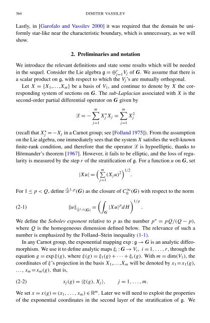
Lastly, in [Garofalo and Vassilev 2000] it was required that the domain be uniformly
star-like near the characteristic boundary, which is unnecessary, as we will
show.
2. Preliminaries and notation
We introduce the relevant definitions and state some results which will be needed
in the sequel. Consider the Lie algebra g = ⊕ r j=1 V j of G. We assume that there is
a scalar product on g, with respect to which the V j ’s are mutually orthogonal.
Let X = {X 1 ,. . . ,X m } be a basis of V 1 , and continue to denote by X the corresponding
system of sections on G. The sub-Laplacian associated with X is the
second-order partial differential operator on G given by
m∑
= − Xj ∗ X j =
j=1
m∑
j=1
X 2 j
(recall that Xj ∗ = −X j in a Carnot group; see [Folland 1975]). From the assumption
on the Lie algebra, one immediately sees that the system X satisfies the well-known
finite-rank condition, and therefore that the operator is hypoelliptic, thanks to
Hörmander’s theorem [1967]. However, it fails to be elliptic, and the loss of regularity
is measured by the step r of the stratification of g. For a function u on G, set
( m∑
|Xu| = (X j u) 2) 1/2
.
j=1
For 1 ≤ p < Q, define ˚1,p (G) as the closure of C0 ∞ (G) with respect to the norm
(∫
1/p
(2-1) ‖u‖ ˚1,p (G) = |Xu| p d H)
.
G
We define the Sobolev exponent relative to p as the number p ∗ = pQ/(Q − p),
where Q is the homogeneous dimension defined below. The relevance of such a
number is emphasized by the Folland–Stein inequality (1-1).
In any Carnot group, the exponential mapping exp : g → G is an analytic diffeomorphism.
We use it to define analytic maps ξ i : G → V i , i = 1, . . . , r, through the
equation g = exp ξ(g), where ξ(g) = ξ 1 (g) + · · · + ξ r (g). With m = dim(V 1 ), the
coordinates of ξ’s projection in the basis X 1 ,. . . ,X m will be denoted by x 1 =x 1 (g),
. . . , x m =x m (g), that is,
(2-2) x j (g) = 〈ξ(g), X j 〉, j = 1, . . . , m.
We set x = x(g) = (x 1 , . . . , x m ) ∈ m . Later we will need to exploit the properties
of the exponential coordinates in the second layer of the stratification of g. We