

Get my PhD Thesis
Get my PhD Thesis
Get my PhD Thesis

You also want an ePaper? Increase the reach of your titles
YUMPU automatically turns print PDFs into web optimized ePapers that Google loves.
<strong>PhD</strong> <strong>Thesis</strong><br />
Optimization of Densities in<br />
Hartree-Fock and Density-functional Theory<br />
Atomic Orbital Based Response Theory<br />
and<br />
Benchmarking for Radicals<br />
Lea Thøgersen<br />
Department of Chemistry<br />
University of Aarhus<br />
2005
"Experiments are the only means of knowledge at our disposal.<br />
The rest is poetry, imagination."<br />
Max Planck
Contents<br />
Preface .........................................................................................................................v<br />
List of Publications ....................................................................................................vii<br />
Part 1 Improving Self-consistent Field Convergence.................................................1<br />
1.1 Introduction .....................................................................................................................1<br />
1.2 The Self-consistent Field Method....................................................................................2<br />
1.3 A Survey of Methods for Improving SCF Convergence .................................................5<br />
1.3.1 Energy Minimization.............................................................................................6<br />
1.3.2 Damping and Extrapolation...................................................................................7<br />
1.3.3 Level Shifting......................................................................................................11<br />
1.4 Development of SCF Optimization Algorithms ............................................................12<br />
1.4.1 Dynamically Level Shifted Roothaan-Hall .........................................................13<br />
1.4.1.1 RH Step with Control of Density Change..............................................13<br />
1.4.1.2 The Trust Region RH Level Shift ..........................................................15<br />
1.4.1.3 DIIS and Dynamically Level Shifted RH ..............................................16<br />
1.4.1.4 Line Search TRRH.................................................................................18<br />
1.4.1.5 Optimal Level Shift without MO Information.......................................19<br />
1.4.1.6 The Trace Purification Scheme..............................................................23<br />
1.4.2 Density Subspace Minimization..........................................................................25<br />
1.4.2.1 The Trust Region DSM Parameterization..............................................25<br />
1.4.2.2 The Trust Region DSM Energy Function ..............................................26<br />
1.4.2.3 The Trust Region DSM Minimization ...................................................27<br />
1.4.2.4 Line Search TRDSM..............................................................................29<br />
1.4.2.5 The Missing Term..................................................................................30<br />
1.4.3 Energy Minimization Exploiting the Density Subspace .....................................32<br />
1.4.3.1 The Augmented RH Energy model........................................................33<br />
1.4.3.2 The Augmented RH Optimization .........................................................34<br />
1.4.3.3 Applications ...........................................................................................36<br />
1.5 The Quality of the Energy Models for HF and DFT .....................................................37<br />
1.5.1 The Quality of the TRRH Energy Model............................................................39<br />
1.5.2 The Quality of the TRDSM Energy Model.........................................................42<br />
1.6 Convergence for Problems with Several Stationary Points...........................................44<br />
1.6.1 Walking Away from Unstable Stationary Points ................................................46<br />
1.6.1.1 Theory....................................................................................................46<br />
1.6.1.2 Examples................................................................................................47<br />
i
1.7 Scaling .......................................................................................................................... 48<br />
1.7.1 Scaling of TRRH ................................................................................................ 49<br />
1.7.2 Scaling of TRDSM ............................................................................................. 51<br />
1.8 Applications.................................................................................................................. 51<br />
1.8.1 Calculations on Small Molecules ....................................................................... 52<br />
1.8.2 Calculations on Metal Complexes...................................................................... 54<br />
1.9 Conclusion .................................................................................................................... 56<br />
Part 2 Atomic Orbital Based Response Theory........................................................ 59<br />
2.1 Introduction................................................................................................................... 59<br />
2.2 AO Based Response Equations in Second Quantization .............................................. 60<br />
2.2.1 The Parameterization.......................................................................................... 60<br />
2.2.2 The Linear Response Function ........................................................................... 62<br />
2.2.3 The Time Development of the Reference State.................................................. 63<br />
2.2.4 The First-order Equation .................................................................................... 64<br />
2.2.5 Pairing................................................................................................................. 66<br />
2.3 Solving the Response Equations................................................................................... 68<br />
2.3.1 Preconditioning................................................................................................... 69<br />
2.3.2 Projections .......................................................................................................... 70<br />
2.4 The Excited State Gradient ........................................................................................... 71<br />
2.4.1 Construction of the Lagrangian .......................................................................... 71<br />
2.4.2 The Lagrange Multipliers ................................................................................... 72<br />
2.4.3 The Geometrical Gradient .................................................................................. 73<br />
2.4.4 The First-order Excited State Properties............................................................. 74<br />
2.5 Test Calculations........................................................................................................... 75<br />
2.6 Conclusion .................................................................................................................... 76<br />
Part 3 Benchmarking for Radicals............................................................................ 77<br />
3.1 Introduction................................................................................................................... 77<br />
3.2 Computational Methods................................................................................................ 77<br />
3.3 Numerical Results......................................................................................................... 79<br />
3.3.1 Convergence of CC and CI Hierarchies ............................................................. 79<br />
3.3.2 The Potential Curve for CN................................................................................ 80<br />
3.3.3 Spectroscopic Constants and Atomization Energy for CN................................. 81<br />
3.3.4 The Vertical Electron Affinity of CN................................................................. 82<br />
3.3.5 The Equilibrium Geometry of CCH ................................................................... 83<br />
3.4 Conclusion .................................................................................................................... 84<br />
ii
Summary....................................................................................................................87<br />
Dansk Resumé ...........................................................................................................89<br />
Appendix A................................................................................................................91<br />
Appendix B................................................................................................................93<br />
Acknowledgements....................................................................................................95<br />
References..................................................................................................................97<br />
iii
Preface<br />
The present <strong>PhD</strong> thesis is the outcome of four years of <strong>PhD</strong> studies at the Faculty of Science,<br />
University of Aarhus, Denmark.<br />
The thesis is divided into three distinct parts which can be read independently. Part 1 deals with the<br />
optimization of the one-electron density in Hartree Fock and density functional theory, and Part 2<br />
deals with atomic orbital based response theory for Hartree Fock and density functional theory. Part<br />
2 thus naturally follows after Part 1. In Part 3 benchmark results from FCI calculations on the<br />
radicals CN and CCH are given.<br />
The work presented in Part 1 has resulted in papers I - III as listed in the following List of<br />
Publications and the work presented in Part 3 has resulted in papers V – VI. The work presented in<br />
Part 2 was initialized in the fall 2004 and will result in paper IV. The development of improved<br />
optimization algorithms for self-consistent field calculations is the subject on which I have spent the<br />
most of <strong>my</strong> time, and Part 1 therefore makes up the larger part of this thesis.<br />
The work has been carried out under the supervision of and in collaboration with Dr. Jeppe Olsen<br />
and Professor Poul Jørgensen at the University of Aarhus. Some work was carried out during visits<br />
at The Royal Institute of Technology in Stockholm, Sweden, the University of Trieste, Italy and the<br />
University of Oslo, Norway. The following people have also contributed to the work presented in<br />
this thesis (see List of Publications): Paweł Sałek (The Royal Institute of Technology in<br />
Stockholm), Sonia Coriani (University of Trieste), Trygve Helgaker (University of Oslo), Stinne<br />
Høst (University of Aarhus), Danny Yeager (Texas A&M University), Andreas Köhn (University of<br />
Aarhus), Jürgen Gauss (University of Mainz), Péter Szalay (Eötvös Loránd University) and Mihály<br />
Kállay (University of Mainz).<br />
The outline of the thesis is as follows: Part 1 is based on the published papers I – II and the<br />
unpublished paper III, but can be read independently of the papers. Certain discussions in the papers<br />
I - II are left out of the thesis and only referred to, as they might as well be read in the papers. Other<br />
discussions not published in the papers are presented in this thesis, including the latest<br />
developments of the algorithms. Part 2 is simply paper IV in preparation. Part 3 is based on the<br />
published papers V – VI and is basically a short version of paper V combined with selected results<br />
from paper VI. Also this part can be read independently of the papers.<br />
v
List of Publications<br />
This thesis includes the following papers. Number I, II, V and VI have already been published and<br />
are attached this thesis, whereas III and IV are in preparation.<br />
Part 1<br />
I. The Trust-region Self-consistent Field Method: Towards a Black Box optimization in Hartree-<br />
Fock and Kohn-Sham Theories,<br />
L. Thøgersen, J. Olsen, D. Yeager, P. Jørgensen, P. Sałek, and T. Helgaker,<br />
J. Chem. Phys. 121, 16 (2004)<br />
II. The Trust-region Self-consistent Field Method in Kohn-Sham Density-functional Theory,<br />
L. Thøgersen, J. Olsen, A. Köhn, P. Jørgensen, P. Sałek, and T. Helgaker,<br />
J. Chem. Phys. 123, 074103 (2005)<br />
III. Augmented Roothaan-Hall for converging Densities in Hartree-Fock and Density-functional<br />
Theory,<br />
S. Høst, L. Thøgersen, P. Jørgensen and J. Olsen<br />
Part 2<br />
IV. Atomic Orbital Based Response Theory,<br />
L. Thøgersen, P. Jørgensen, J. Olsen and S. Coriani<br />
Part 3<br />
V. A Coupled Cluster and Full Configuration Interaction Study of CN and CN - ,<br />
L. Thøgersen and J. Olsen,<br />
Chem. Phys. Lett. 393, 36 (2004)<br />
VI. Equilibrium Geometry of the Ethynyl (CCH) Radical,<br />
P. G. Szalay, L. Thøgersen, J. Olsen, M. Kállay and J. Gauss,<br />
J. Phys. Chem. A 108, 3030 (2004).<br />
vii
Part 1<br />
Improving Self-consistent Field Convergence<br />
1.1 Introduction<br />
The Hartree-Fock (HF) self-consistent field (SCF) method has been around in an orbital formulation<br />
since 1951, where it was introduced by Roothaan 1 and Hall 2 , but today it is as significant as ever.<br />
Even though numerous higher correlated methods with superior accuracy have been developed<br />
since then, most of them still use the Hartree-Fock wave function as the reference function, and are<br />
thus still dependent on a functioning Hartree-Fock optimization. When Kohn and Sham 3 recognized<br />
in 1965 that the Roothaan-Hall SCF scheme had a lot to offer the density optimization in density<br />
functional theory (DFT), the DFT methods entered the chemical scene. Now it was in theory also<br />
possible to obtain results at the exact level from SCF calculations; if only the correct functional<br />
could be found. The developments in computer hardware and linear scaling SCF algorithms over<br />
the last decade have made it possible to carry out ab initio quantum chemical calculations on biomolecules<br />
with hundreds of amino acids and on large molecules relevant for nano-science.<br />
Quantum chemical calculations are thus evolving to become a widespread tool for use in several<br />
scientific branches. It is therefore important that the algorithms work as black-boxes, such that the<br />
user outside quantum chemistry does not have to be concerned with the details of the calculations.<br />
Since no scientific results neither from the higher correlated calculations nor from the large-scale<br />
calculations can be achieved if the SCF optimization does not converge, it is necessary to take an<br />
interest in developing a sound, stable optimization scheme that can handle the complexity in the<br />
problems of the future.<br />
This part of <strong>my</strong> thesis is a contribution to the quest for a black-box SCF optimization algorithm with<br />
optimal convergence properties. In Section 1.2, the basic Hartree-Fock/Kohn-Sham theory and<br />
notation of this part of the thesis is stated, and in Section 1.3 the efforts through the years to<br />
1
Part 1<br />
Improving Self-consistent Field Convergence<br />
improve the Roothaan-Hall SCF scheme are reviewed. Our contributions to the development of<br />
stable and physical sound SCF optimization schemes are presented in Section 1.4, and in Section<br />
1.5 we study the quality of the schemes when applied for HF and DFT. Optimization of problems<br />
with several stationary points is discussed in Section 1.6, in Section 1.7 the scaling of the algorithms<br />
is accounted for, and Section 1.8 contains some convergence examples for HF and DFT calculations<br />
using the algorithms presented in Section 1.4. Finally, Section 1.9 contains concluding remarks;<br />
reviewing the results of this part of the thesis.<br />
1.2 The Self-consistent Field Method<br />
In the following we consider a closed-shell system with N/2 electron pairs. The basic theory of the<br />
Hartree-Fock (HF) and the Kohn-Sham (KS) density optimizations will be described<br />
simultaneously, and the differences will be noted as they appear. Since we are interested in<br />
extending the algorithms presented to large scale calculations, a formulation without reference to<br />
the delocalized molecular orbitals (MOs) is essential, and thus the focus will be on the density in the<br />
atomic orbital (AO) basis rather than the MOs themselves. All through the thesis, SCF will be used<br />
as a general term for HF and KS-DFT methods since they have the SCF optimization scheme in<br />
common. The orbital index convention used in this thesis is i, j, k, l for occupied MOs, a, b, c, d for<br />
virtual MOs, p, q for MOs in general, and Greek letters µ, ν, ρ, σ for AOs.<br />
For closed-shell restricted Hartree-Fock or DFT, the electronic energy is given by<br />
E = 2TrhD + Tr DG( D) + h + E ( D ), (1.1)<br />
SCF nuc XC<br />
where h is the one-electron Hamiltonian matrix in the AO basis, h nuc is the nuclear-nuclear repulsion<br />
contribution, and D is the (scaled) one-electron density matrix in the AO basis, D = ½D AO , which<br />
satisfies the symmetry, trace, and idempotency conditions,<br />
D<br />
T<br />
Tr DS =<br />
= D<br />
N<br />
2<br />
DSD = D ,<br />
(1.2)<br />
of a valid one-electron density matrix. S is the AO overlap matrix. The elements of G(D) are given<br />
by<br />
∑<br />
∑<br />
G ( D ) = 2 g D −γ g D , (1.3)<br />
µν µνρσ ρσ µσρν ρσ<br />
ρσ<br />
ρσ<br />
where g µνρσ are the two-electron AO integrals. The first term in Eq. (1.3) represents the Coulomb<br />
contribution, and the second term is the contribution from exact exchange, with γ = 1 in Hartree-<br />
Fock theory, γ = 0 in pure DFT, and γ ≠ 0 in hybrid DFT. The exchange-correlation energy E XC (D)<br />
in Eq. (1.1) is a nonlinear and non-quadratic functional of the electronic density. This term is only<br />
2
The Self-consistent Field Method<br />
present in the energy expression for the DFT level of theory - the Hartree-Fock energy is expressed<br />
only by the first three terms of Eq. (1.1). The form of E XC depends on the DFT functional chosen for<br />
the calculation.<br />
The first derivative of the electronic energy with respect to the density is found as<br />
where<br />
(1) ∂ESCF<br />
( D)<br />
ESCF<br />
( D) = = 2 F( D)<br />
, (1.4)<br />
∂D<br />
1<br />
2<br />
(1)<br />
XC<br />
FD ( ) = h+ GD ( ) + E ( D )<br />
(1.5)<br />
is the Kohn-Sham matrix in DFT and, if the last term is excluded, the Fock matrix in Hartree-Fock<br />
(1)<br />
theory. From now on F(D) is simply referred to as the Fock matrix. E XC ( D ) is the first derivative<br />
of the term E XC expanded in the density.<br />
The Fock matrix is by design an effective one-electron Hamiltonian which is itself dependent on the<br />
eigenfunctions. Optimizing the electronic energy is thus a nonlinear problem and an iterative<br />
scheme must be applied. In 1951 Roothaan and Hall suggested an iterative procedure 1,2 in which a<br />
set of molecular orbitals (MOs) are constructed in each step through a diagonalization of the current<br />
Fock matrix, which in the AO formulation is written as<br />
FC = SCε , (1.6)<br />
where S is the AO overlap matrix, ε is a diagonal matrix containing the orbital energies, and the<br />
eigenvectors C contain the MO coefficients. The MOs, φ p , are linear combinations of a finite set of<br />
one-electron basis functions, χ µ , with C µp as expansion coefficients<br />
ϕ<br />
p<br />
= ∑ χ C . (1.7)<br />
µ<br />
µ µ p<br />
For the closed shell case the MOs can be divided into an occupied (φ occ ) and a virtual (φ virt ) part,<br />
where the occupied MOs each contain two electrons and the virtual orbitals are empty. If the aufbau<br />
ordering rule is applied, the occupied MOs are chosen as those with the lowest eigenvalues.<br />
A new trial density D can then be constructed from the occupied orbitals as<br />
occ<br />
T<br />
occ<br />
D = C C . (1.8)<br />
From this density a new Fock matrix can be evaluated from Eq. (1.5) and diagonalizing it according<br />
to Eq. (1.6) establishes the iterative procedure. The iterative cycle stops when self-consistency is<br />
obtained, that is, when the new density, energy or molecular orbitals do not change within some<br />
convergence threshold compared to the previous ones.<br />
3
Part 1<br />
Improving Self-consistent Field Convergence<br />
In an iterative scheme it is necessary to have a start guess. For the SCF case it should be a one<br />
electron density which fulfils Eq. (1.2), created directly or from a start guess of the molecular<br />
orbitals as in Eq. (1.8). Different approaches are used; a simple and easily applicable possibility is<br />
to obtain the starting orbitals by diagonalization of the one-electron Hamiltonian (H1-core). This is<br />
the start guess most widely used in this thesis since it is always available. Another popular<br />
possibility is to create a semi-empirical start guess where the orbitals resulting from a semiempirical<br />
calculation (e.g. Hückel) on the molecule are fitted to the current basis.<br />
n = n+1<br />
no<br />
D 0<br />
F(D n<br />
)<br />
F(D n<br />
) D n+1<br />
D n+1<br />
≈ D n<br />
yes<br />
The steps of the self-consistent field (SCF) scheme are summarized<br />
from the density point of view in Fig. 1.1: From a density matrix start<br />
guess a Fock matrix is constructed. From this Fock matrix a new density<br />
matrix can be found and so an iteration procedure is established which<br />
continues until self consistency. The step creating a new density from a<br />
Fock matrix will be referred to as the Roothaan-Hall (RH) step<br />
throughout this thesis, regardless if it is a diagonalization of the Fock<br />
matrix or some alternative scheme.<br />
The purpose of an SCF optimization is typically to find the global<br />
D conv<br />
minimum. Since the HF/KS equations are nonlinear, several stationary<br />
Fig. 1.1 Flow diagram of<br />
points might exist, and depending on the start guess and the<br />
the SCF scheme.<br />
optimization procedure, the converged result can be representing a local<br />
minimum as well as a global or even a saddle point. By evaluating the lowest Hessian eigenvalue it<br />
can be realized whether the stationary point is a minimum or a saddle point, but no simple test can<br />
reveal whether a minimum is global or not. The use of the term “convergence” in this thesis will<br />
simply refer to the iterative development from the start guess to a self-consistent density with a<br />
gradient below the convergence threshold. The issues connected with problems where several<br />
stationary points can be found are discussed in Section 1.6.<br />
Since Roothaan and Hall suggested the iterative diagonalization procedure as a means to solve the<br />
Hartree-Fock equations and Kohn and Sham suggested using the same scheme for optimizing the<br />
electron density for density functional theory 3 , the SCF methods have been used extensively in<br />
quantum chemistry. Unfortunately, it turned out that the simple fixed point scheme sketched in Fig.<br />
1.1 converges only in simple cases. Already around 1960 it was recognized that the method<br />
sometimes fails to converge and that divergent behavior in some cases is intrinsic 4,5 .<br />
4
A Survey of Methods for Improving SCF Convergence<br />
1.3 A Survey of Methods for Improving SCF Convergence<br />
Numerous suggestions have been made to improve upon the convergence of Roothaan and Hall’s<br />
original scheme or to replace it with an alternative scheme. The suggestions can be crudely divided<br />
into three different categories; energy minimization, damping/extrapolation, and level shifting.<br />
Furthermore the different suggestions in these categories have been combined in various ways. The<br />
two latter categories are modifications to the Roothaan-Hall scheme, whereas energy minimization<br />
is a means of avoiding the iterative diagonalization scheme and instead use some optimization<br />
scheme on an energy function.<br />
To <strong>my</strong> knowledge these categories embrace all convergence improvements suggested over the<br />
years, except for the method of fractionally occupying orbitals around the Fermi level 6 which does<br />
not fit in any of the categories. As mentioned, the start guess has a great impact on the optimization,<br />
and a poor start guess with the wrong electron configuration can use many iterations changing to a<br />
more optimal electron configuration and in some cases the proper electron configuration is never<br />
found and the calculation diverges. In the methods using fractional occupations, a number of<br />
orbitals around the Fermi level are allowed to have non-integral occupation. The non-integral<br />
occupations are determined from the Fermi-Dirac distribution which is a function of the<br />
temperature. The non-integral occupations are updated in each iteration, and corrected such that the<br />
total number of electrons is constant. During the optimization either the temperature is decreased to<br />
T = 0K or the number of orbitals allowed to have non-integral occupation is decreased, to have only<br />
integer occupations at the end of the optimization. It is thus possible to optimize the electron<br />
configuration in an effective manner in the beginning of the SCF optimization, and when the proper<br />
configuration has been found, the rest of the optimization has a better chance of convergence since<br />
the start guess in a way has been improved.<br />
In the following, the focus will be on the efforts to improve the convergence behavior of the SCF<br />
scheme through optimization algorithm development in the three categories listed above. Other<br />
efforts bear as much significance and should also be acknowledged, in particular should be<br />
mentioned the generalizations of many well-functioning schemes to the unrestricted level of theory<br />
which has its own challenges. Also the quest for construction of an improved start guess is<br />
important. It is obvious that with an improved start guess, less is demanded from the optimization<br />
method and thus some convergence problems inherent in the methods could be avoided. In the last<br />
decade the effort in SCF scheme development has for a large part been put in decreasing the scaling<br />
of the methods to allow calculations on larger molecules. Scaling is a very important subject and it<br />
should not be ignored. Section 1.7 will therefore discuss the scaling of the algorithms presented in<br />
5
Part 1<br />
Improving Self-consistent Field Convergence<br />
this thesis. Despite the importance of these three SCF related subjects, the rest of this section will be<br />
almost solely on efforts to improve convergence through optimization algorithm development.<br />
1.3.1 Energy Minimization<br />
One of the problems in the simple Roothaan-Hall procedure is the lack of guarantees for energy<br />
decrease in the iterative steps. This was pointed out by McWeeny, and he thus introduced a steepest<br />
descent procedure 7,8 as an energy minimization alternative to Roothaan and Hall’s repeated<br />
diagonalizations. Steepest descent optimizations have the benefit that a decrease in energy can be<br />
guaranteed for each step. McWeeny’s scheme suffers, however, from a slow convergence rate 5 as<br />
often seen for steepest descent methods. Fletcher and Reeves proposed the conjugate gradient<br />
optimization method 9 instead, which often is more efficient than steepest descent and is guaranteed<br />
to converge in a number of steps equal to the dimension of the problem.<br />
A decade later Hilliers and Saunders suggested an improvement to the McWeeny scheme called<br />
energy-weighted steepest descent 10 , in which the coordinates in the orbital space are energyweighted.<br />
In 1976 this work was generalized by Seeger and Pople. They realized that another<br />
problem in the simple Roothaan procedure is the possibility for discontinuous changes in the<br />
orbitals which do not necessarily lower the energy. To ensure energy descent it is necessary to be<br />
able to follow such changes continuously, and methods like the steepest descent have the possibility<br />
to do so. Their procedure proceeds in small steps, where the new occupied trial orbitals are selected<br />
based on a criterion of overlap with the previous set. This technique ensures stability and avoids<br />
switching of orbital occupation. The step is found by a univariate search 11 in the energy, on a path<br />
that passes through the point corresponding to the next iteration step of the classical procedure.<br />
Their scheme can therefore also be seen as a polynomial interpolation along a path joining<br />
successive SCF cycles. Half a decade later, Camp and King followed the same strategy of a<br />
univariant cubic fit technique 12 , but with a different parameterization. Stanton also suggested a<br />
similar approach 13 , but whereas the Seeger-Pople approach requires the evaluation of the Fock<br />
matrix at interior points on the interpolative path, Stanton’s scheme uses a cubic interpolation,<br />
where only the end point properties are needed, making it a less expensive method.<br />
Another way of improving the convergence properties is to evaluate the gradient and Hessian of the<br />
electronic energy analytically with respect to some variational parameter, and then optimize the<br />
energy through Newton-Raphson steps resulting in a quadratically convergent 14 scheme, at least in<br />
the region close to the optimized state where a second order approximation is reasonable. These<br />
methods are computationally very expensive since a four index transformation is required to obtain<br />
the Hessian information. In 1981 Bacskay proposed a quadratically convergent SCF (QC-SCF)<br />
method 15 which escapes the four index transformation while requiring four or five micro iterations<br />
6
A Survey of Methods for Improving SCF Convergence<br />
per step (in non-problematic cases), each of which is about as expensive computationally as<br />
building a Fock matrix. His method was inspired from single excitation configuration interaction<br />
(SX-CI) and multi-configurational SCF (MC-SCF). A possible divergence of the scheme can be<br />
overcome by moderating the orbital update step by the augmented Hessian method 16 or trust radius<br />
techniques 17 . Even though it is still quite expensive, the method is also used today for cases with<br />
convergence problems, since a decrease in energy can be ensured step by step and it has quadratic<br />
convergence properties near the optimized state.<br />
Around 1995, the interest for linear scaling SCF methods took on, since the development in<br />
computer hardware had made calculations on large molecules possible. With newly developed<br />
algorithms the evaluation of the Fock matrix, with the formal scaling of N 4 arising from the fourindex<br />
integrals, could now routinely be decreased to a near-linear scaling. The diagonalization with<br />
a N 3 scaling in standard Roothaan-Hall was now the bottle neck. Inspiration was found in tight<br />
binding theory 18-20 , where a number of linear scaling approaches had been suggested earlier 21 . To<br />
obtain linear scaling of the RH step it is necessary to avoid the diagonalization and to ensure<br />
sparsity in the matrices. This is a problem since the convenient canonical MO basis is inherently<br />
delocalized. Some of the well known schemes were reformulated in localized MOs 22 , while others<br />
developed strict AO formulations 20,23-25 . Most of the suggested linear scaling methods did not arise<br />
so much to improve convergence as to improve the scaling, and will therefore not be discussed in<br />
further detail.<br />
Very recently Francisco, Martínez and Martínez introduced their globally convergent trust region<br />
methods for SCF 26 , where the standard fixed-point Roothaan-Hall step is replaced by a trust region<br />
optimization of a model energy function. This algorithm has very nice features since it can be<br />
proved to be globally convergent, and the step sizes are controlled dynamically through a trust<br />
region update scheme. The convergence rate seems rather random though; sometimes perfect and<br />
sometimes hopeless, but only small test examples have been published, so time will show.<br />
1.3.2 Damping and Extrapolation<br />
In his SCF study of atoms, Hartree noted convergence difficulties and suggested a so-called<br />
damping scheme 27 as a modification to the iterative procedure. Instead of using the newly<br />
constructed density D n+1 , which corresponds to a full step, a linear combination of the new density<br />
matrix with the previous one is constructed<br />
damp<br />
Dn+ 1<br />
= Dn + λ( Dn+ 1 − Dn ) = λDn+<br />
1 + ( 1 −λ)<br />
D n , (1.9)<br />
7
Part 1<br />
Improving Self-consistent Field Convergence<br />
where λ – the damping factor - is a scalar chosen between zero and one. The iterative sequence is<br />
then continued with D damp as the new density. Hartree found that this scheme could force<br />
convergence in problematic cases.<br />
To get an idea of the effect of the damping factor, we consider a block-diagonal Fock matrix in the<br />
MO basis<br />
F<br />
MO<br />
⎛ εo<br />
Fov<br />
⎞<br />
= ⎜ ⎟ , (1.10)<br />
⎝Fvo<br />
εv<br />
⎠<br />
where ‘o’ denotes occupied, ‘v’ virtual and [ε o ] ij = δ ij ε i and [ε v ] ab = δ ab ε a . The change in electronic<br />
energy from the first order variation of the occupied orbitals through first-order perturbation theory<br />
is then given as<br />
virtual occupied 2<br />
( 1)<br />
−Fai<br />
SCF<br />
4<br />
a i<br />
εa<br />
− εi<br />
∆ E =<br />
∑ ∑ . (1.11)<br />
( )<br />
If this first order term is negative and sufficiently small such that the higher order contributions are<br />
insignificant, then a decrease in the electronic energy is seen. If the MOs obey the aufbau principle,<br />
then all ε i < ε a and it is clear that the term is negative as desired. The Hartree damping of Eq. (1.9)<br />
roughly corresponds to multiplying the numerator of Eq. (1.11) by the factor λ, which is positive<br />
and less than one<br />
virtual occupied 2<br />
( 1)<br />
−λFai<br />
SCF<br />
4<br />
a i<br />
εa<br />
− εi<br />
∆ E =<br />
∑ ∑ , (1.12)<br />
( )<br />
thus giving the opportunity to obtain a negative first order change of arbitrarily small magnitude,<br />
making the higher order terms insignificant. Though this would seem promising, the aufbau<br />
principle is seldom obeyed all through the optimization.<br />
If λ could be freely chosen, the damping technique would lead to an extrapolation scheme in the<br />
densities. Since SCF generates an iterative sequence where each step only depends upon the<br />
preceding, it was natural to apply the mathematical extrapolation methods (e.g. the Aitken<br />
extrapolation 28 procedures) on SCF to improve in particular the convergence rate close to the<br />
minimum. When the individual MO expansion coefficients are chosen as the extrapolated<br />
parameters, as Winter and Dunning Jr. 29 suggested, unphysical result may be obtained, though they<br />
can be corrected at the end of the calculation. Nielsen used instead the density matrix as the<br />
extrapolated parameter 30 and an eigenvalue extrapolation instead of the Aitken method. This led to a<br />
scheme more similar to Hartree damping, but with λ found within the eigenvalue extrapolation<br />
scheme.<br />
8
A Survey of Methods for Improving SCF Convergence<br />
Different approaches have been taken to dynamically find the damping factor λ. Zerner and<br />
Hehenberger 31 found it based on an extrapolation of the Mulliken gross population. Karlström 32<br />
expressed the electronic energy in the damped density E(D damp ) and used the first derivative with<br />
respect to λ, to choose in each iteration the λ that minimized the electronic energy.<br />
None of these schemes were very successful solving the convergence problems. They all had some<br />
particular problematic cases they could handle better than the predecessors, but in general they did<br />
not catch on. Pulay then suggested in the early 1980s to use the norm of a linear combination of<br />
error vectors e i from the individual iterations, where the vanishing of the error vector is a necessary<br />
and sufficient condition for SCF convergence. The norm is then optimized with respect to the<br />
coefficients c i<br />
n<br />
e ( c)<br />
= ∑ ciei<br />
, (1.13)<br />
where n is the number of previous iterations, and the coefficients are restricted to add up to 1<br />
n<br />
i=<br />
1<br />
i=<br />
1<br />
∑ ci<br />
= 1. (1.14)<br />
The resulting coefficients are used to construct a favorable linear combination of the previous Fock<br />
matrices<br />
n<br />
F = ∑ ciF i , (1.15)<br />
i=<br />
1<br />
which is diagonalized to obtain a new density, and so the iterative procedure is reestablished. This<br />
was the first density subspace minimization scheme that deliberately exploited the information<br />
obtained in the previous iterations and he named the approach DIIS 33 for “Direct Inversion in the<br />
Iterative Subspace”. For the special case of two matrices, the DIIS density corresponds to the<br />
damped density of Eq. (1.9), but with no restrictions on λ. A decade later the DIIS algorithm was a<br />
standard option in most ab initio programs and had effectively solved a number of the convergence<br />
problems. The orbital rotation gradient was typically used as the error vector for wave function<br />
optimizations, and Sellers pointed out 34 that the DIIS algorithm exploits the second-order<br />
information contained in a set of gradients to obtain quadratic convergence behavior. Some<br />
numerical problems were seen though, where numerical instabilities appeared because of linear<br />
dependencies in the space of error vectors. Sellers introduced the C2-DIIS method 34 , which is<br />
similar to DIIS except the restriction is on the squares of the coefficients<br />
n<br />
2<br />
∑ ci<br />
= 1 , (1.16)<br />
i=<br />
1<br />
9
Part 1<br />
Improving Self-consistent Field Convergence<br />
with a renormalization at the end. This gives an eigenvalue problem to be solved instead of the set<br />
of linear equations in normal DIIS, and thus singularities are more easily handled. However, one of<br />
the examples (Pd 2 in the Hyla-Kripsin basis set 35 ) given in ref. 34 , where DIIS supposedly diverges,<br />
converges for our plain DIIS implementation to 10 -7 in the energy in 14 iterations.<br />
Even though DIIS is successful, examples of divergence with no relation to numerical instabilities<br />
have been encountered over the years. In the year 2000 Cancès and Le Bris presented a damping<br />
algorithm named the Optimal damping Algorithm 36 (ODA) that ensures a decrease in energy at each<br />
iteration and converges toward a solution to the HF equations. In ODA the damping factor λ is<br />
found based on the minimum of the Hartree-Fock energy for the damped density in Eq. (1.9)<br />
E<br />
damp<br />
( Dn+<br />
1<br />
, λ) = E ( Dn ) + 2λTrF( Dn )( Dn+<br />
−Dn<br />
)<br />
HF HF 1<br />
2<br />
+ λ Tr ( D −D ) G( D − D ) + h ,<br />
n+ 1 n n+<br />
1 n nuc<br />
(1.17)<br />
much like Karlström did it in 1979. The damping factor is thus optimized in each iteration, hence<br />
the name of the algorithm.<br />
Recently Kudin, Scuseria, and Cancès proposed a method in which the gradient-norm minimization<br />
in DIIS is replace by a minimization of an approximation to the true energy function and they<br />
named it the energy DIIS (EDIIS) method 37 . Where the ODA used the energy expression of Eq.<br />
(1.17) to find the optimal λ, EDIIS uses an approximation of the Hartree-Fock energy for the<br />
averaged density<br />
n<br />
EDIIS 1<br />
n<br />
D = ∑ ciD i , (1.18)<br />
i=<br />
1<br />
( , ) = ∑ i SCF ( i ) −<br />
2 ∑ i j Tr( ( i − j ) ⋅( i − j ))<br />
i= 1 i, j=<br />
1<br />
n<br />
E Dc c E D c c F F D D , (1.19)<br />
where the sum of the coefficients c i is still restricted to 1. They combine the scheme with DIIS, such<br />
that the EDIIS optimized coefficients are used to construct the averaged Fock matrix if all<br />
coefficients fall between 0 and 1. If not, the coefficients from the DIIS scheme are used instead. The<br />
EDIIS scheme introduces some Hessian information not found in DIIS and thus improves<br />
convergence in cases where the start guess has a Hessian structure far from the optimized one. For<br />
non-problematic cases and near the optimized state EDIIS has a slower convergence rate than DIIS,<br />
but it has been demonstrated that EDIIS can converge cases where DIIS diverges.<br />
Recently, we suggested another subspace minimization algorithm along the same line as EDIIS, but<br />
with a smaller idempotency error in the energy model and the same orbital rotation gradient in the<br />
subspace as the SCF energy (the EDIIS energy model actually has a different gradient). We named<br />
it TRDSM 38 for trust region density subspace minimization since a trust region optimization is<br />
10
A Survey of Methods for Improving SCF Convergence<br />
carried out of the energy model in the subspace of previous densities. In the second paper on<br />
TRDSM 39 , a comparison with the EDIIS and DIIS models can be found stating explicitly that the<br />
EDIIS energy model does not have the correct gradient and is wrong for other reasons as well at the<br />
DFT level of theory.<br />
Many of the energy minimization techniques can be combined with a damping or extrapolation<br />
scheme to improve the convergence. Typically, DIIS has been the choice 24,40,41 , but TRDSM could<br />
be used just as well.<br />
1.3.3 Level Shifting<br />
In 1973 Saunders and Hillier introduced the level shift concept 42 . They suggested adding a positive<br />
scalar µ to the diagonal of the virtual-virtual block of the Fock matrix in the MO basis, Eq. (1.10),<br />
before diagonalizing<br />
MO<br />
MO<br />
( µ ( ) )<br />
F + I− D C = Cε , (1.20)<br />
where I is the identity matrix and D MO is the scaled one-electron density matrix in the MO basis<br />
with 1 in the diagonal of the occupied-occupied block and zeros for the rest.<br />
To compare level shifting with the damping scheme of Hartree 27 , consider the first order variation in<br />
the energy change as in Eq. (1.11); the level shift µ then corresponds to adding a positive constant to<br />
the denominator<br />
virtual occupied 2<br />
( 1)<br />
−Fai<br />
SCF<br />
4<br />
a i a i<br />
∆ E =<br />
∑ ∑ . (1.21)<br />
( ε − ε + µ )<br />
The level shift thus has, as the damping factor, the possibility to decrease the magnitude of the term.<br />
The problems with respect to the aufbau principle mentioned in connection with the damping can be<br />
overcome with the level shift. The level shift can separate the occupied orbitals from the virtuals<br />
and thereby ensure a positive denominator and an overall decrease in energy. As the level shift is<br />
increased towards infinity, the obtained decrease in energy will correspond to that of the steepest<br />
descent method as explained in Section 1.4.1.4, and thus the convergence will be slow. This<br />
connection between a large gap between the occupied and the virtual orbitals (HOMO-LUMO gap)<br />
and slow convergence was exploited by Bhattacharyya in 1978 to accelerate convergence for cases<br />
with large HOMO-LUMO gaps. His “reverse level shift” technique 43 uses a negative level shift<br />
instead of a positive, thus decreasing the gap and accelerating the convergence.<br />
In 1977, Carbó, Hernández and Sanz claimed unconditional convergence for an SCF process with a<br />
properly used level shift 44 , and two decades later, Cancès and Le Bris 45 made a formal proof that for<br />
11
Part 1<br />
Improving Self-consistent Field Convergence<br />
any initial guess D 0 , there exists a level shift µ 0 > 0 such that for level shift parameters µ > µ 0 , the<br />
energy decreases at each step and converges towards a stationary value.<br />
The level shift technique is still routinely used for cases where the DIIS scheme has problems. The<br />
level shifts are typically found on a trial and error basis. Recently, we advocated the use of a level<br />
shift to control the changes introduced in the Roothaan-Hall step 38 , and we suggested a way of<br />
optimizing the level shift at each iteration based on physical arguments and without guesswork. The<br />
algorithm is based on the trust region philosophy in which a model energy function is optimized,<br />
but restricted with respect to the step length. We thus named the algorithm trust region Roothaan-<br />
Hall (TRRH), even though it is not a true trust region optimization scheme like e.g. the energy<br />
minimization of Francisco, Martínez, and Martínez 26 or our TRDSM scheme 38 .<br />
Level shifting can be combined with a damping or extrapolation scheme. When the TRRH approach<br />
is combined with the subspace minimization method TRDSM it seems to outperform DIIS in<br />
stability and to have a better or similar convergence rate, as will be illustrated in the following<br />
sections. Combining level shifting with DIIS can occasionally be a benefit, but typically DIIS and<br />
level-shifting does not work well together, and in Section 1.4.1.3 we will try to justify this.<br />
1.4 Development of SCF Optimization Algorithms<br />
The SCF scheme as it typically looks today is sketched in Fig. 1.2. Compared to Fig. 1.1, the step <br />
is inserted, illustrating a density subspace minimization, where<br />
some function f is minimized with respect to the coefficients c i<br />
which expand the previous densities D i . The function f could<br />
be the gradient norm as in DIIS or some energy model<br />
D 0<br />
F(D n<br />
)<br />
n<br />
approximating the SCF energy in the subspace of the previous<br />
D = ∑ciDi,minf<br />
( c)<br />
densities as in EDIIS and TRDSM. In the Roothaan-Hall step<br />
i=<br />
1<br />
<br />
, the averaged Fock matrix F found from the optimization in<br />
n<br />
n = n+1 F =<br />
is then used instead of the most recent Fock matrix F(D n ) to<br />
∑ciF( Di)<br />
i=<br />
1<br />
find a new trial density D n+1 . In general, the averaged density<br />
matrix D is not idempotent and therefore does not represent a<br />
valid density matrix; moreover, since the Kohn-Sham matrix<br />
F D n+1 <br />
(unlike the Fock matrix) is nonlinear in the density matrix, the<br />
averaged Kohn-Sham matrix F is different from FD. ( ) For<br />
these reasons, the averaged Fock matrix F cannot be<br />
no<br />
D n+1<br />
≈ D n<br />
yes<br />
D conv<br />
associated uniquely with a valid Fock matrix. Usually, this<br />
Fig. 1.2 Flow diagram of the SCF<br />
does not matter much since the subsequent diagonalization of scheme including the density<br />
the Fock matrix nevertheless produces a valid density matrix subspace minimization step.<br />
12
Development of SCF Optimization Algorithms<br />
according to Eq. (1.8). The complications arising from the use of the averaged Fock matrix is<br />
disregarded in the following, noting that the errors introduced by this approach may easily be<br />
corrected for, if necessary.<br />
The rest of this part of the thesis will focus on the work we have done over the last couple of years<br />
to improve SCF convergence. We have made developments in all of the three categories of the<br />
previous section. The density subspace minimization scheme TRDSM and the level shift scheme in<br />
TRRH, both briefly described in the previous section, make up a total scheme we have named<br />
TRSCF, where each SCF iteration contains a TRDSM and a TRRH step. The first subsection will<br />
go into further detail on TRRH and will thus be concerned with our modifications to step in Fig.<br />
1.2. The second subsection will likewise go into further detail on TRDSM and will describe the<br />
scheme we apply in step . In the third subsection, a recently developed energy minimization<br />
procedure will be presented. The procedure merges step and integrating a subspace<br />
minimization in the optimization of a new trial density.<br />
This section will primarily take the Hartree-Fock point of view, acknowledging that with small<br />
adjustments and the word Fock replaced by Kohn-Sham, it would describe the DFT situation as<br />
well. In Section 1.5 the differences appearing when the algorithms are applied to the HF and DFT<br />
cases, respectively, will be discussed.<br />
1.4.1 Dynamically Level Shifted Roothaan-Hall<br />
The problems inherent to the RH diagonalization method are the discontinuous changes in the<br />
density and the lack of guarantees for energy decrease. To overcome these problems, we introduced<br />
in 2004 a means to restrict the RH step to the trust region of the RH energy model, with the purpose<br />
of both controlling the changes in the density and ensuring an energy decrease. Since then, the same<br />
ideas have been put forward by Francisco et. al. 26 as well, suggesting a trust region optimization of<br />
a RH energy model.<br />
In this section, our trust region Roothaan-Hall scheme and related subjects are discussed. In<br />
particular, we present two different schemes for dynamic level shifting and an alternative to<br />
diagonalization.<br />
1.4.1.1 RH Step with Control of Density Change<br />
The solution of the traditional Roothaan–Hall eigenvalue problem Eq. (1.6) may be regarded as the<br />
minimization of the sum of the energies of the occupied MOs 8,46<br />
RH<br />
subject to MO orthonormality constraints<br />
E<br />
∑<br />
( D) = 2 ε = 2TrF D (1.22)<br />
i<br />
i<br />
0<br />
13
Part 1<br />
Improving Self-consistent Field Convergence<br />
T<br />
occ occ = N<br />
C SC I , (1.23)<br />
where F 0 is typically obtained as a weighted sum of the previous Fock matrices such as F in Eq.<br />
(1.15). Since Eq. (1.22) represents a crude model of the true Hartree-Fock energy (with the same<br />
first-order term, but different zero- and second-order terms), it has a rather small trust radius. A<br />
global minimization of E RH (D), as accomplished by the solution of the Roothaan–Hall eigenvalue<br />
problem Eq. (1.6), may therefore easily lead to steps that are longer than the trust radius and hence<br />
unreliable. To avoid such steps, we shall impose on the optimization of Eq. (1.22) the constraint that<br />
the new density matrix D does not differ much from the old D 0 , that is, the S-norm of the density<br />
difference should be equal to a small number ∆<br />
2<br />
2<br />
D− D0 S<br />
= Tr ( D−D0 ) S( D− D0 ) S = − 2Tr D0SDS + N = ∆, (1.24)<br />
where N is the number of electrons – see Eq. (1.2) – and the S-norm used throughout this thesis is<br />
defined as<br />
2<br />
S<br />
A = Tr ASAS (1.25)<br />
for symmetric A. The optimization of Eq. (1.22) subject to the constraints Eq. (1.23) and Eq. (1.24)<br />
may be carried out by introducing the Lagrangian<br />
1<br />
T<br />
L = 2TrFD 0 −2µ<br />
( TrDSDS 0 − ( N −∆)<br />
) −2Trη( CoccSCocc<br />
−I N ) , (1.26)<br />
2<br />
where µ is the undetermined multiplier associated with the constraint Eq. (1.24), whereas the<br />
symmetric matrix η contains the multipliers associated with the MO orthonormality constraints.<br />
Differentiating this Lagrangian with respect to the MO coefficients and setting the result equal to<br />
zero, we arrive at the level-shifted Roothaan–Hall equations:<br />
( F − µ SD S) C ( µ ) = SC ( µ ) λ ( µ ). (1.27)<br />
0 0 occ occ<br />
Since the density matrix, Eq. (1.8), is invariant to unitary transformations among the occupied MOs<br />
in C occ ( µ ), we may transform this eigenvalue problem to the canonical basis:<br />
( F − µ SD S) C ( µ ) = SC ( µ ) ε ( µ ) , (1.28)<br />
0 0 occ occ<br />
where the diagonal matrix ε(µ) contains the orbital energies. Note that, since D 0 S projects onto the<br />
part of C occ that is occupied in D 0 (see ref. 46 ), the level-shift parameter µ shifts only the energies of<br />
the occupied MOs. Therefore, the role of µ is to modify the difference between the energies of the<br />
occupied and virtual MOs - in particular, the HOMO–LUMO gap.<br />
Clearly, the success of the trust region Roothaan–Hall (TRRH) method will depend on our ability to<br />
make a judicious choice of the level-shift parameter µ in Eq. (1.28). In our standard TRRH<br />
implementation, we determine µ by requiring that D(µ) does not differ much from D 0 in the sense of<br />
2<br />
14
Development of SCF Optimization Algorithms<br />
Eq. (1.24), thereby ensuring a continuous and controlled development of the density matrix from the<br />
initial guess to the converged one.<br />
1.4.1.2 The Trust Region RH Level Shift<br />
The constraint on the change in the AO density Eq. (1.24) refers to a change which may arise not<br />
only from small changes in many MOs but also from large changes in a few MOs or even in a<br />
single MO. To obtain a high level of control, we shall require that the changes in the individual<br />
new<br />
MOs are all small. Expanding the MOs ϕ i , obtained by diagonalization of Eq. (1.28), in the old<br />
MOs, we obtain<br />
occ<br />
virt<br />
new old new old old new old<br />
i = j i j + a i a<br />
j<br />
a<br />
∑ ∑ , (1.29)<br />
ϕ ϕ ϕ ϕ ϕ ϕ ϕ<br />
where the first summation is over the occupied MOs and the second over the virtual MOs. The<br />
new<br />
squared norm of the projection of ϕ i onto the MO space associated with D 0 is therefore<br />
orb old new<br />
i j i<br />
j<br />
2<br />
a = ∑ ϕ ϕ . (1.30)<br />
To ensure small individual MO changes in each iteration (to within a unitary transformation of the<br />
occupied MOs), we shall therefore require<br />
orb orb orb<br />
min<br />
min i<br />
i<br />
min<br />
a = a ≥ A , (1.31)<br />
orb<br />
where Amin<br />
is close to one (0.98 or 0.975 in practice). This way of controlling the changes in the<br />
density was also used by Seeger and Pople in their steepest descent method 11 .<br />
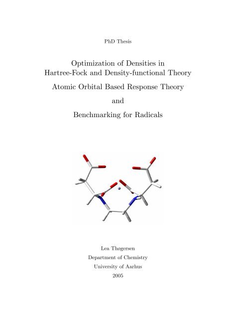
To illustrate how this scheme is used in practice, detailed<br />
information from the TRRH step in iteration 7 of a HF/6-31G and<br />
an LDA/6-31G calculation on the zinc complex depicted in Fig.<br />
1.3 is displayed in Fig. 1.4 and Fig. 1.5, respectively. In the upper<br />
orb orb<br />
panels is illustrated how a search for amin<br />
= Amin<br />
determines the<br />
optimal level shift µ for the TRRH step. The TRRH energy model<br />
is more accurate for HF than for DFT (see Section 1.5.1), and<br />
consequently larger changes can be handled in the TRRH step for Fig. 1.3 Zn 2+ in complex with<br />
orb<br />
ethylenediamine-N,N'-disuccinic<br />
HF than for DFT. A<br />
min<br />
is thus set to 0.975 for HF and 0.98 for<br />
acid (EDDS).<br />
DFT. In the lower panels is seen that the chosen level shifts avoid<br />
an increase in the energy which would have been the case if the Roothaan-Hall step was not level<br />
shifted (µ = 0). Notice also that an even lower energy would have been obtained by reducing the<br />
level shift, but then the restrictions on the overlap should be loosened, and this would result in<br />
15
Part 1<br />
Improving Self-consistent Field Convergence<br />
energy increase in other iterations. In short, the identification of µ from the overlap requirement<br />
a<br />
orb<br />
min<br />
orb<br />
min<br />
= A appears to be a good and secure way to control the step sizes in the optimization.<br />
orb<br />
a min<br />
1.0<br />
0.8<br />
orb<br />
A min = 0.975<br />
orb<br />
a min<br />
1.0<br />
0.8<br />
orb<br />
A min = 0.98<br />
0.6<br />
0.6<br />
0.4<br />
0.2<br />
0.0<br />
A<br />
0 2 4 6 8 10<br />
µ<br />
0.4<br />
0.2<br />
0.0<br />
A<br />
0 2 4 6 8 10<br />
µ<br />
40.0<br />
20.0<br />
RH<br />
∆E HF<br />
40.0<br />
20.0<br />
RH<br />
∆E LDA<br />
∆E / a.u.<br />
0.0<br />
-20.0<br />
-40.0<br />
RH<br />
∆E<br />
0 2 4 6 8 10<br />
µ<br />
Fig. 1.4 HF/6-31G, iteration 7. (A) The overlap<br />
orb<br />
RH<br />
a<br />
min<br />
and (B) the changes in the HF energy ∆ E HF<br />
RH<br />
and in the RH energy model ∆ E as a function of<br />
the level shift µ.<br />
B<br />
∆E / a.u.<br />
0.0<br />
-20.0<br />
-40.0<br />
∆E RH<br />
0 2 4 6 8 10<br />
µ<br />
Fig. 1.5 LDA/6-31G, iteration 7. (A) The overlap<br />
orb<br />
a<br />
min<br />
and (B) the changes in the LDA energy<br />
RH<br />
RH<br />
∆ E LDA<br />
and in the RH energy model ∆ E as a<br />
function of the level shift µ.<br />
B<br />
1.4.1.3 DIIS and Dynamically Level Shifted RH<br />
For accelerating the SCF convergence, DIIS is a simple and in general very successful scheme. We<br />
would expect to get an even better performance and improve the stability of the scheme if DIIS was<br />
combined with a dynamically level shifted RH step like TRRH instead of the standard RH with no<br />
control of the step. To investigate how a combination of DIIS and TRRH performs, we carried out a<br />
number of DIIS-TRRH optimizations. A typical example is seen in Fig. 1.7 and an extraordinary<br />
example is seen in Fig. 1.8.<br />
Fig. 1.6 Cd 2+ complexed with an<br />
imidazole ring.<br />
16
Development of SCF Optimization Algorithms<br />
Error in energy / E h<br />
1.E+02<br />
1.E+00<br />
1.E-02<br />
1.E-04<br />
1.E-06<br />
1.E-08<br />
DIIS<br />
DIIS-TRRH<br />
TRSCF<br />
0 5 10 15 20 25<br />
Iteration<br />
Fig. 1.7 LDA/STO-3G calculations with a H1-core<br />
start guess on the cadmium complex in Fig. 1.6.<br />
Error in energy / E h<br />
1.E+02<br />
1.E+00<br />
1.E-02<br />
1.E-04<br />
1.E-06<br />
TRSCF<br />
DIIS-TRRH<br />
DIIS<br />
0 5 10 15 20 25 30<br />
Iteration<br />
Fig. 1.8 LDA/STO-3G calculations with a Hückel<br />
start guess on the zinc complex in Fig. 1.3.<br />
Somewhat surprisingly the calculations rarely converge with the DIIS-TRRH method. To<br />
understand this behavior, we note that, in the global region, the TRRH method typically produces<br />
gradients that do not change much, even though large changes may occur in the energy. In such<br />
cases, the DIIS method may stall, not being able to identify a good combination of density matrices.<br />
This behavior is illustrated in Table 1-1, where the gradient norm and Kohn–Sham energy of the<br />
first six iterations of the cadmium complex calculations in Fig. 1.7 are listed.<br />
Table 1-1. The Gradient norm ||g||=||4(SDF-FDS)|| in the first six<br />
iterations of the cadmium complex calculations of Fig. 1.7.<br />
DIIS DIIS-TRRH TRSCF<br />
It. E KS ||g|| E KS ||g|| E KS ||g||<br />
1 -5597.0 7.8 -5597.0 7.8 -5597.0 7.8<br />
2 -5502.3 14.9 -5598.4 7.2 -5598.3 7.1<br />
3 -5602.1 9.7 -5600.3 8.5 -5603.7 9.3<br />
4 -5628.5 2.1 -5599.9 7.7 -5611.1 9.1<br />
5 -5627.4 3.5 -5599.9 7.8 -5616.8 7.7<br />
6 -5628.8 0.8 -5600.2 8.1 -5622.7 7.5<br />
conv no conv conv<br />
The TRSCF and DIIS-TRRH gradients stay almost the same during these iterations, stalling the<br />
DIIS-TRRH optimization but not the TRSCF optimization, whose energy decreases in each<br />
iteration. In the pure DIIS optimization, by contrast, the gradient changes significantly from<br />
iteration to iteration; at the same time, the energy decreases at each iteration except the second and<br />
fifth, where also the gradient norms increase. Eventually, DIIS enters the local region with its rapid<br />
rate of convergence although we note a sudden, large increase in the energy in iterations 10 and 11.<br />
However, these changes are accompanied with large increases in the gradient norm, allowing DIIS<br />
to recover safely.<br />
17
Part 1<br />
Improving Self-consistent Field Convergence<br />
In the example Fig. 1.8 standard DIIS diverges. TRSCF converges, but a minimum level shift of 0.1<br />
is used all through the calculation. When DIIS is combined with TRRH in this case, also using a<br />
minimum level shift of 0.1, it converges as well as TRSCF. Table 1-2 contains the gradient norm<br />
and Kohn-Sham energy of the first six iterations of the calculations in Fig. 1.8.<br />
Table 1-2. The gradient norm ||g||=||4(SDF-FDS)|| in the first six<br />
iterations of the zinc complex calculations of Fig. 1.8.<br />
DIIS DIIS-TRRH TRSCF<br />
It. E KS ||g|| E KS ||g|| E KS ||g||<br />
1 -2826.95 11.6 -2826.95 11.6 -2826.95 11.6<br />
2 -2745.49 24.0 -2830.11 3.3 -2830.06 3.4<br />
3 -2809.38 13.6 -2831.04 1.6 -2831.11 1.5<br />
4 -2819.16 9.7 -2831.44 0.8 -2831.42 1.1<br />
5 -2776.74 15.4 -2831.34 1.5 -2831.40 1.5<br />
6 -2826.55 7.0 -2831.41 1.5 -2831.47 0.9<br />
no conv conv conv<br />
In this case the gradient norms for the TRSCF calculation change significantly and a decrease in<br />
gradient relates directly to a decrease in the energy, where in the first example there were no direct<br />
connection between the gradient norm and the energy. The DIIS-TRRH calculation follows the<br />
same gradient behavior as TRSCF, just as in the first example, and they both converge. The DIIS<br />
gradient norm changes, but does not decrease as in the first example. There is still the connection<br />
between small gradients and low energies though, so why DIIS cannot find the proper directions in<br />
this case is not evident.<br />
In our experience DIIS should not be used in connection with a dynamic level shift scheme like<br />
TRRH, since for all but the simplest cases DIIS-TRRH diverged if DIIS converged. We<br />
encountered, however, the example in Fig. 1.8 where DIIS does not converge and DIIS-TRRH does,<br />
but it was the exception.<br />
1.4.1.4 Line Search TRRH<br />
In view of the relative crudeness of the E RH (D) model, a more robust approach for choosing the<br />
level shift µ than the one presented in Section 1.4.1.2 consists of performing a line search along the<br />
RH<br />
path defined by µ to obtain the minimum of the energy E SCF ( D ( µ )). Strictly speaking, this<br />
optimization is not a line search but rather a univariate search. A univariate search has previously<br />
been used by Seeger and Pople 11 to stabilize convergence of the RH procedure.<br />
For µ → ∞ Eq. (1.28) becomes equivalent to solving the eigenvalue equation<br />
0 0<br />
0 occ = occ<br />
SD SC SC η , (1.32)<br />
18
Development of SCF Optimization Algorithms<br />
where η has eigenvalues 1 for the set of orbitals that are occupied in D 0 and eigenvalues 0 for the<br />
set of virtual orbitals. Eq. (1.32) thus effectively divides the molecular orbitals into a set that is<br />
occupied and a set that is unoccupied. If D 0 is idempotent, it can be reconstructed from the occupied<br />
0<br />
set of eigenvectors C occ . If D 0 is not idempotent, a purification of D 0 is obtained<br />
( ) T<br />
occ<br />
idem 0 0<br />
0<br />
= occ<br />
D C C . (1.33)<br />
Since F 0 is the gradient of E(D 0 ), the step from Eq. (1.28) corresponding to a large µ is in the<br />
steepest descent direction, and will therefore give a decrease in the Hartree-Fock energy compared<br />
to the energy at D 0 . Thus a µ exists for which the energy decreases and a line search can then find<br />
the µ leading to the largest decrease in the energy. Using the same example as in Section 1.4.1.2,<br />
Fig. 1.9 and Fig. 1.10 illustrate how the optimal µ is chosen for the line search TRRH (TRRH-LS)<br />
algorithm. A simple search in the energy change for the RH step is carried out, where the energy<br />
change is found as<br />
( ) SCF ( )<br />
RH<br />
idem<br />
∆ E ( µ ) = E D( µ ) − E D , (1.34)<br />
SCF SCF<br />
0<br />
and the µ leading to the largest decrease in energy is chosen as marked on the figures.<br />
40.0<br />
20.0<br />
RH<br />
∆E HF<br />
40.0<br />
20.0<br />
∆E / a.u.<br />
0.0<br />
-20.0<br />
-40.0<br />
RH<br />
∆E<br />
0 2 4 µ 6 8 10<br />
Fig. 1.9 HF/6-31G, iteration 7. The changes in the<br />
RH<br />
HF energy ∆ E HF<br />
and in the RH energy model<br />
RH<br />
∆ E as a function of the level shift µ.<br />
∆E / a.u.<br />
0.0<br />
-20.0<br />
-40.0<br />
RH<br />
∆E LDA<br />
∆E RH<br />
0 2 4 µ 6 8 10<br />
Fig. 1.10 LDA/6-31G, iteration 7. The changes in<br />
RH<br />
the LDA energy ∆ E LDA<br />
and in the RH energy<br />
RH<br />
model ∆ E as a function of the level shift µ.<br />
The TRRH-LS algorithm thus ensures an energy decrease in the RH step, but is of course much<br />
more expensive than the standard method, requiring the repeated construction of the Fock matrix for<br />
a single RH step. However, the first derivative dE<br />
SCF dµ can be evaluated from the Fock matrix,<br />
RH<br />
and a cubic spline interpolation can thus be made from only two points on the ∆ E SCF<br />
curve.<br />
1.4.1.5 Optimal Level Shift without MO Information<br />
As seen from Eq. (1.29) the individual MOs are used to find a suitable level shift in the TRRH<br />
scheme. We are very much aware that this is the most import point to improve on in our scheme. To<br />
obtain this MO information, the cubically scaling diagonalization of the Fock matrix is necessary,<br />
19
Part 1<br />
Improving Self-consistent Field Convergence<br />
and furthermore the MO coefficient matrices C are inherently non-sparse. Several linear or nearlinear<br />
scaling alternatives to diagonalization have been suggested in the literature 18-20 . These<br />
methods could be reformulated with a dynamical level shift scheme like ours if the scheme could do<br />
without the MO information, but it is not an easy task to find a good dynamic level shift scheme<br />
with a high level of control without the knowledge of the developments in the individual MOs. The<br />
search used to find the level shift in TRRH-LS is directly applicable since it is not dependent on the<br />
MO information; the problem is only the number of Fock evaluations. The Fock evaluation is still<br />
expensive even though algorithms which make the evaluation of the Fock matrix cheaper are<br />
continually developed.<br />
This section describes a very recently developed approach to find the optimal level shift in the<br />
TRRH step without the use of individual MOs or knowledge of the HOMO-LUMO gap. So far it<br />
has proven to be the most successful level shift scheme we have studied. The scheme is build on the<br />
assumption that the TRRH step is taken in connection with a TRDSM step (or some other density<br />
subspace minimization method). In this case it can be exploited that TRDSM is a very good energy<br />
model (see Section 1.4.2.2) and can be trusted with the responsibility to find the best direction as<br />
long as not too much new information is introduced to the density subspace in each step.<br />
A new density, found by diagonalization of a level shifted Fock matrix or by some alternative, can<br />
be split in a part D ⊥<br />
that can be described in the previous densities and a part D with new<br />
information orthogonal to the existing subspace<br />
D can be expanded in the previous densities as<br />
⊥<br />
D( µ ) = D + D . (1.35)<br />
n<br />
<br />
D = ∑ωiDi<br />
, (1.36)<br />
i=<br />
1<br />
where n is the number of previously stored densities D i and the expansion coefficients ω i are<br />
dependent on µ and determined in a least-squares manner<br />
n<br />
−1<br />
ω i ( µ ) = ∑ ⎡⎣M ⎤⎦<br />
Tr D jSD( µ ) S, Mij = Tr DiSD jS . (1.37)<br />
j=<br />
1<br />
ij<br />
⊥<br />
It is obvious that when µ → ∞ then D → 0 since the new density then approaches the initial<br />
density D 0 , see Eq. (1.32) and (1.33), which belongs to the set of previous densities. Thus, there is a<br />
⊥<br />
connection between D and µ which we can exploit. If the ratio d orth ⊥ 2<br />
of the square norm D<br />
S<br />
2<br />
relative to D<br />
S<br />
is small, only small changes to the density subspace are introduced;<br />
20
Development of SCF Optimization Algorithms<br />
d<br />
orth<br />
⊥ 2<br />
S<br />
2<br />
S<br />
D<br />
⊥ ⊥<br />
Tr D SD S<br />
= = < δ , (1.38)<br />
D Tr DSDS<br />
⊥<br />
where δ is some small number and D can be found as D ⊥ = D−<br />
D . To illustrate how this is used<br />
in a dynamic level shift scheme, the examples from the previous sections are again seen in Fig. 1.11<br />
and Fig. 1.12.<br />
In the rest of the thesis the level shift scheme described in Section 1.4.1.2 will be referred to as the<br />
C-shift scheme since it involves the eigenvectors C from the diagonalization of the Fock matrix,<br />
and the level shift scheme described in this section will be referred to as the d orth -shift scheme. If<br />
nothing is mentioned about the level shift scheme, the C-shift is implied.<br />
1.0<br />
0.8<br />
A<br />
1.0<br />
0.8<br />
A<br />
d orth<br />
0.6<br />
0.4<br />
d orth<br />
0.6<br />
0.4<br />
0.2<br />
δ = 0.08<br />
0.2<br />
δ = 0.03<br />
0.0<br />
0 2 4 6 8 10<br />
µ<br />
0.0<br />
0 2 4 6 8 10<br />
µ<br />
40.0<br />
20.0<br />
RH<br />
∆E HF<br />
B<br />
40.0<br />
20.0<br />
RH<br />
∆E LDA<br />
B<br />
∆E / a.u.<br />
0.0<br />
-20.0<br />
-40.0<br />
RH<br />
∆E<br />
0 2 4 µ 6 8 10<br />
Fig. 1.11 HF/6-31G iteration 7. (A) The ratio d orth<br />
RH<br />
and (B) the changes in the HF energy ∆ E HF<br />
and in<br />
RH<br />
the RH energy model ∆ E as a function of the<br />
level shift µ.<br />
∆E / a.u.<br />
0.0<br />
-20.0<br />
-40.0<br />
RH<br />
∆E<br />
0 2 4 µ 6 8 10<br />
Fig. 1.12 LDA/6-31G iteration 7. (A) The ratio d orth<br />
RH<br />
and (B) the changes in the LDA energy ∆ E LDA<br />
and<br />
RH<br />
in the RH energy model ∆ E as a function of the<br />
level shift µ.<br />
The upper panels now display the search made in d orth , and it is clearly seen that d orth → 0 for µ → ∞<br />
as expected, and increases for µ → 0. As for the C-shift scheme we can allow larger changes in the<br />
HF method than in DFT, and thus δ is set to 0.08 for HF and 0.03 for DFT. In the lower panels are<br />
seen that this level shift avoids an increase in the energy just as the C-shift scheme, but the level<br />
shift chosen here is closer to the optimal line search level shift, and thus leads to a larger decrease in<br />
the energy than was the case for the C-shift scheme.<br />
21
Part 1<br />
Improving Self-consistent Field Convergence<br />
In the C-shift scheme seen in Eq. (1.31) the changes introduced are controlled compared to the<br />
previous density, whereas in the d orth -shift scheme the changes are controlled compared to the<br />
subspace of all the previous densities. This scheme is thus less restrictive than the C-shift scheme,<br />
but it seems that the C-shift scheme is too restrictive, ignoring the stability gained from the<br />
subspace information. To compare the overall effect of the two level shift schemes on the SCF<br />
convergence, calculations are given in Fig. 1.13 and Fig. 1.14, for HF and LDA, respectively. The<br />
HF calculations are on CrC with bond distance 2.00Å in the STO-3G basis and the LDA<br />
calculations are on the zinc complex seen in Fig. 1.3 in the 6-31G basis, both cases for which DIIS<br />
diverges. The starting orbitals have been obtained by diagonalization of the one-electron<br />
Hamiltonian (H1-core start guess).<br />
Error in energy / E h<br />
1.E+02<br />
1.E+00<br />
1.E-02<br />
1.E-04<br />
1.E-06<br />
TRSCF<br />
d orth -shift<br />
DIIS<br />
TRSCF<br />
C-shift<br />
Error in energy / E h<br />
1.E+02<br />
1.E+00<br />
1.E-02<br />
1.E-04<br />
1.E-06<br />
TRSCF<br />
d orth -shift<br />
DIIS<br />
TRSCF<br />
C-shift<br />
1.E-08<br />
0 4 8 12 16<br />
Iteration<br />
Fig. 1.13 SCF convergence for HF/STO-3G calculations<br />
on CrC.<br />
1.E-08<br />
0 8 16 24 32<br />
Iteration<br />
Fig. 1.14 SCF convergence for LDA/6-31G calculations<br />
on the zinc complex in Fig. 1.3.<br />
The only difference in the “TRSCF/d orth -shift” and the “TRSCF/C-shift” optimizations is the way<br />
the level shift is found in the TRRH step. Since DIIS diverges, the examples display the stability of<br />
the TRSCF algorithm, and the ability of the two level shifting schemes to handle problematic cases.<br />
In all examples studied so far, both problematic and simple, the d orth -shift has proven as good as or<br />
better than the C-shift. The cost of the level shift search process is similar in the two schemes; the<br />
matrix M in Eq. (1.37) is updated in each iteration as a part of TRDSM and is then reused for the<br />
d orth -shift scheme in TRRH.<br />
In Table 1-3 The SCF energy change in each iteration is divided in the part of the change obtained<br />
from the RH and DSM step, respectively, and it is seen how the RH step is now allowed to accept<br />
larger changes in the density, but still in a controlled manner, thus leading to larger decreases in the<br />
energy and improved convergence.<br />
22
Development of SCF Optimization Algorithms<br />
Table 1-3. The SCF energy change for each RH and DSM step<br />
in the TRSCF calculations in Fig. 1.13.<br />
C-shift<br />
d orth -shift<br />
It.<br />
RH<br />
DSM<br />
RH DSM<br />
∆ E HF ∆ E HF<br />
∆ E HF ∆ E HF<br />
2 -1.1768 0.0000 -1.3976 0.0000<br />
3 -1.8964 -3.8998 -4.1319 -4.5865<br />
4 -1.6764 -1.9603 -1.8021 -1.0448<br />
5 -0.3655 -1.7543 -0.2103 -0.1200<br />
6 -0.1881 -0.1624 -0.0111 -0.0463<br />
7 -0.0932 -0.1505 -0.0036 -0.0037<br />
8 0.0065 -0.0212 -0.0001 -0.0008<br />
9 -0.0039 -0.0154<br />
10 0.0002 -0.0009<br />
1.4.1.6 The Trace Purification Scheme<br />
The dynamic level shift scheme described in the previous section has no reference to the MO basis.<br />
This opens the possibility to replace the diagonalizations in the TRRH step with some alternative<br />
scheme without affecting the overall result.<br />
There have been many suggestions as to how the diagonalization can be replaced by a linear scaling<br />
algorithm 47 . The trace purification (TP) scheme 19,48 , however, is a simple and useful approach and it<br />
has thus been implemented in our SCF program in a local version of DALTON 38,49 . The trace<br />
purification scheme was originally formulated for tight binding theory by Palser and<br />
Manolopoulos 19 and later improved by Niklasson 48 , and is linear scaling when formulated in an<br />
orthogonal basis. The scheme uses the trace and idempotency properties of the density to iteratively<br />
find the new density from a suitable start guess constructed from the Fock matrix.<br />
Since the SCF optimization is formulated in the non-orthogonal AO basis to avoid the delocalized<br />
MO basis, it is necessary to transform the matrices to an orthogonal basis. This is done by a<br />
Cholesky decomposition 50 of the AO overlap matrix S<br />
T<br />
S = LL , (1.39)<br />
where L then is used to transform the Fock matrix to an orthogonal basis<br />
orth -1 −T<br />
F = L FL . (1.40)<br />
The density resulting from the trace purification scheme will also be in the orthogonal basis and<br />
should be transformed back as<br />
−T orth -1<br />
D = L D L . (1.41)<br />
Since the AO overlap matrix does not change during the optimization, the Cholesky decomposition<br />
and the inversion of L can be done once and for all in the beginning of the calculation.<br />
23
Part 1<br />
Improving Self-consistent Field Convergence<br />
F orth<br />
R<br />
λ min<br />
Estimate and<br />
for F orth<br />
λ max<br />
0<br />
orth<br />
( λ<br />
max<br />
I<br />
−<br />
F<br />
)<br />
=<br />
( λ<br />
−<br />
λ<br />
)<br />
max<br />
min<br />
1<br />
x n +1 = 2x n - x n<br />
2<br />
n = n + 1<br />
Tr Rn > N<br />
yes<br />
R<br />
n+ 1 =<br />
R<br />
2<br />
n<br />
no<br />
2<br />
n+ 1 = 2 n − n<br />
R R R<br />
x n +1<br />
no<br />
Tr Rn N ε<br />
+ 1 − <<br />
yes<br />
D orth = R n+1<br />
Fig. 1.15 Flow diagram for the trace purification (TP)<br />
scheme. N is the number of electrons.<br />
0<br />
x n +1 = x n<br />
2<br />
0 x n<br />
1<br />
Fig. 1.16 The purifying polynomials used in<br />
the trace purification scheme. The orange line<br />
is the McWeeny purification polynomial<br />
x n+1 = 3x n 2 – 2x n 3 .<br />
The trace purification is carried out by the Niklasson model with second order purification<br />
polynomials, and is schematized in Fig. 1.15. The initial density guess R 0 is obtained by<br />
normalizing the Fock matrix such that it only has eigenvalues between 0 and 1. To do this, the<br />
bounds for the Fock eigenvalues, λ min and λ max , must be found. They can be estimated using<br />
Gerschgorin’s theorem or the Lanczos algorithm for eigenvalues 51 with only a small extra<br />
computational cost. R is then iteratively purified, and the purification function applied in each<br />
iteration is chosen based on the trace of the matrix R, always keeping the direction towards the<br />
correct trace condition. The purification functions are sketched in Fig. 1.16 including the McWenny<br />
purification function 8 . One of the functions used in the scheme has a stationary point for x = 1 and<br />
the other has a stationary point for x = 0; depending of the function chosen we thus go towards a<br />
larger or smaller trace. When R fulfils the trace and/or idempotency conditions Eq. (1.2) of the one<br />
electron density within some threshold ε, the new density D orth = R has been found and the density<br />
to use in the next TRSCF iteration can be evaluated from Eq. (1.41).<br />
The number of purification iterations required to obtain a new density depends on the threshold ε.<br />
For the test calculations carried out so far, the threshold has been an error of 10 -7 in the trace, and<br />
the number of iterations ranges from 30 to 70 for a single RH step, with the typical number being<br />
closer to 30 than 70. Still, it is less expensive than the diagonalization as soon as more than a couple<br />
24
Development of SCF Optimization Algorithms<br />
of thousand basis functions are needed. The scaling of the TRRH step in general and the trace<br />
purification scheme in particular is illustrated and discussed in Section 1.7.1.<br />
1.4.2 Density Subspace Minimization<br />
The DIIS scheme seems to have been the overall most successful of all the suggestions on how to<br />
improve SCF convergence described in Section 1.3. DIIS was the first scheme to take advantage of<br />
the information contained in the densities and Fock matrices of the previous iterations, and this<br />
made the difference.<br />
This is also exploited in the EDIIS scheme by Kudin et. al. 37 in which an energy model is optimized<br />
with respect to the linear combination of previous densities. The density subspace minimization<br />
presented in this section is an improvement to EDIIS with a smaller idempotency error in the<br />
density, the correct gradient compared to SCF, and thus better convergence properties in both the<br />
local and global region of the optimization.<br />
1.4.2.1 The Trust Region DSM Parameterization<br />
After a sequence of Roothaan-Hall iterations, we have determined a set of density matrices D i and a<br />
corresponding set of Fock matrices F i = F(D i ). An improved density D and Fock matrix F should<br />
now be found as a linear combination of the previous n + 1 stored matrices. Taking D 0 as the<br />
reference density matrix, the improved density matrix can be written<br />
n<br />
= 0 +∑ ci<br />
i=<br />
0<br />
D D D , (1.42)<br />
which, ideally, should satisfy the symmetry, trace and idempotency conditions Eq. (1.2) of a valid<br />
one-electron density matrix. Whereas the symmetry condition is trivially satisfied for any such<br />
linear combination, the trace condition holds only for combinations that satisfy the constraint<br />
n<br />
i=<br />
0<br />
i<br />
∑ ci<br />
= 0 , (1.43)<br />
leading to a set of n + 1 constrained parameters c i with 0 ≤ i ≤ n. Alternatively, an unconstrained set<br />
of n parameters c i with 1 ≤ i ≤ n can be used, with c 0 defined so that the trace condition is fulfilled:<br />
c<br />
0<br />
n<br />
=−∑ c . (1.44)<br />
i=<br />
1<br />
i<br />
In terms of these independent parameters, the density matrix D becomes<br />
where we have introduced the notation<br />
D = D0 + D + , (1.45)<br />
25
Part 1<br />
Improving Self-consistent Field Convergence<br />
D<br />
+<br />
=<br />
n<br />
∑<br />
i=<br />
1<br />
c D<br />
i0<br />
D = D −D<br />
i0 i 0 .<br />
i<br />
(1.46)<br />
Unlike the symmetry and trace conditions in Eq. (1.2), the idempotency condition is in general not<br />
fulfilled for linear combinations of D i . Still, for any averaged density matrix D in Eq. (1.45) that<br />
does not fulfill the idempotency condition, we may generate a purified density matrix with a smaller<br />
idempotency error by the transformation 8<br />
D = 3DSD−2DSDSD. (1.47)<br />
Introducing the idempotency correction<br />
Dδ = D − D, (1.48)<br />
we may then write the purified averaged density matrix in the form<br />
D = D + D + D . (1.49)<br />
0 + δ<br />
1.4.2.2 The Trust Region DSM Energy Function<br />
Having established a useful parameterization of the averaged density matrix Eq. (1.45) and having<br />
considered its purification Eq. (1.47), let us now consider how to determine the best set of<br />
coefficients c i . Expanding the energy in the purified averaged density matrix, Eq. (1.49), around the<br />
reference density matrix D 0 , we obtain to second order<br />
T<br />
( ) ( ) ( ) (1) 1<br />
T<br />
D = D + D+ + D E + ( D+ + D ) E (2) ( D+<br />
+ D )<br />
E E δ δ δ . (1.50)<br />
SCF(2) SCF 0 0 2<br />
0<br />
To evaluate the terms containing<br />
(1)<br />
E<br />
0<br />
and<br />
(2)<br />
E<br />
0<br />
we make the identifications<br />
(1)<br />
0<br />
= 2 0<br />
2 2<br />
0 + = 2 + + +<br />
E F (1.51)<br />
( )<br />
( )<br />
E D F O D , (1.52)<br />
which follow from Eq. (1.4) and from the second-order Taylor expansion of about D 0 . The<br />
n<br />
notation Eq. (1.46) has now been generalized to the Fock matrix F+ = ∑ c<br />
i=<br />
1 iF i0<br />
. Ignoring the<br />
terms quadratic in D δ in Eq. (1.50) and quadratic in D + in Eq. (1.52), we then obtain the DSM<br />
energy<br />
DSM<br />
E () = ESCF ( 0 ) + 2Tr + 0 + Tr + + + 2Tr δ 0 + 2Tr δ +<br />
(1)<br />
E0<br />
c D DF DF DF DF. (1.53)<br />
Finally, for a more compact notation, we introduce the weighted Fock matrix<br />
n<br />
0 + 0 ci<br />
i0<br />
i=<br />
1<br />
and find that the DSM energy may be written in the form<br />
F = F + F = F +∑ F , (1.54)<br />
26
Development of SCF Optimization Algorithms<br />
DSM<br />
( ) ( )<br />
where the first term is quadratic in the expansion coefficients c i<br />
E c = E D + 2TrDδ<br />
F, (1.55)<br />
( ) SCF 0 0<br />
E D = E ( D) + 2TrDF + + TrDF, + +<br />
(1.56)<br />
and the second, idempotency-correction term is quartic in these coefficients:<br />
( )<br />
2TrDδ F = Tr 6DSD −4DSDSD −2D F . (1.57)<br />
The derivatives of E DSM (c) are straightforwardly obtained by inserting the expansions of F and D ,<br />
using the independent parameter representation. The expressions are given in Error! Reference<br />
source not found..<br />
The energy function E DSM (c) in Eq. (1.55) provides an excellent approximation to the exact SCF<br />
energy E SCF (c) about D 0 , with an error quadratic in D δ (see Section 1.5.2). The EDIIS energy model<br />
corresponds to the first term E( D ) in Eq. (1.55) and has thus an error linear in D δ .<br />
1.4.2.3 The Trust Region DSM Minimization<br />
The DSM energy, Eq. (1.55), is minimized with respect to the independent parameters c i with 1 ≤ i<br />
≤ n. The vector containing the parameters is initialized to zero c (0) = 0 such that D = D 0 , where D 0<br />
is chosen as the density matrix with the lowest energy E SCF (D i ), usually the one from the latest<br />
TRRH step. The minimization is then carried out by the trust region method 52 , taking a number of<br />
steps from the initial parameters c (0) to the final optimized parameters c* as illustrated in Fig. 1.17.<br />
c (0) = 0 c*<br />
c (1) c (2) c (3) ....<br />
Fig. 1.17 Steps in the trust region minimization of the DSM energy.<br />
We thus consider in each step the second-order Taylor expansion of the DSM energy in Eq. (1.55).<br />
Introducing the step vector<br />
( i+<br />
1) ( i)<br />
∆c = c −c , (1.58)<br />
we obtain<br />
E<br />
i<br />
( )<br />
DSM ( ) T 1 T<br />
(2)<br />
+ = E0<br />
+ +<br />
2<br />
c ∆c ∆c g ∆c H∆c , (1.59)<br />
where the energy, gradient, and Hessian at the expansion point are given by<br />
E<br />
DSM 2 DSM<br />
DSM ( i)<br />
∂E ( c) ∂ E ( c)<br />
= E ( c ), g = , H =<br />
∂c<br />
i<br />
∂c<br />
0 2<br />
c= c<br />
c=<br />
c<br />
() () i<br />
. (1.60)<br />
27
Part 1<br />
Improving Self-consistent Field Convergence<br />
DSM ( i)<br />
We then introduce a trust region of radius h for E ( c + )<br />
(2)<br />
∆c and require that steps are always<br />
taken inside or to the boundary of this region. To determine a step to the boundary, we restrict the<br />
step to have the length h in the S metric norm M <br />
n<br />
2 2<br />
S<br />
= ∑ ∆cM i ij∆ cj<br />
= h<br />
ij=<br />
1<br />
∆c . (1.61)<br />
In the unconstrained formulation defined by Eq. (1.44), the metric M of Eq. (1.37), is found as<br />
M = Tr DSDS−Tr DSDS− Tr DSDS+ Tr DSDS, i, j ≠ 0 , (1.62)<br />
ij i j i 0 0 j<br />
0 0<br />
Introducing the undetermined multiplier ν for the step-size constraint, we arrive at the following<br />
Lagrangian for minimization on the boundary of the trust region:<br />
L E h . (1.63)<br />
T T T 2<br />
( ∆c,<br />
ν ) = + ∆c g+ 1 ∆c H∆c − 1 ν ( ∆c M∆c − )<br />
0 2 2<br />
Differentiating this Lagrangian and setting the derivatives equal to zero, we obtain the equations<br />
∂L<br />
= g+ H∆c− ν M∆c = 0<br />
∂∆c<br />
(1.64)<br />
∂ L 1 T 2<br />
2 ( ∆c M∆c − h ) 0 .<br />
∂ν<br />
(1.65)<br />
The optimization of the Lagrangian thus corresponds to the solution of the following set of linear<br />
equations:<br />
H− M ∆c =−g<br />
(1.66)<br />
( ν )<br />
where the multiplier ν is iteratively adjusted until the step is to the boundary of the trust region Eq.<br />
(1.65). The step length restriction may be lifted by setting ν = 0 as needed for steps inside the trust<br />
region.<br />
To illustrate how the level shift parameter ν in Eq. (1.66) is determined, we consider in Fig. 1.18<br />
and Fig. 1.19 the third and fourth DSM step respectively, in iteration five of the HF/STO-3G<br />
calculation on CrC seen in Fig. 1.13. The step length ||∆c|| S is plotted as a function of ν. The plots<br />
consist of branches between asymptotes where ν makes the matrix on the left hand side of Eq.<br />
(1.66) singular. This happens whenever ν equals one of the Hessian eigenvalues. The lowest<br />
eigenvalue ω 1 of the Hessian H is found, and the level shift parameter is chosen in the interval -∞ <<br />
ν < min(0,ω 1 ). The proper value is found where the step length function crosses the line<br />
DSM<br />
representing the trust radius h, as marked in Fig. 1.18. If the step that minimizes E<br />
(2)<br />
is inside the<br />
trust region, ν = 0 is chosen as is the case in Fig. 1.19. The trust region is updated during the<br />
iterative procedure and therefore h is different in the two steps.<br />
28
Development of SCF Optimization Algorithms<br />
3<br />
3<br />
2<br />
2<br />
1<br />
h = 0.34<br />
1<br />
h = 0.44<br />
0<br />
-5 -2.5 0 2.5 5 7.5<br />
ν<br />
Fig. 1.18 The step length as a function of the<br />
multiplier ν in the third DSM step.<br />
0<br />
-5 -2.5 0 ν 2.5 5 7.5<br />
Fig. 1.19 The step length as a function of the<br />
multiplier ν in the fourth DSM step.<br />
Each of the trust region steps require the construction of the gradient g and the Hessian H in the<br />
density subspace, and the solution of the level shifted Newton equations Eq. (1.66). Since E DSM is a<br />
local model of the true energy function E SCF , it resembles E SCF only in a small region about the<br />
initial point c (0) . The DSM iterations are therefore terminated if the total step length after p iterations<br />
||c (p) – c (0) || S exceeds some preset value k. If a minimum of E DSM is found inside the trust region ||c (p)<br />
– c (0) || S < k, then the step ||c* - c (0) || S to the minimum is taken and the iterations are terminated. This<br />
is the typical situation.<br />
When the trust region minimization has terminated, an improved density matrix D can be<br />
constructed. However, to avoid the expensive calculation of the Fock matrix from D we use instead<br />
the averaged density matrix from eq. (1.45) and exploit that the Fock matrix is linear in the density<br />
for Hartree-Fock such that F( D ) is simply the averaged Fock matrix of Eq. (1.54). For DFT this is<br />
an approximation, but typically insignificant improvements are obtained by evaluating the correct<br />
Kohn-Sham matrix. The improved Fock matrix and density matrix then enters the TRRH step as F 0<br />
and D 0 , respectively.<br />
By construction E DSM (c) is lowered at each iteration of the trust region minimization. Since E DSM is<br />
a local model to the true energy E SCF , the lowering of E DSM will also lead to a lowering of E SCF<br />
provided the total step is sufficiently short and thus stays in the local region.<br />
1.4.2.4 Line Search TRDSM<br />
As in the TRRH step, the averaged density matrix D may also be determined by a line search and<br />
we denote this line search algorithm TRDSM-LS. Here, the line search is made in the direction<br />
defined by the first step c (1) of the TRDSM algorithm—that is, the step at the expansion point D 0 .<br />
As in the TRRH step, such a line search is guaranteed to reduce the energy. The first step is scaled<br />
by a parameter α,<br />
29
Part 1<br />
Improving Self-consistent Field Convergence<br />
tot<br />
(1)<br />
∆c = α ⋅ c (1.67)<br />
DSM<br />
and a search is made in ∆ E SCF<br />
to find the step ∆c tot that leads to the largest decrease in energy.<br />
E SCF (α) is found by evaluating the averaged density of Eq. (1.45) for the coefficients (c 0 + ∆c tot ),<br />
purifying it as in Eq. (1.32)–(1.33) and inserting it in the energy expression of Eq. (1.1). Then<br />
DSM<br />
∆ E SCF ( α)<br />
can be found as DSM<br />
∆ E ( α ) = E ( α ) − E ( D ). (1.68)<br />
SCF<br />
SCF SCF 0<br />
Fig. 1.20 and Fig. 1.21 illustrate the search in α, again for iteration seven of the HF and LDA<br />
calculations on the zinc complex in Fig. 1.3. For α = 0, no step is taken and hence no energy<br />
decrease is seen. For the marked choice of α, the optimal step length is obtained.<br />
0<br />
-5<br />
-10<br />
-15<br />
-20<br />
-25<br />
-30<br />
-35<br />
0 4 8 12 16 20<br />
α<br />
Fig. 1.20 Decrease in HF energy as a function of<br />
the step length α.<br />
0<br />
-5<br />
-10<br />
-15<br />
-20<br />
-25<br />
0 4 8 12 16 20<br />
α<br />
Fig. 1.21 Decrease in LDA energy as a function of<br />
the step length α.<br />
1.4.2.5 The Missing Term<br />
In the construction of the TRDSM energy model Eq. (1.55), the term of second order in the<br />
idempotency correction D δ was neglected from Eq. (1.50), since this term required a new Fock<br />
evaluation F(D δ ), which would increase the expenses of the scheme considerably. This section will<br />
be concerned with this neglected term and how a part of it can be described without the evaluation<br />
of a new Fock matrix, leading to an improved energy model for TRDSM at no considerable extra<br />
cost. The actual effect of this improvement to the energy model will then be discussed through a<br />
case study. This section will only be concerned with Hartree-Fock theory and examples, but it might<br />
equally well be done for DFT even though the improvement should be less significant since for<br />
DFT, also terms of order ||D + || 3 are neglected. These are of the same size as the neglected term<br />
quadratic in D δ . In Section 1.5.2 these errors are discussed.<br />
Since the only neglect in the DSM energy model Eq. (1.55) for Hartree-Fock is the term quadratic<br />
in D δ , and since the only term quadratic in the density is TrDG(D), the HF energy for the density D <br />
can be written as<br />
30
Development of SCF Optimization Algorithms<br />
( D) = ( D) + D F+<br />
D G( D )<br />
E HF E 2Tr δ Tr δ δ , (1.69)<br />
where E ( D ) is seen in Eq. (1.56). Even though a new Fock matrix h + G(D δ ) should be evaluated<br />
to describe the last term exactly, a part of the term can be described in the subspace of the previous<br />
densities.<br />
As exploited in the level-shift scheme Section 1.4.1.5, a density or density difference, in this case<br />
D δ , can be divided in a part that can be described in the subspace of the previous densities D <br />
δ<br />
and<br />
an unknown part orthogonal to the space<br />
D <br />
δ<br />
D<br />
⊥<br />
δ<br />
δ = <br />
δ<br />
+<br />
⊥<br />
δ<br />
D D D<br />
is expanded in the previous densities D i as<br />
. (1.70)<br />
D<br />
<br />
δ<br />
n<br />
= ∑ωiD<br />
i=<br />
0<br />
i<br />
, (1.71)<br />
where the expansion coefficients ω i are determined in a least-squares manner<br />
ω<br />
n<br />
i =<br />
−1<br />
⎡⎣<br />
⎤⎦<br />
Tr<br />
ij<br />
j=<br />
0<br />
j δ , Mij = Tr i j<br />
∑ M D SD S D SD S . (1.72)<br />
Inserting Eq. (1.70) for D δ in Eq. (1.69), an improved DSM energy model can be written<br />
DSM <br />
( c) = ( D) + D F+ ( D −D ) G( D )<br />
Eimp E 2Tr δ Tr 2 δ δ δ<br />
where only previous density and Fock matrices enter. The relation<br />
, (1.73)<br />
Tr AG( B) = Tr BG( A )<br />
(1.74)<br />
⊥ ⊥<br />
for symmetric matrices A and B is used and the term ( )<br />
Tr Dδ G D<br />
δ<br />
is neglected. A second order<br />
Taylor expansion of the improved DSM energy can then be made as in Eq. (1.59) and a trust region<br />
minimization carried out.<br />
To study the improvement to the energy function, two TRSCF calculations are carried out on the<br />
cadmium complex seen in Fig. 1.6 in the STO-3G basis and with a H1-core start guess. The<br />
convergence profiles of the calculations are displayed in Fig. 1.22, the one denoted “Improved<br />
TRDSM” is a TRSCF calculation just as the one denoted “TRSCF” with the only difference that the<br />
improved energy model in Eq. (1.73) is used for TRDSM instead of the one in Eq. (1.55). To<br />
illustrate the impact of the improvement in a single TRDSM step, a line search like the one in Fig.<br />
1.20 is made in iteration 7 of the same TRSCF calculation as in Fig. 1.22. Apart from displaying the<br />
change in SCF energy as a function of the step length α, also the DSM energy of Eq. (1.55) and the<br />
improved DSM energy of Eq. (1.73) are evaluated for the different choices of α, and their energy<br />
changes found as well.<br />
31
Part 1<br />
Improving Self-consistent Field Convergence<br />
Error in energy / E h<br />
1.E+02<br />
1.E+00<br />
1.E-02<br />
1.E-04<br />
1.E-06<br />
1.E-08<br />
TRSCF<br />
Improved TRDSM<br />
0 5 10 15 20<br />
Iteration<br />
Fig. 1.22 Convergence for the cadmium complex in<br />
Fig. 1.6, both for TRSCF with no improvements,<br />
and for TRSCF where E is used in TRDSM.<br />
DSM<br />
imp<br />
∆E / E h<br />
1.0<br />
0.0<br />
-1.0<br />
-2.0<br />
-3.0<br />
-4.0<br />
DSM<br />
∆E<br />
DSM<br />
∆E HF<br />
DSM<br />
∆E imp<br />
0 2 4 6 8 10 12<br />
α<br />
Fig. 1.23 TRDSM line search for iteration 7 in the<br />
TRSCF optimization Fig. 1.22. For different α in<br />
DSM<br />
Eq. (1.67), the changes in E<br />
HF<br />
, E DSM DSM<br />
and E<br />
imp<br />
compared to E HF (D 0 ) are found.<br />
It is seen in Fig. 1.23 that the improved DSM energy describes the HF energy better than the<br />
standard DSM energy does, just as expected. As the step moves away from the expansion point, the<br />
part of the energy which cannot be described in the old densities grows and both the DSM energy<br />
models become poor.<br />
The improvements presented in this section add complexity to the TRDSM algorithm, even though<br />
the computational cost is not significant. As seen in Fig. 1.22 and Fig. 1.23, the improvements to the<br />
TRSCF calculation are minor. The overall gain does not justify the extra complexity added to the<br />
TRDSM algorithm.<br />
1.4.3 Energy Minimization Exploiting the Density Subspace<br />
Section 1.3.1 describes how different approaches have been taken to avoid the diagonalization in<br />
the Roothaan-Hall step. Replacing the standard diagonalization of the Fock matrix can be done for<br />
the purpose of improving either the convergence properties or the scaling of the algorithm or for<br />
both reasons. With the purpose of improving both, a newly developed scheme is presented in this<br />
section, in which an energy minimization replaces the standard diagonalization in the SCF<br />
optimization.<br />
When the RH energy model is minimized, the density subspace information used with great success<br />
in TRDSM is ignored. The novel idea is thus to exploit the valuable information saved in the<br />
density subspace of the previous densities to construct an improved RH energy model and minimize<br />
this model instead of the RH model. This makes the TRDSM step redundant since a density<br />
subspace minimization now is included in the RH energy model minimization.<br />
The Hessian update methods 40,53 , in which an approximate Hessian is updated in each iteration and<br />
an approximate Newton step is taken, exploit some of the same ideas, but they are all based on<br />
32
Development of SCF Optimization Algorithms<br />
approximate second order energy expansions in the orbital rotation parameters and therefore do not<br />
include the third and higher order terms included in the RH energy.<br />
In the following subsections the improved RH energy model and its minimization will be described.<br />
The SCF convergence of a test case is then displayed, in which the new energy minimization<br />
approach is compared to standard DIIS and the TRSCF schemes. As the scheme has not yet been<br />
extended to DFT, this section will only consider HF theory and calculations.<br />
1.4.3.1 The Augmented RH Energy model<br />
If the Hartree-Fock energy, Eq. (1.1), is expanded through second order around some reference<br />
density D 0<br />
E ( D) = E ( D ) + 2TrF( D )( D− D ) + Tr( D−D ) G( D−D ) , (1.75)<br />
HF HF 0 0 0 0 0<br />
the first two terms are recognized as E RH (D) from Eq. (1.22) plus the terms of zeroth order E HF (D 0 )<br />
and - E RH (D 0 )<br />
( ) ( ) ( )<br />
RH<br />
RH<br />
E ( D) = E ( D) + E ( D ) − E ( D ) + Tr D−D G D−D . (1.76)<br />
HF HF 0 0 0 0<br />
In a standard RH step, the energy function to minimize is the RH energy, neglecting the last term<br />
which contains the Hessian information, because it is too expensive to evaluate. Since Hessian<br />
information is very valuable to an optimization, the scheme presented in this section will replace the<br />
diagonalization in the RH step by an energy minimization of an augmented RH (ARH) energy<br />
model, where as much Hessian information as possible is included without directly evaluating new<br />
Fock matrices. This is done by exploiting the information contained in the density and Fock<br />
matrices of the previous iterations.<br />
As previously exploited, a density or density difference, in this case ∆ = D – D 0 , can be split in a<br />
part that can be described in the subspace of the n + 1 previous densities ∆ and an unknown part<br />
orthogonal to the space<br />
⊥<br />
∆<br />
∆ is expanded in the previous densities D i as<br />
D− D = ∆ = ∆ + ∆<br />
0<br />
n<br />
i=<br />
0<br />
⊥<br />
. (1.77)<br />
<br />
∆ = ∑ωiDi<br />
, (1.78)<br />
where n is the number of previously stored densities and the expansion coefficients ω i are<br />
determined in a least-squares manner<br />
ω<br />
n<br />
i =<br />
−1<br />
⎡⎣<br />
⎤⎦<br />
Tr<br />
ij<br />
j=<br />
0<br />
j , Mij = Tr i j<br />
∑ M D S∆S D SD S . (1.79)<br />
33
Part 1<br />
Improving Self-consistent Field Convergence<br />
⊥ ⊥<br />
Inserting Eq. (1.77) in the last term of Eq. (1.76) and neglecting the term Tr ∆ G ( ∆ ) , the<br />
augmented Roothaan-Hall energy model can be written as<br />
( ) ( ) ( )<br />
ARH ( ) RH ( ) ( ) RH<br />
<br />
E D = E D + EHF D0 − E ( D0 ) + Tr 2∆−∆ G ∆ , (1.80)<br />
where G ( ∆ ) is evaluated as a linear combination of previous Fock matrices<br />
n<br />
<br />
( ) ∑ωi ( i ) ∑ωi ( i )<br />
G ∆ = G D = ( F D − h ). (1.81)<br />
i= 1 i=<br />
1<br />
The energy model E ARH has no intrinsic restrictions with respect to how different the densities<br />
spanning the subspace are allowed to be, and this is one of the benefits compared to the TRSCF<br />
scheme. For the TRDSM energy model, the purification implicit in the DSM energy makes no sense<br />
if the densities are too different, in particular if they have different electron configurations. In ARH,<br />
configuration shifts can be handled without problems, and whereas old, obsolete densities pollute<br />
the DSM energy model, they simply disappear from the ARH energy model, since their weights ω i<br />
diminish.<br />
We expect a faster convergence rate for ARH compared to TRSCF, mainly because the RH and<br />
DSM steps are merged to an energy model with correct gradient (not just in the subspace) and an<br />
approximate Hessian, which is improved in each iteration using the information from the previous<br />
density and Fock matrices.<br />
1.4.3.2 The Augmented RH Optimization<br />
The density for which the ARH energy model should be optimized can be expanded in the antisymmetric<br />
matrix X<br />
n<br />
D ( X () () () ()<br />
) = exp 1<br />
( − XS ) D i 0 exp ( SX ) = D i ⎡ i 0<br />
+<br />
0 , ⎤ + ⎡⎡ i<br />
2 0<br />
, ⎤ , ⎤<br />
⎣ D X ⎦ ⎣ ⎦<br />
+<br />
⎣<br />
D X X ⎦<br />
, (1.82)<br />
() i<br />
S S S<br />
where D<br />
0<br />
is the reference density from which the step X is taken. Optimizing the ARH energy is<br />
thus a nonlinear problem and an iterative scheme should be applied.<br />
A Newton-Raphson (NR) optimization of the ARH energy is therefore carried out, and the steps are<br />
ARH<br />
found minimizing a second order approximation of the ARH energy E<br />
(2)<br />
by the preconditioned<br />
conjugate gradient (PCG) method. The second order approximation of the ARH energy, where the<br />
constant terms are excluded, can be written as<br />
34
Development of SCF Optimization Algorithms<br />
E<br />
where<br />
() i<br />
() i<br />
( X)<br />
= 2Tr F0 ⎡<br />
0<br />
, ⎤ + Tr ⎡<br />
0<br />
⎡<br />
0<br />
, ⎤ , ⎤<br />
⎣<br />
D X<br />
⎦<br />
F<br />
⎣⎣ D X<br />
⎦<br />
X<br />
⎦<br />
ARH<br />
(2) S S S<br />
() i<br />
(1) (2)<br />
( D0<br />
D0<br />
) ∑( ωi<br />
ωi<br />
) G( Di<br />
)<br />
+ 2Tr − +<br />
i, j=<br />
1<br />
n<br />
i=<br />
1<br />
n<br />
n<br />
() i<br />
(0) (1) () (0)<br />
0 S ⎣ 0 S ⎦<br />
i= 1<br />
S<br />
i=<br />
1<br />
i<br />
∑( ωi ωi ) ( i ) ⎡<br />
⎤ ∑ωi<br />
( i )<br />
+ 2Tr ⎡ , ⎤ Tr ⎡ , ⎤<br />
⎣<br />
D X<br />
⎦<br />
+ G D +<br />
⎣<br />
D X<br />
⎦<br />
, X G D<br />
n<br />
∑<br />
( ) ⎤DG i ( Dj<br />
)<br />
(0) (1) (2) (1) (1)<br />
j i i i j<br />
− Tr ⎡<br />
⎣<br />
2 ω ω + ω + ω ω<br />
⎦<br />
,<br />
(1.83)<br />
ω<br />
ω<br />
ω<br />
n<br />
(0) −1<br />
( )<br />
i = ∑ ⎡⎣ ⎤⎦<br />
Tr<br />
ij<br />
j=<br />
1<br />
i<br />
( j 0 )<br />
M D SD S<br />
i<br />
( j<br />
⎡ ⎤ )<br />
n<br />
(1) −1<br />
( )<br />
i = ∑ ⎡⎣ ⎤⎦ Tr<br />
0<br />
,<br />
ij ⎣ ⎦S<br />
j=<br />
1<br />
M D S D X S<br />
( ⎡<br />
i<br />
j<br />
⎡ ⎤ ⎤<br />
0<br />
)<br />
n<br />
(2) 1 −1<br />
( )<br />
i =<br />
2 ∑ ⎡⎣ ⎤⎦ij<br />
⎣⎣ ⎦S ⎦<br />
j=<br />
1<br />
S<br />
M Tr D S D , X , X S .<br />
(1.84)<br />
If the summations are put in the most favorable way, the number of matrix multiplications is limited<br />
and independent of subspace size. Only the update of the metric M takes a number of matrix<br />
multiplications linearly in the subspace size.<br />
ARH<br />
∂E (2)<br />
∂X<br />
From the derivative , the problem to be solved by PCG is set up for the current reference<br />
() i<br />
density D<br />
0<br />
where i denotes the Newton-Raphson step number. Through the whole NR<br />
optimization D 0 and F 0 are the density and Fock matrices from the previous SCF iteration. The NR<br />
step X found by PCG is used to evaluate a new density from Eq. (1.82) and if the new density is<br />
similar to the previous one, the Newton-Raphson optimization has converged, if not, the density is<br />
() i<br />
used as reference density D in the next step.<br />
0<br />
The final density matrix resulting from the NR optimization is then used to evaluate a new Fock<br />
matrix, and so the SCF iterative procedure is established. The SCF scheme for the described<br />
algorithm is illustrated in Fig. 1.24.<br />
35
Part 1<br />
Improving Self-consistent Field Convergence<br />
( 0 )<br />
D 0<br />
( 0 )<br />
( )<br />
F D n<br />
ARH<br />
min E(2) ( X ) ( i<br />
D )<br />
n<br />
by PCG<br />
( i 1<br />
D<br />
) ( X)<br />
n +<br />
i = i + 1<br />
n = n + 1<br />
no<br />
( i+<br />
1) ( i)<br />
no<br />
n ≈ Dn<br />
yes<br />
( 0 ) ( i+<br />
1)<br />
n+ 1 = D n<br />
D ( 0 ) ( 0 )<br />
n+ 1 ≈ D n<br />
D<br />
D<br />
yes<br />
D conv<br />
1.4.3.3 Applications<br />
Fig. 1.24 Flow diagram of the SCF optimization with<br />
the diagonalization of the Fock matrix replaced by a<br />
minimization of the ARH energy. The light blue box<br />
embraces the Newton-Raphson optimization of E ARH .<br />
SCF calculations have been carried out using the ARH scheme. In Fig. 1.25 the convergence of<br />
HF/STO-3G calculations on CrC with 2.00Å bond distance are displayed. Results are given for the<br />
augmented RH scheme, DIIS and TRSCF with the C-shift and d orth -shift schemes, respectively. For<br />
the first iterations in the ARH optimization a limit is put on the ||X|| S norm to avoid changes in the<br />
densities which go beyond the region that is well described by the energy model.<br />
The ARH scheme is clearly superior for this test case, even with the convergence improvements for<br />
TRSCF obtained with the d orth -shift scheme; ARH is almost an iteration in front of ‘TRSCF/d orth -<br />
shift’ in the local region. The standard DIIS approach does not converge at all for this case.<br />
36
The Quality of the Energy Models for HF and DFT<br />
Error in energy / E h<br />
1.E+02<br />
1.E+00<br />
1.E-02<br />
1.E-04<br />
1.E-06<br />
1.E-08<br />
1.E-10<br />
DIIS<br />
TRSCF C-shift std.<br />
TRSCF dnew<br />
orth -shift<br />
ARH<br />
1 3 5 7 9<br />
Iteration<br />
Fig. 1.25 HF/STO-3G calculations on CrC using<br />
different approaches.<br />
0.8<br />
0.6<br />
0.4<br />
0.2<br />
0.0<br />
1 3 5 7 9<br />
Iteration<br />
Fig. 1.26 Details from the ARH optimization in<br />
Fig. 1.25: The part of the density change which can<br />
be described in the subspace of the previous<br />
densities.<br />
To illustrate how information gradually is obtained from the previous densities in ARH, the part of<br />
the density change ∆D = D n+1 - D n in each iteration that can be described in the previous densities<br />
∆D is found as in Eq. (1.78)-(1.79), and the ratio<br />
<br />
∆D<br />
∆D<br />
is depicted in Fig. 1.26. It is<br />
seen how the description of ∆D improves during the first five iterations until a significant part of the<br />
Hessian is described, then a qualified step is taken to another region, and the new density is<br />
therefore not well described in the previous densities. This step is followed by a significant decrease<br />
in SCF energy of two orders of magnitude. The same pattern is repeated after two additional<br />
iterations.<br />
Even though only preliminary results are given in this section, the ARH energy minimization seems<br />
promising, taking the best of the RH and DSM energy models, and improving the convergence<br />
compared to TRSCF, which already saw better or as good convergence rates as DIIS. It could be<br />
expected that this scheme has the ability to converge in fewest SCF iterations overall. The future<br />
success of ARH is dependent on the development of effective ways of solving the nonlinear<br />
equations in X, e.g. by setting up a good preconditioner.<br />
1.5 The Quality of the Energy Models for HF and DFT<br />
Having considered the theory behind the TRRH and TRDSM steps in Section 1.4.1 and 1.4.2<br />
without being concerned with the approximations introduced in the energy functions, this section<br />
takes a closer look at the errors in the energy models compared to the SCF energy. The SCF<br />
optimization of Hartree-Fock and Kohn-Sham-DFT energies is similar; the only difference lies in<br />
the energy expressions to be optimized. The approximations in the energy models will thus also<br />
differ in HF and DFT, and while Section 1.2 described the HF and DFT theory in a generic manner,<br />
this section will focus on the differences, ignoring the general elements already stated in Section<br />
1.2.<br />
S<br />
S<br />
37
Part 1<br />
Improving Self-consistent Field Convergence<br />
To make the differences in the HF and DFT energy expressions clear, we will now study them<br />
separately:<br />
E<br />
= 2TrhD + Tr DG ( D ) + h , (1.85)<br />
HF HF nuc<br />
E = 2TrhD + Tr DG ( D) + h + E ( D ), (1.86)<br />
DFT DFT nuc XC<br />
where<br />
[ G HF ( D ) ] = 2 gµνρσ Dρσ − gµσρν Dρσ<br />
, (1.87)<br />
µν<br />
∑<br />
ρσ<br />
∑<br />
ρσ<br />
[ G DFT ( D )]<br />
= 2 gµνρσ Dρσ −γ gµσρν Dρσ<br />
. (1.88)<br />
µν<br />
∑<br />
ρσ<br />
∑<br />
ρσ<br />
The second term in Eq. (1.87) and Eq. (1.88) is the contribution from exact exchange, with γ = 0 in<br />
pure DFT (LDA), and γ ≠ 0 in hybrid DFT. The exchange-correlation energy E XC (D) in Eq. (1.86) is<br />
a functional of the electronic density. In the local-density approximation (LDA), the exchangecorrelation<br />
energy is local in the density, whereas in the generalized gradient approximation (GGA),<br />
it is also local in the squared density gradient, and may thus be expressed as<br />
EXC ( D) = ∫ f ( ρ( x), ζ( x)<br />
) dx. (1.89)<br />
Here the electron density ρ(x) and its squared gradient norm ζ(x) are given by<br />
T<br />
ρ( x) = χ ( xDχ ) ( x),<br />
ζ( x) =∇ρ( x) ⋅∇ρ( x),<br />
(1.90)<br />
where χ(x) is a column vector containing the AOs. Note that the exchange-correlation energy<br />
density f(ρ(x), ζ(x)) in Eq. (1.89) is a nonlinear (and non-quadratic) function of ρ(x) and ζ(x). In the<br />
following is relied on an expansion of E XC (D) around some reference density matrix D 0<br />
E<br />
T<br />
T<br />
XC XC 0 0 XC 2 0 XC 0<br />
(1) (2)<br />
( D) = E ( D ) +<br />
1<br />
( D− D ) E + ( D−D ) E ( D− D ) + , (1.91)<br />
( n)<br />
where the derivatives E<br />
XC<br />
have been evaluated at D = D 0 and where for convenience a vectormatrix<br />
notation for D, E<br />
(1)<br />
XC<br />
, and E (2)<br />
XC<br />
is used. The precise form of E XC depends on the DFT<br />
functional chosen for the calculation.<br />
It is often more problematic to obtain convergence for DFT than HF, mainly for two reasons: The<br />
HOMO-LUMO gap ∆ε ai is smaller for DFT than for HF, and a determinant with a well separated<br />
occupied and virtual part has better convergence properties than one with a lot of close lying<br />
states 54,55 . Also, since the exchange-correlation is nonlinear and non-quadratic in the density, the<br />
higher order terms in the density not present in Hartree-Fock theory introduces some extra<br />
approximations to the SCF scheme for DFT. In this section these differences and their consequences<br />
for the convergence properties will be discussed for the TRSCF algorithm. It is here assumed that if<br />
the energy models employed in TRSCF were of the same quality for HF and DFT, that is, had errors<br />
38
The Quality of the Energy Models for HF and DFT<br />
of the same order compared to the true SCF energy, then the convergence properties would also be<br />
of the same quality.<br />
The study is mainly performed in the MO basis with a block diagonal Fock matrix as in Eq. (1.10)<br />
and the reference density matrix<br />
MO<br />
D<br />
0<br />
2δ<br />
ij<br />
MO ⎛ 0 ⎞<br />
D0<br />
= ⎜ ⎟<br />
⎝ 0 0 ⎠<br />
. (1.92)<br />
It is also exploited that any valid density matrix D may be expressed in terms of a valid reference<br />
density matrix D 0 as<br />
MO<br />
MO<br />
D ( K)<br />
= exp( −K) D exp( K ) , (1.93)<br />
and can thus be expanded in orders of K through the BCH-expansion 46<br />
MO MO MO 1 MO 3<br />
=<br />
0<br />
+ ⎡<br />
0<br />
⎤ + ⎡⎡<br />
2 0<br />
⎤ ⎤ +<br />
0<br />
D ( K) D ⎣D , K⎦ ⎣⎣D , K⎦, K⎦<br />
O ( K ). (1.94)<br />
The anti-symmetric rotation matrix may be written in the form<br />
⎛ 0 −κ<br />
⎞<br />
K = ⎜ ⎟ , (1.95)<br />
⎝κ 0 ⎠<br />
where κ holds the orbital rotation parameters. The diagonal block matrices representing rotations<br />
among the occupied MOs and among the virtual MOs are zero since the density matrix in Eq. (1.8)<br />
is invariant to such rotations.<br />
In the following subsections the RH energy model Eq. (1.22) and the DSM energy model Eq. (1.55)<br />
are analyzed separately with respect to differences for HF and DFT.<br />
1.5.1 The Quality of the TRRH Energy Model<br />
To compare the RH energy model to the SCF energy, both are expanded about a reference density<br />
matrix D 0 (neglecting the possible difference between F 0 and F(D 0 ) noted in Section 1.4)<br />
E<br />
T<br />
RH RH<br />
E ( D) = E ( D0) + 2Tr F( D0)<br />
( D−D 0 ), (1.96)<br />
( D) = E ( D ) + 2TrF( D )( D− D ) + Tr( D−D ) G( D−D<br />
)<br />
(1)<br />
+ E ( D) − E ( D ) −Tr ( D−D ) E ( D ),<br />
(1.97)<br />
SCF SCF 0 0 0 0 0<br />
XC XC 0 0 XC 0<br />
where the last three terms of Eq. (1.97) only are present in DFT theory. These expansions have the<br />
same first-order term 2TrF(D 0 )(D - D 0 ) and thus the same first derivative with respect to the orbital<br />
rotation parameters κ ai of Eq. (1.95)<br />
RH<br />
(1) ∂E<br />
( κ )<br />
⎡ ⎤<br />
⎣<br />
E<br />
RH ⎦<br />
= = −4F<br />
ai , (1.98)<br />
ai ∂κ<br />
ai<br />
κ=<br />
0<br />
39
Part 1<br />
Improving Self-consistent Field Convergence<br />
(1) ∂ESCF<br />
( κ )<br />
⎡ ⎤<br />
⎣<br />
E<br />
SCF ⎦<br />
= = −4F<br />
ai . (1.99)<br />
ai ∂κ ai κ=<br />
0<br />
The expressions are found replacing D in Eqs. (1.96) and (1.97) with D MO in Eq. (1.94) and<br />
differentiating with respect to κ ai .<br />
All higher order terms in κ arising from 2TrF(D 0 )(D - D 0 ) are consequently also shared for the SCF<br />
and RH energies whereas terms of second and higher order arising from the last term(s) in Eq. 1.94<br />
are neglected in the RH energy model. To study the differences, the second order derivatives in κ<br />
are found in the same way as the first derivatives<br />
2 RH<br />
(2) ∂ E ( κ)<br />
⎡ ⎤<br />
⎣<br />
E<br />
RH ⎦<br />
= = 4δ ij δ ab ( ε a −ε<br />
i )<br />
(1.100)<br />
aibj ∂κ<br />
∂κ<br />
2<br />
ai<br />
bj<br />
κ=<br />
0<br />
(2) ∂ ESCF<br />
( κ)<br />
⎡ ⎤<br />
⎣<br />
E<br />
SCF ⎦<br />
= = 4δδ ij ab ( ε a − ε i ) + W aibj , (1.101)<br />
aibj ∂κ<br />
∂κ<br />
ai<br />
bj<br />
κ=<br />
0<br />
where<br />
HF<br />
16 4( )<br />
W = g − g + g<br />
(1.102)<br />
aibj<br />
aibj abij ajib<br />
( )<br />
DFT<br />
Waibj<br />
= 16gaibj − 4 γ gabij + gajib<br />
+ ⎡ ( ) ⎤ ⎣<br />
E κ ⎦<br />
. (1.103)<br />
(2)<br />
XC<br />
aibj<br />
(2)<br />
E XC ( κ ) is the second derivative of the term E XC expanded in the orbital rotation parameters κ. The<br />
error in the RH energy model can then be said to depend partly on the size of W and partly on the<br />
size of the third and higher order contributions from the nonlinear terms in Eq. (1.97) which are not<br />
included in Eq. (1.96). This general consideration goes for DFT as well as HF, but with different<br />
impact. As seen in Eq. (1.102) and (1.103), the definition of W differs in the two approaches and<br />
even differs depending on which DFT functional is chosen. Furthermore, since the size of the<br />
HOMO-LUMO gap ∆ε ai = ε a - ε i is typically smaller in DFT, the term 4δ ij δ ab (ε a – ε i ) will have<br />
different weights in Eq. (1.101) depending on the method. Also the size of the third and higher<br />
order contributions in Eq. (1.97) would be expected to differ for HF and DFT, since for DFT both<br />
the terms Tr(D - D 0 )G(D - D 0 ) and E XC (D) contribute whereas HF only contains the Tr(D - D 0 )G(D<br />
- D 0 ) term. In the beginning of the optimization, where large steps are taken, the size of the third<br />
and higher order contributions is the potential source of error. Near convergence this should be less<br />
of an issue, and in this region the size of the lowest Hessian eigenvalues should be the decisive error<br />
source.<br />
HF and LDA calculations have been carried out and the part of the SCF energy change arising from<br />
RH<br />
the RH step ∆ E SCF<br />
has been found as well as the change in the RH energy model ∆E RH in each<br />
iteration.<br />
40
The Quality of the Energy Models for HF and DFT<br />
4.0<br />
2.0<br />
0.0<br />
-2.0<br />
HF<br />
LDA<br />
0 5 10 15 20<br />
Iteration<br />
Fig. 1.27 Calculations on the cadmium complex in<br />
Fig. 1.6 in the STO-3G basis set.<br />
3.0<br />
2.0<br />
1.0<br />
0.0<br />
-1.0<br />
-2.0<br />
HF<br />
LDA<br />
0 5 10 15 20 25<br />
Iteration<br />
Fig. 1.28 Calculations on the zinc complex in Fig.<br />
1.3 in the 6-31G basis set.<br />
The change in the RH energy model is found as<br />
idem<br />
( n )<br />
RH<br />
E 2Tr + 1 0<br />
∆ = F D −D , (1.104)<br />
idem<br />
where D<br />
0<br />
is the reference density matrix, typically a D from the previous TRDSM step purified<br />
as in Eqs. (1.32)-(1.33), and D n+1 is the new density found from diagonalization of the Fock matrix.<br />
In the C-shift scheme the criterion Eq. (1.31) ensures that the occupied and virtual orbitals do not<br />
mix, and thus the Hessian, Eq. (1.100), is positive and the RH energy decreases. The SCF energy<br />
change is found as<br />
RH<br />
idem<br />
SCF SCF n+<br />
1 SCF 0<br />
∆ E = E ( D ) − E ( D ). (1.105)<br />
The ratio between Eq. (1.104) and Eq. (1.105) contains information of the quality of the RH energy<br />
model. If the errors are negligible, the ratio is close to 1. If the ratio is larger than one, the RH<br />
energy model exaggerates the energy decrease, and if it is between 0 and 1 it underestimates the<br />
energy decrease. If it is negative, the SCF energy increases even though the RH energy model<br />
predicts an energy decrease.<br />
RH RH<br />
For two test cases the ∆E ∆ E SCF<br />
ratio is displayed in Fig. 1.27 and Fig. 1.28, respectively. It is<br />
clearly seen that generally, the RH energy model is better for HF than for DFT, in particular,<br />
negative values are seen for the LDA ratios. The errors in the RH energy model for the LDA<br />
calculations get worse as convergence is approached, so it would be expected that the significant<br />
source of error is the neglected term W in the Hessian rather than the higher order terms. Since<br />
locally the lowest Hessian eigenvalue should be the one controlling the optimization, this theory is<br />
inspected evaluating the lowest Hessian eigenvalue for both the RH energy model and for SCF<br />
according to Eq. (1.100) and Eq. (1.101), respectively, at convergence of the two test cases. The<br />
results are compared in Table 1-4.<br />
41
Part 1<br />
Improving Self-consistent Field Convergence<br />
Table 1-4 The lowest Hessian eigenvalues for the RH energy<br />
model and SCF energy at convergence of the calculations in Fig.<br />
1.27 and Fig. 1.28. The deviation is found as<br />
( ⎡ (2) ⎤ ⎡ (2) ⎤ )<br />
(2)<br />
RH SCF<br />
100% ⎡ ⎤<br />
⎣<br />
E<br />
⎦<br />
−<br />
⎣<br />
E<br />
⎦<br />
⋅<br />
⎣<br />
E<br />
SCF ⎦<br />
.<br />
(2)<br />
SCF<br />
(2)<br />
RH<br />
min min min<br />
cadmium complex zinc complex<br />
HF LDA HF LDA<br />
⎡<br />
⎣<br />
E ⎤<br />
⎦ min<br />
0.557 0.017 1.000 0.290<br />
⎡ ⎤<br />
⎣<br />
E<br />
⎦ min<br />
1.112 0.014 1.621 0.281<br />
Deviation 100% -21% 62% -2%<br />
As expected, the lowest Hessian eigenvalue for the RH energy model, that is the HOMO-LUMO<br />
gap, is much smaller for LDA than for HF, but surprisingly it is seen that the Hessian prediction in<br />
the RH energy model for LDA is much better than the one for HF. Of course this is only the lowest<br />
eigenvalue, and we have not studied the corresponding eigenvector. We know for sure that the size<br />
of the orbital rotation parameters κ ai decreases during the optimization and should be very small at<br />
convergence, where only small adjustments to the density are made. It is thus difficult to imagine<br />
that terms of third and higher order in κ should be the reason for the larger errors in the DSM<br />
energy model for LDA compared to HF.<br />
This is a matter we will investigate further in the future since it is not understood at the moment.<br />
The importance of the higher order terms should be examined directly to understand how they affect<br />
the errors, and the Hessian should be studied more carefully introducing information about the<br />
direction of the eigenvalues. However, it can still be concluded from Fig. 1.27 and Fig. 1.28 that the<br />
RH energy model is poorer for LDA than for HF optimizations.<br />
1.5.2 The Quality of the TRDSM Energy Model<br />
The TRDSM energy model of Section 1.4.2.2 is formulated in a general manner and is as applicable<br />
to DFT theory as to HF theory. Still, the model will be poorer for DFT than for HF because of the<br />
general exchange-correlation term appearing in the DFT energy.<br />
For the DSM energy model there are in general four possible sources of errors:<br />
1. The purified density D still has an idempotency error.<br />
2. The term<br />
1 T [2]<br />
2 δ 0 δ<br />
D E D in E( D ) , Eq. (1.50), is neglected.<br />
3. E( D ) , Eq. (1.50), is truncated after second order.<br />
4.<br />
( 2 )<br />
0 +<br />
E D in Eq. (1.50) is approximated by 2 F + .<br />
42
The Quality of the Energy Models for HF and DFT<br />
Let us take a closer look at the errors one by one. In ref. 39 a general order analysis of the purified<br />
density D used in the parameterization of the DSM energy is given, and the results are summarized<br />
in Table 1-5.<br />
Table 1-5. Comparison of the properties of the unpurified density D and the purified<br />
density D . c is the density expansion coefficients and κ is the orbital rotation parameters<br />
that change D 0 to another density in the subspace D i .<br />
D<br />
Differences D+ = D− D0 = ( c κ )<br />
O<br />
2<br />
Dδ = D<br />
− D = O ( c κ )<br />
Idempotency error<br />
2<br />
4<br />
DSD − D = O ( c κ ) DSD − D<br />
= O ( c 2 κ )<br />
Trace error Tr DS − N / 2 = 0<br />
2 4<br />
Tr DS − N / 2 = O ( c κ )<br />
In the D column, the order of the idempotency correction D δ and the idempotency error for D are<br />
found. These are the same for DFT and HF; the idempotency error is of order c 2 ||κ|| 4 , and since D δ<br />
is of the order c||κ|| 2 , the error connected to the neglect of the term second order in D δ , will be of<br />
order c 2 ||κ|| 4 as well.<br />
The third possible source of errors is the truncation of the energy E( D ) after second order in the<br />
density. Since the Hartree-Fock energy is quadratic in the density, this truncation leads to no errors<br />
for HF, but for DFT there will be an error of order ||D + || 3 and from the first column in Table 1-5 it is<br />
seen that it can be written as an error of order c 3 ||κ|| 3 , since D + is of the order c||κ||. Also since the<br />
(3)<br />
HF energy is quadratic in the density, no third derivative E<br />
0<br />
exists and thus the Taylor expansion<br />
( 2 )<br />
used to find E0 D+ = 2F + is terminated for HF, but for DFT terms of order ||D + || 2 are neglected.<br />
( 2 )<br />
Since E0 D + is multiplied by D + in the energy function Eq. (1.50), this gives an error for DFT of<br />
the order ||D + || 3 or as before c 3 ||κ|| 3 . The sizes of the introduced errors are summarized in Table 1-6.<br />
Table 1-6. Comparison of the errors introduced in the DSM energy model for<br />
HF and DFT respectively.<br />
D <br />
1 Idempotency error DSD − D<br />
2 Neglected term<br />
3 Truncation of ( )<br />
4 Approximation of<br />
( )<br />
error in HF<br />
error in DFT<br />
( 2 4<br />
O c κ )<br />
2 4<br />
O ( c κ )<br />
1 T [2]<br />
D<br />
2 δ<br />
E0<br />
D<br />
2 4<br />
2 4<br />
δ O ( c κ ) O ( c κ )<br />
E D 0 3 3<br />
O ( c κ )<br />
2<br />
E0 D +<br />
0 3 3<br />
O ( c κ )<br />
Depending on the sizes of c and ||κ|| respectively, the error for DFT will be of same or lower order<br />
than the one for HF. To inspect whether or not the DSM energy is a poorer model for DFT than for<br />
HF, a number of calculations have been carried out, and the sizes of ||D δ || and ||D + || for the DSM<br />
step in each iteration are examined. Since D δ is of the order c||κ|| 2 and D + is of the order c||κ||, the<br />
43
Part 1<br />
Improving Self-consistent Field Convergence<br />
size of ||D δ || 2 and ||D + || 3 will indicate whether the error in the energy model is controlled by the<br />
( c 2 4<br />
3 3<br />
O κ ) or the ( c κ )<br />
O error. The test cases showed similar behavior and results from HF<br />
and LDA calculations on the cadmium complex in Fig. 1.6 with a STO-3G basis and a H1-core start<br />
guess are displayed in Fig. 1.29 and Fig. 1.30.<br />
1.E+00<br />
1.E-02<br />
1.E-04<br />
1.E-06<br />
1.E-08<br />
1.E-10<br />
4<br />
||D+||^4D + S<br />
||D+||^3<br />
3<br />
D + S<br />
2||Ddelta||^2 2<br />
2 Dδ<br />
S<br />
dEDSM<br />
E − E<br />
HF<br />
DSM<br />
2 5 8 11 14 17 20<br />
Iteration<br />
1.E+01<br />
1.E-01<br />
1.E-03<br />
1.E-05<br />
1.E-07<br />
1.E-09<br />
1.E-11<br />
4<br />
||D+||^4D + S<br />
3<br />
||D+||^3D + S<br />
||Ddelta||^2 2<br />
D δ S<br />
dEDSM<br />
E − E<br />
LDA<br />
DSM<br />
2 5 8 11 14 17 20 23<br />
Iteration<br />
Fig. 1.29 HF/STO-3G calculation. The size of<br />
different density norms compared to the actual<br />
error in the DSM energy model.<br />
Fig. 1.30 LDA/STO-3G calculation. The size of<br />
different density norms compared to the actual<br />
error in the DSM energy model.<br />
DSM<br />
The SCF energy at the end of a DSM step ESCF<br />
is found by purifying the resulting D by Eq. (1.32)<br />
–(1.33) and evaluating the SCF energy, Eq. (1.1), for this density. The DSM energy, Eq. (1.55), is<br />
DSM DSM<br />
also evaluated and the error of the DSM energy model is then found as the size ESCF<br />
− E .<br />
For the HF calculation this error is expected to be of the size ||D δ || 2 , and it is seen in Fig. 1.29 that<br />
this is actually the case; if ||D δ || 2 is multiplied by 2, there is a remarkable fit. Also it is seen that if<br />
the error in the DSM energy for HF should be expressed in the density differences D + , it would be<br />
the density differences to the third rather than the fourth order. For the DFT calculation the<br />
interesting point was to see whether or not ||D + || 3 is the controlling error. In Fig. 1.30 is seen that<br />
even though there is not an obvious fit as for HF, ||D δ || 2 seems to be the dominant error here as well.<br />
Still, if the error should be expressed in the density differences D + , it would be the density<br />
differences to the third rather than the fourth order as expected for DFT.<br />
In conclusion it seems that the dominating error in the DSM energy both for HF and DFT is ||D δ || 2 ,<br />
that is, the idempotency correction squared. In comparison it should be mentioned that the EDIIS<br />
model 37 by Kudin, Scuseria, and Cancès corresponds to E( D ) in Eq. (1.55) and thus has an error of<br />
the order ||D δ || compared to the SCF energy.<br />
1.6 Convergence for Problems with Several Stationary Points<br />
The HF equation is a nonlinear equation and, therefore, it presents in principle several solutions.<br />
Several minima might exist, and even though it is typically preferred to find the global minimum,<br />
44
Convergence for Problems with Several Stationary Points<br />
no optimization method can make that a guarantee. Furthermore, it cannot be tested if the minimum<br />
found is a local or the global minimum without knowledge of the whole surface. Depending on the<br />
start guess and the optimization approach, an optimization can converge to different stationary<br />
points. Further, it is necessary to decide in which subspace of orbital rotations the desired solution<br />
should be found, since a solution representing a stable stationary point in one subspace is not<br />
necessarily stable in another.<br />
Orbital rotations can be divided in real and complex rotations and each of those can be further<br />
divided in singlet and triplet rotations. Each of those can then again be divided in rotations within<br />
the different point group symmetries. Generally, we do not consider the complex rotations, and we<br />
only optimize in the real space. Further, when optimizing a closed shell wave function, only the<br />
total-symmetric part of the singlet rotations is considered. A stationary point in the subspace of real,<br />
total-symmetric, singlet rotations can be shown through elementary arguments to be a stationary<br />
point for all types of rotations. However, a stationary point can both be a maximum, a saddle point<br />
or a minimum. A way to realize if the stationary point also is a minimum is to evaluate the Hessian<br />
eigenvalues. This is done within the subspace in which the solution should be stable. If a negative<br />
Hessian eigenvalue is found in the subspace of singlet rotations, the stationary point is said to have<br />
a singlet instability and if a negative Hessian eigenvalue is found in the subspace of triplet rotations,<br />
it is said to have a triplet instability 54,56 . Triplet instabilities are connected to breaking the symmetry<br />
between α and β orbitals. If a triplet instability is found, a minimum with a lower energy than the<br />
current stationary point can be found, if the α and β parts are allowed to differ, typically leading to<br />
2<br />
a solution which is not an eigenfunction of Ŝ . Hence, the lower minimum could be found by an<br />
unrestricted HF (UHF) optimization. A singlet instability found in the total-symmetric subspace<br />
indicates that the current stationary point is a saddle point and a minimum with lower energy exists<br />
within the subspace. If a singlet instability is found outside the total-symmetric subspace, orbitals of<br />
different symmetries should be mixed to decrease the energy further, changing the symmetry of the<br />
resulting wave function.<br />
The aufbau ordering rule assumes that occupying the orbitals of lowest energy also leads to the<br />
lowest Hartree-Fock energy. This cannot be proven to always apply for restricted HF as it can for<br />
UHF 57 . Thus it is a risk when the aufbau ordering is forced upon an optimization, that a lower<br />
energy with the aufbau ordering broken could exist. However in a study by Dardenne et. al. 58 , in<br />
which different ordering schemes were tested, they found in all cases that the minimum was an<br />
aufbau solution. The aufbau ordering was broken only for saddle points. In our schemes we always<br />
apply the aufbau ordering rule, but if the RH step is level shifted to the end of the optimization, it<br />
can force the convergence to a non-aufbau solution.<br />
45
Part 1<br />
Improving Self-consistent Field Convergence<br />
1.6.1 Walking Away from Unstable Stationary Points<br />
As concluded in the previous section, the Hessian eigenvalues should be tested to make sure the<br />
optimized state is stable. This is expensive, so it is only done when it is expected that the problem<br />
has several stationary points. Depending on the desired solution, only the relevant part of the<br />
Hessian is checked. So far we have only considered singlet instabilities, but currently tests for triplet<br />
instabilities are implemented as well.<br />
The check for singlet instabilities is made on the converged wave function, finding the lowest<br />
Hessian eigenvalue of the Hessian in the real, singlet subspace. If the lowest Hessian eigenvalue<br />
turns out to be positive, we are sure to have a solution which is stable with respect to singlet<br />
rotations, but if it is negative we are in a saddle point, and a minimum with a lower energy exists<br />
within the subspace. We have in our SCF program implemented the possibility to test the singlet<br />
Hessian and in case of a negative lowest Hessian eigenvalue follow the corresponding direction<br />
downhill and away from the saddle point. The scheme and some examples of its use will be<br />
described in the following.<br />
1.6.1.1 Theory<br />
When the SCF optimization has converged, the set of optimized orbitals described by their<br />
expansion coefficients C opt are used to evaluate the lowest Hessian eigenvalues and the<br />
corresponding eigenvectors by an iterative subspace method. If the lowest Hessian eigenvalue ε min is<br />
found positive, then it is clear that the optimization has converged to a minimum. If on the other<br />
hand the eigenvalue is negative, we know for sure that a lower stationary point exists.<br />
We would then like to take a step downhill in the direction x corresponding to the negative<br />
eigenvalue ε min<br />
( 2 )<br />
SCF<br />
E x = εminx. (1.106)<br />
This can be accomplished making a unitary transformation of the optimized expansion coefficients<br />
C opt with x as the orbital rotation parameters to define the direction X dir of the step<br />
X<br />
dir<br />
T<br />
ai<br />
⎡ 0 −x<br />
⎤<br />
= ⎢ ⎥ . (1.107)<br />
⎣ xai<br />
0 ⎦<br />
The step length is controlled by a parameter α<br />
Uα<br />
= exp ( −α<br />
X dir )<br />
(1.108)<br />
C′ ( α ) = C U . (1.109)<br />
opt opt α<br />
A line search is then carried out for α > 0 to find the lowest SCF energy in the direction X dir . This is<br />
of course expensive since every point in the line search requires an evaluation of the Fock matrix<br />
46
Convergence for Problems with Several Stationary Points<br />
with respect to the new coefficients C opt ′ . When the SCF energy minimum in the direction X dir is<br />
found, the corresponding coefficients should be the initial orbitals for a new SCF optimization,<br />
hopefully now optimizing further downhill to a minimum. In problematic cases, e.g. with a very flat<br />
saddle point close to the minimum, we have found it convenient to continue the optimization with<br />
the line search scheme TRSCF-LS (the combination of TRRH-LS and TRDSM-LS described in<br />
Sections 1.4.1.4 and 1.4.2.4) to ensure a continued decrease in the energy.<br />
1.6.1.2 Examples<br />
In Fig. 1.31 and Fig. 1.32 two examples of problems with several stationary points are given.<br />
Error in energy / E h<br />
1.E+02<br />
1.E+00<br />
1.E-02<br />
1.E-04<br />
1.E-06<br />
1.E-08<br />
TRSCF<br />
d orth -shift<br />
TRSCF C-shift<br />
Line search<br />
0 20 40 60<br />
Iteration<br />
Fig. 1.31 HF calculations on the rhodium complex.<br />
Error in energy / E h<br />
1.E+02<br />
1.E+00<br />
1.E-02<br />
1.E-04<br />
1.E-06<br />
1.E-08<br />
(1)<br />
Line search<br />
(2)<br />
(3)<br />
TRSCF<br />
0 40 80 120<br />
Iteration<br />
Fig. 1.32 HF/STO-3G calculation on CrC.<br />
The first example is a HF optimization on the rhodium complex seen in Fig. 1.33 in the<br />
AhlrichsVDZ basis 59 combined with STO-3G on rhodium. For this example DIIS diverges, but the<br />
TRSCF scheme with C-shift converges nicely in 38 iterations. However, when the Hessian is<br />
inspected it is found that the lowest eigenvalue is negative, and a search in α is carried out in the<br />
direction corresponding to the negative eigenvalue. This is<br />
illustrated with the orange line in the picture. Since each<br />
evaluation of a step-length α necessitates an evaluation of the<br />
Rh Cl<br />
Fock matrix, it is fair to display each line search step as an<br />
iteration on the SCF iteration scale. When a minimum is found in<br />
this direction, the corresponding orbitals are used as a start guess<br />
for a new TRSCF optimization, and it is seen that it now Fig. 1.33 Rhodium complex.<br />
converges nicely to a new and lower stationary point which is<br />
found to be a minimum. When the d orth -shift scheme is applied in the TRRH steps instead of the C-<br />
shift scheme, it turns out that convergence to the minimum is obtained with no problems, as seen<br />
from Fig. 1.31, illustrating how the stationary point found from an SCF optimization not only<br />
depends on the start guess, but also on the optimization procedure.<br />
47
Part 1<br />
Improving Self-consistent Field Convergence<br />
The second example is a HF/STO-3G optimization of CrC with a bond distance on 2.00Å. The<br />
example is also used in Fig. 1.13 and Fig. 1.25, but without discussing the stability of the converged<br />
state. Also in this case DIIS diverges whereas TRSCF converges nicely in 12-13 iterations to a<br />
stationary point which is found to have singlet instabilities. As for the first example, a line search is<br />
carried out in the downhill direction and a new TRSCF optimization is started from the resulting<br />
orbitals. This time the second optimization has more problems than was the case for the rhodium<br />
example, but finally it converges to a minimum. Whereas in the rhodium case, only one plateau<br />
corresponding to the saddle point could be seen, in this case three plateaus can be found, marked by<br />
numbers on the figure. The first is the saddle point that TRSCF converges to, at E SCF =<br />
− 1068.77014939 and with a lowest Hessian eigenvalue of -0.624. The second and third stationary<br />
points are recognized as saddle points by TRSCF itself and it manages to move away. If a DIIS<br />
optimization is carried out with a Hückel start guess, it converges to the second stationary point,<br />
which has E SCF = -1069.21761813 and a lowest Hessian eigenvalue of -0.038, again demonstrating<br />
that depending on the optimization procedure and start guess, different stationary points can be<br />
found. It is thus necessary to check the Hessian of the result to know for sure that a minimum is<br />
found, and in this case the final minimum has E SCF = -1069.30090709 and a lowest Hessian<br />
eigenvalue of 0.043. CrC is well known for being a molecule with a complicated electronic energy<br />
surface and has been the object for several theoretical studies 60 .<br />
The scheme testing for singlet instabilities and walking away from unstable stationary points could<br />
be integrated more efficiently in the optimization than is done here. It can be seen from Fig. 1.31<br />
and Fig. 1.32 that the optimizations are completely converged before the Hessian check is made,<br />
spending many iterations improving the unwanted result. The check could be made in an earlier<br />
stage, saving a number of iterations. Also the steps taken in the line search could be optimized such<br />
that fewer steps were necessary to find the minimum. Anyhow, it is convenient to have the<br />
possibility to continue an optimization until a minimum is found.<br />
1.7 Scaling<br />
As mentioned in the introduction, it is now possible to apply ab-initio quantum chemical methods,<br />
in particular HF and DFT, to large molecular systems of interest for biology and nano-science. This<br />
is due to both the developments in integral screening and algorithms for the Fock matrix builder and<br />
to approaches avoiding diagonalization and exploiting sparsity in the matrices. Since the TRSCF<br />
scheme has properties which would be of great advantage for SCF calculations on large and<br />
complex molecules, it is crucial that the scheme can be formulated in a linear or near-linear scaling<br />
manner. We have not been concerned with the build of the Fock matrix, and any state-of-the-art,<br />
linear or near-linear scaling approach could be used as the Fock builder for our scheme. The steps to<br />
48
Scaling<br />
consider are thus the Roothaan-Hall step TRRH, which evaluates a new density matrix, and the<br />
density subspace minimization TRDSM, which improves convergence. In the following subsections<br />
the scaling of these steps will be discussed.<br />
1.7.1 Scaling of TRRH<br />
The TRRH scheme with C-shift described in Section 1.4.1.2 requires the diagonalization of a level<br />
shifted Fock matrix and the knowledge of the occupied molecular orbital coefficients. The<br />
diagonalization scales as well as a matrix multiplication as N 3 , where N is the dimension of the<br />
problem, in this case the number of basis functions. However, a diagonalization is ineffective and<br />
cannot be nearly as well optimized as a matrix multiplication, and thus the scaling factor is much<br />
larger for the diagonalization than for the matrix multiplication. Also, the matrix multiplication can<br />
exploit sparsity and obtain a scaling linearly in the number of non-zero elements whereas sparsity is<br />
not as easily exploited in diagonalizations. Furthermore, the molecular orbitals described by the<br />
eigenvectors from the diagonalization of the Fock matrix are inherently delocalized and thus there is<br />
no sparsity to exploit.<br />
To obtain a linear scaling TRRH step it is thus necessary to avoid completely the diagonalizations<br />
and any reference to the MO basis. This can be done in our SCF program – a local version of<br />
DALTON 38,49 - by combining the d orth -shift scheme described in Section 1.4.1.5 with the trace<br />
purification (TP) described in Section 1.4.1.6.<br />
The trace purification scheme replaces the diagonalization of the level shifted Fock matrix and<br />
makes it possible to exploit sparsity in the matrices. A sparse blocked matrix storage scheme has<br />
been implemented for this purpose. In this scheme the columns and rows in the matrices are<br />
permuted such that close lying atoms are collected in blocks, making it possible to exploit the<br />
locality in the basis functions. Based on some drop tolerance for the size of matrix elements, pure<br />
zero blocks can be found and neglected, both saving storage and computing time. A library has been<br />
developed for the purpose of handling the matrix operations for this type of matrices and controlling<br />
the truncation error arising from the neglect of elements 49 .<br />
Calculations have been carried out on glycine chains of different length in the 4-31G basis set on a<br />
3.4GHz Xeon/Nocona Machine with EM64T architecture and MKL BLAS+LAPACK library.<br />
Timings have been made in the third iteration of the SCF optimization, measuring how much time<br />
(CPU) is spent in the TRRH step in the case of full matrices and diagonalizations of the level<br />
shifted Fock matrix (Diag./full) and in the case of sparse blocked matrices and the TP scheme<br />
(TP/sparse). The results are seen in Fig. 1.34. Both in the full and sparse case the d orth -shift scheme<br />
is applied.<br />
49
Part 1<br />
Improving Self-consistent Field Convergence<br />
60<br />
Time / min.<br />
50<br />
40<br />
30<br />
20<br />
10<br />
Diag./full<br />
TP/sparse<br />
0<br />
400 1050 1700 2350 3000<br />
Number of basis functions<br />
Fig. 1.34 Timings of a TRRH step in case of<br />
diagonalizations of full matrices (Diag./full) and in<br />
case of trace purification of sparse blocked matrices<br />
(TP/sparse).<br />
The crossover is already around 1500 basis functions, and it is clear how the diagonalization<br />
scheme quickly will become too time consuming if the number of basis functions is increased<br />
further. Of course, this is a linear molecule as seen from Fig. 1.35, and the cross over will be later<br />
for more three-dimensional molecules. The TP method does not have an exact linear scaling<br />
because of the transformation to the orthogonal basis which gives rise to a quadratic term, but the<br />
scaling factor on the quadratic term is very small. It should be noted that the dynamic level shift<br />
scheme typically takes 5-10 diagonalizations or trace purifications to find the optimal level shift in<br />
the first couple of iterations, and as the timings are from the third iteration, then not just one, but<br />
several diagonalizations or purifications are included in the timings in Fig. 1.34. Currently a full<br />
trace purification optimization (30-70 purification iterations) is carried out for each level shift tested<br />
to find the optimal level shift. It is straightforward to optimize this process such that the purification<br />
is not converged as hard for the level shifts tested and rejected, as for the final optimal level shift.<br />
Fig. 1.35 Glycine chain.<br />
To conclude, the scaling of the TRRH scheme with C-shift is dominated by the diagonalization, and<br />
sparsity cannot be exploited. Still with a good Fock builder it can run effectively up to a couple of<br />
thousand basis functions, but at some point the diagonalizations get too time consuming. For larger<br />
systems the purification scheme with the d orth -shift scheme can be used with blocked sparse matrices<br />
resulting in a near-linear scaling.<br />
50
Applications<br />
1.7.2 Scaling of TRDSM<br />
For the density subspace minimization, a set of linear equations, Eq. (1.66), are solved in each DSM<br />
step, but only in the dimension of the subspace which is much smaller than the number of basis<br />
functions. It is therefore of no significance compared to the matrix additions and multiplications<br />
needed to set up the DSM gradient g and Hessian H for the linear equations. For TRDSM it will<br />
thus only be the number of matrix multiplication that determines the scaling. Nothing has to be<br />
changed to exploit sparsity in the matrices, and linear scaling is automatically obtained from the<br />
point where the number of non-zero elements in the matrices is linear scaling. For full matrices the<br />
scaling is formally N 3 , where N is the number of basis functions, but as mentioned in the previous<br />
subsection this is not a problem as it is for the diagonalization, since matrix multiplications can be<br />
carried out with close to peak performance on computers. However, the number of matrix<br />
multiplications should be kept at a minimum as it affects the scaling factor.<br />
The number of matrix multiplications is dependent on the dimension of the subspace as the number<br />
of gradient and Hessian elements grows with the size of the subspace, but even though the Hessian<br />
is set up explicitly, the number of matrix multiplications only scales linearly with the dimension of<br />
the subspace. The expressions for the DSM gradient and Hessian are found in 0, and it is seen that if<br />
only the matrices FD i , SD i , FDiS and DSD i are evaluated, then all the terms for a Hessian<br />
element can be expressed as the trace of two known matrices or their transpose. As the operation<br />
TrAB scales quadratically instead of cubically, the overall scaling of TRDSM will be nN 3 for full<br />
matrices, where n is the dimension of the subspace and N the dimension of the problem. For sparse<br />
matrices both the matrix multiplications and TrAB scale linearly, but since n 2 TrABs are evaluated,<br />
the overall scaling is n 2 N. However, the trace operations have a very small prefactor.<br />
In the TRSCF scheme with C-shift the diagonalizations are thus the dominating operations, but<br />
since both the TRRH and TRDSM step can be carried out without any reference to the MO basis<br />
and with matrix multiplications as the most expensive operations, the TRSCF scheme is near-linear<br />
scaling and has what it takes to be applied to really large molecular systems. It is still a work in<br />
progress to get all the parts working together, so unfortunately no large scale TRSCF calculations<br />
will appear in this thesis, and no benchmarks in which sparsity in the matrices is exploited for<br />
TRDSM can be presented, but the whole framework is in place.<br />
1.8 Applications<br />
In this section, numerical examples are given to illustrate the convergence characteristics of the<br />
TRSCF and ARH calculations. Comparisons are made with DIIS, the TRSCF-LS method, and the<br />
globally convergent trust-region minimization method (GTR) of Francisco et. al. 26 .<br />
51
Part 1<br />
Improving Self-consistent Field Convergence<br />
In Section 1.8.1 a set of small molecules used by Francisco et. al. to illustrate the convergence<br />
characteristics of GTR is considered. Next in Section 1.8.2 the convergence of calculations on three<br />
metal complexes is discussed for the DIIS, TRSCF and TRSCF-LS methods.<br />
1.8.1 Calculations on Small Molecules<br />
As an alternative to the RH diagonalization, Francisco et. al. have developed an energy<br />
minimization method (GTR), where an energy model is minimized by a trust-region minimization.<br />
They have proven that it is a globally convergent algorithm, that is, no matter the starting point; the<br />
iterative steps will converge towards a stationary point. The best results are obtained when they<br />
combine GTR with DIIS and thereby let DIIS accelerate the convergence. To examine the<br />
convergence characteristics of TRSCF and ARH compared to GTR, calculations have been carried<br />
out with the attempt to reproduce the conditions given in the paper by Francisco et. al.. Thus HF<br />
calculations have been carried out with a maximum number of 10 previous density matrices for the<br />
density subspace minimizations and convergence is obtained when the difference between two<br />
consecutive energies is smaller than 10 -9 E h . The results are given in Table 1-7; the numbers found<br />
with our SCF program are on a white background, whereas results copied from the GTR paper are<br />
on a grey background.<br />
Table 1-7 Number of iterations in HF calculations performed by each algorithm in some test problems. The<br />
geometry of the molecules and the results in grey are taken from the paper by Francisco et. al. 26 , and<br />
GTR+DIIS is their globally convergent trust-region algorithm with DIIS acceleration.<br />
Algorithm<br />
Molecule Basis Start guess DIIS TRSCF<br />
C-shift<br />
TRSCF<br />
d orth -shift<br />
ARH DIIS GTR<br />
+DIIS<br />
H 2 O STO-3G H1-core 7 7 7 6 5 5<br />
6-31G H1-core 10 9 8 8 8 8<br />
NH 3 STO-3G H1-core 7 8 7 6 7 7<br />
6-31G H1-core 9 9 8 8 7 7<br />
CO STO-3G H1-core 12 9 9 9 11 10<br />
Hückel 8 8 8 - 7 7<br />
CO(Dist) * STO-3G H1-core 39(a) 9 8 8 117(b) 10<br />
Hückel 35 10 8 - 85 15<br />
6-31G H1-core 24(a) 13 10 9 27(b) 115<br />
Hückel 21(a) 10 10 - 36(b) 59<br />
Cr 2 STO-3G H1-core 34(a) 14(a) 10(a) 12(a) 13 38<br />
CrC STO-3G H1-core 29(a) 13(a) 11(a) 10(a) (X) 29<br />
* Distorted geometry – double bond length compared to CO<br />
(a) Negative Hessian eigenvalue.<br />
(b) Converged to a higher energy than some of the other algorithms<br />
(X) No convergence in 5001 iterations.<br />
Let us first consider the results obtained from our SCF program. Comparing the TRSCF results<br />
(both C-shift and d orth -shift) to the DIIS results, it is clear that the TRSCF method not only is an<br />
52
Applications<br />
improvement when DIIS cannot converge, but also for small simple examples, the convergence of<br />
TRSCF is as good as or better than for DIIS. Also it is observed that in five instances DIIS converge<br />
to a stationary point which is not a minimum, while that only happens in two instances for TRSCF.<br />
This suggests that the TRSCF algorithm does not have a high tendency to converge to saddle points<br />
compared to DIIS. Comparing the results obtained for TRSCF with the C-shift and the d orth -shift<br />
schemes, only minor differences are seen for these small examples, but in all cases the d orth -shift<br />
scheme presents a faster or similar convergence rate compared to the C-shift scheme. With the<br />
ARH method the convergence is further improved compared to the TRSCF/d orth -shift scheme. It is<br />
only a matter of saving a single iteration in some of the examples, but the tendency is clear. As the<br />
algorithm is still in the implementation phase, no numbers can currently be obtained with the<br />
Hückel start guess.<br />
Comparing now the results from our SCF program with the results from the GTR paper, the obvious<br />
peculiarity is the discrepancies between the DIIS results obtained by Francisco et. al. and by us. A<br />
plain DIIS optimization should be completely reproducible, but there is a difference of two out of<br />
seven iterations. These differences cannot be explained and make it more difficult to compare our<br />
results with theirs. Furthermore it seems that they have not tested the Hessian eigenvalues at the<br />
end; only if they for some other start guess or optimization method found a lower energy, it is noted<br />
in their table, and thus we cannot know for sure if the given number of iterations corresponds to<br />
convergence to a minimum. For Cr 2 and CrC it is very difficult to find the minimum, and several<br />
saddle points exist where convergence can be obtained (see Section 1.6). It is thus an open question<br />
whether the GTR+DIIS calculations for Cr 2 and CrC actually converge to a minimum or to a saddle<br />
point as for the TRSCF methods.<br />
In the examples where GTR+DIIS gives an improvement compared to their DIIS results, TRSCF<br />
and ARH also give significant improvements to our DIIS results. For the distorted CO example,<br />
TRSCF and ARH show better convergence than GTR+DIIS even if the results could be compared<br />
directly. For all examples TRSCF and ARH converge in 7-14 iterations, whereas GTR+DIIS use<br />
between five and 115. However, as discussed in Section 1.4.1.3, DIIS does not perform well when<br />
the gradient and energy are not correlated as is often the case in the global region when using<br />
TRRH, and could very well be the case for GTR as well. TRRH should be combined with a density<br />
subspace minimization method in the energy (e.g. TRDSM), and the same probably applies for<br />
GTR. We would thus suggest an implementation of TRDSM in connection with GTR.<br />
In conclusion it has been illustrated that the TRSCF and ARH methods have very nice convergence<br />
properties with improvements compared to DIIS in general and to GTR+DIIS as well, in case of<br />
more problematic examples.<br />
53
Part 1<br />
Improving Self-consistent Field Convergence<br />
1.8.2 Calculations on Metal Complexes<br />
In reference 39 and throughout this part of the thesis, three molecules including transition metals<br />
have been used for examples, namely the molecules in Fig. 1.3, Fig. 1.6 and Fig. 1.33. In this<br />
section HF and LDA calculations on these metal complexes are given both for DIIS, TRSCF and<br />
TRSCF-LS. For all calculations a H1-core start guess has been employed and a maximum of 10<br />
matrices are used to define the subspace in the density subspace minimization. This is different<br />
from the examples given in ref. 39, where the subspace dimension never was larger than eight.<br />
Furthermore for the TRSCF calculations in ref. 39 the C-shift scheme was applied whereas in the<br />
calculations reported here, the d orth -scheme has been applied.<br />
TRSCF-LS is the TRSCF line search method in which the TRRH-LS and TRDSM-LS steps<br />
described in Sections 1.4.1.4 and 1.4.2.4 are combined to set up an expensive, but highly robust<br />
method, in which the lowest SCF energy is identified by a line search at each step. The convergence<br />
results of the optimizations are seen in Fig. 1.36. For the cadmium complex a STO-3G basis set has<br />
been applied, for the rhodium complex the AhlrichsVDZ basis set 59 has been applied except for the<br />
rhodium which is described in the STO-3G basis and for the zinc complex the 6-31G basis set has<br />
been applied.<br />
The convergence of the TRSCF and TRSCF-LS methods is comparable for all cases in Fig. 1.36,<br />
and in general the TRSCF calculations converge in fewer iterations than the TRSCF-LS calculations<br />
do. As mentioned the line search method TRSCF-LS is much more expensive than TRSCF, and the<br />
only reason for applying it instead of TRSCF is for very difficult examples, where convergence<br />
cannot be obtained in any other way.<br />
The convergence behavior of the DIIS method is somewhat more erratic than that of the TRSCF<br />
methods since it makes no use of Hessian information and therefore cannot predict reliably what<br />
directions will reduce the total energy. The HF calculation on the rhodium complex and the LDA<br />
calculation on the zinc complex both diverge for the DIIS method. In general the erratic behavior is<br />
in particular seen in the global region whereas in the local region, it converges as well as the<br />
TRSCF method.<br />
54
Applications<br />
HF<br />
LDA<br />
Error in energy / E h<br />
1.E+02<br />
1.E+00<br />
1.E-02<br />
1.E-04<br />
1.E-06<br />
A<br />
Error in energy / E h<br />
1.E+02<br />
1.E+00<br />
1.E-02<br />
1.E-04<br />
1.E-06<br />
A<br />
1.E-08<br />
0 5 10 15 20<br />
Iteration<br />
1.E-08<br />
0 5 10 15 20<br />
Iteration<br />
Error in energy / E h<br />
1.E+02<br />
1.E+00<br />
1.E-02<br />
1.E-04<br />
1.E-06<br />
B<br />
Error in energy / E h<br />
1.E+02<br />
1.E+00<br />
1.E-02<br />
1.E-04<br />
1.E-06<br />
B<br />
1.E-08<br />
0 10 20 30 40<br />
Iteration<br />
1.E-08<br />
0 10 20 30 40<br />
Iteration<br />
Error in energy / E h<br />
1.E+02<br />
1.E+00<br />
1.E-02<br />
1.E-04<br />
1.E-06<br />
C<br />
Error in energy / E h<br />
1.E+02<br />
1.E+00<br />
1.E-02<br />
1.E-04<br />
1.E-06<br />
C<br />
1.E-08<br />
0 10 20 30 40<br />
Iteration<br />
1.E-08<br />
0 10 20 30 40<br />
Iteration<br />
DIIS TRSCF TRSCF-LS<br />
Fig. 1.36 Convergence of HF and LDA calculations on (A) the cadmium complex from Fig. 1.6,<br />
(B) the rhodium complex from Fig. 1.33, and (C) the zinc complex from Fig. 1.3.<br />
For the examples presented both in this and the previous subsection, the TRSCF convergence is as<br />
good as or better than DIIS, and for problems where DIIS diverges, convergence is obtained with<br />
the TRSCF methods. It thus seems that TRSCF has the properties of a good black-box optimization<br />
algorithm.<br />
55
Part 1<br />
Improving Self-consistent Field Convergence<br />
1.9 Conclusion<br />
In this part of the thesis the trust region SCF (TRSCF) algorithm is presented as a means to improve<br />
SCF convergence compared to methods typically used today e.g. DIIS. In the TRSCF method, both<br />
the Roothaan-Hall (RH) step and the density-subspace minimization (DSM) steps are replaced by<br />
optimizations of local energy models of the Hartree-Fock/Kohn-Sham energy E SCF . These local<br />
models have the same gradient as the energy E SCF , but an approximate Hessian. Restricting the steps<br />
of the TRSCF algorithm to the trust region of these local models, that is, to the region where the<br />
local models approximate E SCF well, smooth and fast convergence may be obtained.<br />
The developments through the years in SCF optimization algorithms are reviewed, and it is found<br />
that the fundamental schemes used in TRSCF to improve convergence have been around for several<br />
years; DIIS is actually a subspace minimization in the gradient norm, and level shifts have been<br />
used to improve or force convergence since 1973. Anyhow, the level shifts have previously been<br />
found on a trial and error basis as a constant parameter, whereas we advocate a dynamic level shift<br />
scheme in which the level shift is used to control the density change in the RH step. As such the<br />
level shift is optimized in each iteration to allow the density to change to the trust radius of the RH<br />
energy model, hence the name trust region Roothaan-Hall (TRRH) for our RH scheme. Also, the<br />
density subspace minimization has been improved compared to previous methods. An accurate<br />
energy model is constructed in the iterative subspace, where only minor approximations are made<br />
compared to the SCF energy. The trust region minimization of this energy model thus corresponds<br />
well to a minimization of E SCF in the iterative subspace, thus resulting in an energy decrease in each<br />
trust region DSM (TRDSM) step. The TRRH and TRDSM steps in combination make up a<br />
successful scheme with a high convergence rate without compromising the control of the density<br />
changes in each step.<br />
Compared to ref. 38 and 39 , an alternative level shift scheme (d orth -shift) for the TRRH step is<br />
presented which does not control the density change through the overlap of the individual orbitals,<br />
but instead controls the amount of new information added to the density subspace. Thus the d orth -<br />
shift scheme does not contain any reference to the MO basis and can be used in connection with<br />
alternatives to diagonalization. Also, it is found that the d orth -shift scheme leads to a faster<br />
convergence since the former level shift scheme is too restrictive, ignoring the well known changes<br />
contained in the density subspace.<br />
For TRDSM, an improvement of the energy model is developed, in which a part of the term<br />
neglected in the DSM energy model compared to the SCF energy is recovered. However, the effects<br />
of the improvement are found rather small compared to the extra complexity added to the algorithm.<br />
56
Conclusion<br />
An energy minimization algorithm is presented as well, replacing the standard RH-diagonalization<br />
in the SCF optimization. The novel idea is to exploit the valuable information saved in the density<br />
subspace of the previous densities to construct an improved RH energy model (augmented<br />
Roothaan-Hall - ARH) and minimize this model instead of the RH model. This makes the TRDSM<br />
step redundant since a density subspace minimization now is included in the minimization of the<br />
RH energy model. We expect a faster convergence rate for ARH compared to TRSCF, mainly<br />
because the RH and DSM steps are merged to an energy model with correct gradient (not just in the<br />
subspace) and an approximate Hessian, which is improved in each iteration using the information<br />
from the previous density and Fock matrices. The preliminary results from the ARH energy<br />
minimization seems promising, with convergence improvements compared to TRSCF, which<br />
already had better or as good convergence rates as DIIS.<br />
The errors introduced in the TRRH and TRDSM energy models compared to the SCF energy are<br />
studied. Since the DFT and HF energy expressions differ, the errors in the energy models are<br />
potentially different for the two methods. It is found that the DSM energy model has the same error<br />
of the order ||D δ || 2 for both HF and DFT, where D δ is the idempotency correction we impose on the<br />
averaged density. For the RH energy model it is found by inspecting test cases that the errors are<br />
larger for LDA than for HF, especially when convergence is approached. The error can be divided<br />
into two sources, namely the error in the RH Hessian compared to the SCF Hessian, and the size of<br />
the third and higher order contributions from the nonlinear terms in the SCF energy, which are not<br />
included in the RH energy model. By further tests it seems that the Hessian is better described in<br />
LDA than in HF, and since the errors are larger for LDA in particular close to convergence, it seems<br />
unlikely that the third and higher order terms are causing the difference. The question why larger<br />
errors are seen for LDA than for HF is thus still unanswered and it will be further investigated.<br />
The stability of stationary points is discussed and a method to test and walk away from unstable<br />
stationary points is described, and examples are given, where it has been applied. It is<br />
acknowledged that such a method is very valuable since otherwise a minimum could not have been<br />
found for the examples given.<br />
The scaling of TRSCF is also considered. An alternative to diagonalization has been implemented<br />
in our SCF program, where instead of diagonalizing the Fock matrix, the trace purification scheme<br />
by Palser and Manolopoulos 19 and later Niklasson 48 is used. The purification scheme in combination<br />
with the d orth -shift scheme make the TRRH step near-linearly scaling. The trace purification scheme<br />
is linear scaling in an orthogonal basis, but since the optimization scheme is formulated in the nonorthogonal<br />
AO basis, the transformation to an orthogonal basis has an N 2 scaling with a small<br />
prefactor. Timings for the TRRH step with diagonalizations and with purifications are given, and it<br />
57
Part 1<br />
Improving Self-consistent Field Convergence<br />
is seen that the trace purification scheme is a major improvement compared to diagonalization when<br />
more that a couple of thousand basis functions are needed. The TRDSM step is based on matrix<br />
multiplications and additions, so by construction it will be linearly scaling when sparsity in the<br />
matrices is exploited.<br />
As illustrated in the examples throughout this part of the thesis and in the applications section,<br />
significant improvements to SCF convergence have been obtained. For both the TRSCF and ARH<br />
examples presented, the convergence is as good as or better than DIIS, and for problems where<br />
DIIS diverges, convergence is obtained with the TRSCF and ARH methods. The globally<br />
convergent trust region method by Francisco et. al. 26 is found to be better only for the simplest<br />
examples whereas for the rest, the TRSCF and ARH methods are found superior. The future success<br />
of the TRSCF method depends on a well optimized implementation of the diagonalization<br />
alternative combined with the dynamic level shift scheme, and sparsity being exploited in an<br />
efficient manner such that it can compete with the linear scaling SCF programs used today. The<br />
future success of the ARH method depends on finding efficient ways of solving the nonlinear<br />
equations corresponding to the minimization of the energy model. For this purpose different<br />
preconditioners will be tested.<br />
To conclude, there are still some adjustments that should be done to improve the algorithms, but the<br />
framework is in place. The SCF optimization algorithms presented in this thesis, each make up a<br />
black-box optimization scheme for HF and DFT as there is one scheme without any user-adjustment<br />
that lead to fast and stable convergence for both simple and problematic systems studied so far. We<br />
are thus convinced that TRSCF and ARH are build to handle the optimization problems of the<br />
future.<br />
58
Part 2<br />
Atomic Orbital Based Response Theory<br />
2.1 Introduction<br />
The first part of this thesis was concerned with the optimization of the one electron density matrix<br />
for Hartree-Fock (HF) and density-functional theory (DFT). From such an optimized density,<br />
information about excited states and how the system reacts to a perturbation (e.g. an external<br />
electric field) may be obtained using response theory. Response theory and the derivation of<br />
molecular properties will be the subject of this part of the thesis.<br />
Response theory provides a rigorous approach for calculating molecular properties. As for the SCF<br />
optimization algorithms, the theory has usually been formulated in the molecular orbital (MO) basis<br />
which is inherently delocal, making the implicated matrices non-sparse. A reformulation in the local<br />
atomic orbital (AO) basis is thus necessary to obtain linear scaling algorithms and permit<br />
calculations of properties for large systems. Such a reformulation, in which an exponential<br />
parameterization of the density matrix is employed, is given in a paper by Larsen et al. 61 .<br />
The AO formulation of the response functions has a number of advantages compared to the MO<br />
formulation, besides locality. The response equations and molecular property expressions are<br />
simpler in the AO basis as the involved matrices (e.g. the Fock and property matrices) enter the<br />
equations in the basis they are evaluated in originally. No transformation between bases is necessary<br />
in the AO formulation as it is in the MO formulation. The AO formulation is particular convenient<br />
for perturbation dependent basis sets. In the MO formulation a set of perturbation dependent<br />
orthonormal molecular orbitals must be introduced. These orbitals have no physical content and<br />
thus add artificial complexity to the problem. To exemplify the benefits of the AO formulation, the<br />
expression for the excited state geometrical gradient is derived in Section 2.4.<br />
59
Part 2<br />
Atomic Orbital Based Response Theory<br />
In the conventional MO formulation, number operators are redundant and can be eliminated.<br />
However, in the AO basis the number operators are not redundant and must be included. Because of<br />
this, the proof of pairing in the solutions of the response equations cannot be directly taken from the<br />
MO basis to the AO basis. It is thus necessary to study the impact of the included number operators<br />
on the solver for the AO response equations. This has been done in Section 2.2, using the method of<br />
second quantization to formulate the AO based response equations. Implementation issues<br />
connected to solving the AO response equations are discussed in Section 2.3. In Section 2.5 a<br />
couple of simple examples are given, where the AO response solver is used to find ground and<br />
excited state properties. In Section 2.6 the results of this part of the thesis are summarized.<br />
2.2 AO Based Response Equations in Second Quantization<br />
In this section the linear response equations are derived for Hartree-Fock theory, but with minor<br />
technical changes they apply to DFT as well. The quadratic and higher response equations could<br />
equally well be derived in this formulation; however, this is not necessary to arrive at the basic<br />
conclusions.<br />
2.2.1 The Parameterization<br />
Consider a set of atomic orbitals (χ µ ) with the real and symmetric metric S. The creation and<br />
annihilation operators for the atomic orbitals fulfil the anticommutation relation<br />
†<br />
µ , ν + νµ<br />
⎣⎡a a ⎦ ⎤ = S . (2.1)<br />
We will consider the following exponential operator<br />
Tˆ<br />
= exp ( iκˆ<br />
), (2.2)<br />
where ˆκ is a Hermitian one-electron operator<br />
To examine the action of<br />
ˆ κ = ∑ κ<br />
(2.3)<br />
µν<br />
†<br />
µν aµ aν<br />
†<br />
κ = κ .<br />
(2.4)<br />
exp( iκ ˆ)<br />
, we consider the transformed creation operators<br />
a = exp( iˆ) a exp( −iˆ<br />
κ)<br />
. (2.5)<br />
† †<br />
µ κ µ<br />
It is seen that the transformed operators satisfy the same anticommutation relations as the<br />
untransformed operators<br />
⎡⎣a<br />
a<br />
⎤⎦ ⎡⎣ iˆ a iˆ iˆ a iˆ<br />
⎤⎦<br />
† †<br />
µ , ν = exp( κ) µ exp( − κ),exp( κ) ν exp( − κ)<br />
+ +<br />
= exp( iˆ<br />
κ) ⎡⎣a , a exp( − iˆ) = S .<br />
†<br />
µ ν ⎤⎦<br />
κ<br />
+<br />
νµ<br />
(2.6)<br />
60
AO Based Response Equations in Second Quantization<br />
The exponential operators of Eq. (2.2) are therefore the manifold of operators that conserves the<br />
general metric S. In the special case where S = 1, the exponential operator reduces to the standard<br />
exponential operator occurring in the second quantization formalism of the molecular orbital based<br />
method. 46<br />
Using the Baker-Champbell-Hausdorff expansion 46 and the anticommutation relation of Eq. (2.1),<br />
we get<br />
a<br />
a i ˆ a ˆ ˆ a<br />
† † † 1<br />
†<br />
µ = µ + ⎡⎣κ, µ ⎤⎦− ⎡ , ,<br />
2 ⎣κ ⎡⎣κ<br />
µ ⎤⎤ ⎦⎦ + <br />
2<br />
µ ∑ νµ ν 2 ∑ νµ ν<br />
ν<br />
ν<br />
† † 1<br />
†<br />
= a + i ( κS ) a − ( κS ) a + . (2.7)<br />
=<br />
∑<br />
ν<br />
†<br />
exp ( iκS<br />
) a .<br />
νµ<br />
ν<br />
To further investigate the properties of the above exponential transformation, we next consider the<br />
transformation of a single determinant state 0 with exp( iκ ˆ)<br />
0 = exp( iκˆ<br />
) 0 . (2.8)<br />
The properties of 0 may be obtained by comparing the expectation values of transformed<br />
creation-annihilation operators<br />
∆ = 0<br />
a a 0<br />
= 0 exp( −iˆ κ) a exp( iˆ κ) exp( −iˆ κ) a exp( iˆ<br />
κ) 0<br />
(2.9)<br />
† †<br />
µν µ ν µ ν<br />
with the expectation values of the untransformed operators<br />
†<br />
µν aµ aν<br />
∆ = 0 0 . (2.10)<br />
To rewrite Eq. (2.9) in terms of Eq. (2.10) we use Eq. (2.7) to write the transformed creation- and<br />
annihilation-operators in terms of the untransformed operators<br />
∑<br />
∑<br />
exp( − iˆ<br />
κ) a exp( iˆ) = exp( −i ) a<br />
† †<br />
µ κ<br />
κS ρµ ρ<br />
ρ<br />
exp( − iˆ<br />
κ) a exp( iˆ<br />
κ) = exp( iSκ) a .<br />
ν νρ ρ<br />
ρ<br />
T<br />
T<br />
( i ) exp ( i )<br />
(2.11)<br />
Substituting these expressions into Eq. (2.9) gives<br />
∆ = exp - Sκ ∆ κ S . (2.12)<br />
In Appendix B, it is shown that if 0 is a single determinant wave function, then ∆ fulfils Eqs.<br />
(B-7), corresponding to the symmetry, trace, and idempotency condition for the one-electron<br />
density. We will now show that if ∆ fulfils these equations then so does ∆ . The Hermiticity of ∆<br />
follows from the Hermiticity of S and κ and will not be shown explicitly here. The trace relation is<br />
shown as follows<br />
61
Part 2<br />
Atomic Orbital Based Response Theory<br />
Tr ∆S = Tr ∆exp( iκ SS ) exp( −iSκ ) SS<br />
−1 T −1 T −1<br />
−1<br />
T T −1<br />
= Tr ∆exp( iκ S) exp( −iκ SS )<br />
= Tr ∆S ,<br />
(2.13)<br />
where we have used the relation<br />
−1 −1<br />
B exp( A) B = exp( B AB ) . (2.14)<br />
The same relation may be used to show the idempotency relation<br />
−<br />
( i ) ( i ) ( i ) ( i )<br />
T T T −1 T<br />
( iSκ ) ∆ ( iκ S ) ( iκ S) S ∆ ( iκ S )<br />
T −1 T<br />
( iSκ ) ∆S ∆exp<br />
( iκ S )<br />
T<br />
T<br />
( iSκ ) ∆ ( iκ S ) ∆<br />
−1 T T 1 T T<br />
∆S ∆<br />
= exp − Sκ ∆exp κ S S exp − Sκ ∆exp<br />
κ S<br />
= exp − exp exp − exp<br />
= exp −<br />
= exp − exp = .<br />
(2.15)<br />
We can therefore conclude that ∆ fulfils Eqs. (B-7) and exp( iκ ˆ) 0 is therefore a legitimate<br />
normalized single-determinant wave function. It can be shown that all matrices fulfilling Eqs. (B-7)<br />
can be obtained from an appropriate choice of κ, so the transformation of Eq. (2.8) is a complete<br />
parameterization.<br />
2.2.2 The Linear Response Function<br />
We will now use the parameterization of Eq. (2.8) for an arbitrary single-determinant wave function<br />
to describe a Hartree-Fock wave function in an external, time-dependent field. The parameters in κ<br />
will become time-dependent and we will in the following develop equations for obtaining these<br />
parameters. The time-dependent Hamiltonian can be written as<br />
H = H0 + Vt<br />
, (2.16)<br />
where H 0 is the Hamiltonian for the unperturbed system, and V t is a first-order perturbation. The<br />
perturbation will be turned on adiabatically, and V t can be expressed as<br />
∞<br />
−∞<br />
Vt<br />
= ∫ dωVω<br />
exp( ( − iω + ε ) t)<br />
, (2.17)<br />
where ε is a positive infinitesimal that ensures V t → 0 as t → -∞. The perturbation is required to be<br />
Hermitian, so we have the relation<br />
†<br />
ω<br />
V<br />
= V . (2.18)<br />
−ω<br />
To determine the linear response function, we begin by considering the time dependence of the<br />
expectation value 0<br />
A 0 of a one-electron operator A. We need only expand the wave function<br />
0 of Eq. (2.8) to first order in the external perturbation to obtain the linear response:<br />
(1) (2)<br />
t t<br />
ˆ κ = ˆ κ + ˆ κ +. (2.19)<br />
62
AO Based Response Equations in Second Quantization<br />
(0)<br />
ˆt κ<br />
The zero-order contribution, , vanishes as the unperturbed wave function 0 is assumed to be<br />
optimized for the zero-order Hamiltonian, so the Brillouin-conditions in the AO basis hold<br />
∂<br />
∂<br />
κ µν<br />
†<br />
µ ν<br />
0 H0 0 = i 0 ⎡⎣H0, a a ⎤⎦<br />
0 = 0. (2.20)<br />
Substitution of the expansion of ˆκ into Eq. (2.8) gives to first order:<br />
(1)<br />
0 A 0 = 0 A 0 −i 0 ⎡ ˆ κt<br />
, A⎤<br />
⎣ ⎦<br />
0 . (2.21)<br />
Since the response functions are defined in the frequency rather than the time domain, we formulate<br />
the wave function corrections in the frequency space. By analogy with Eq. (2.17), we write<br />
∞<br />
−∞<br />
Inserting Eq. (2.22) into Eq. (2.21) we obtain<br />
(1) (1)<br />
κt = ∫ dωκω<br />
exp( ( − iω + ε ) t)<br />
. (2.22)<br />
∞<br />
(1)<br />
0 A 0 = 0 A 0 −i dω 0 ⎡ ˆ κω<br />
, A⎤<br />
⎣ ⎦<br />
0 exp (( − iω + ε)<br />
t)<br />
. (2.23)<br />
∫<br />
-∞<br />
Comparing Eq. (2.23) with the formal expansion of an expectation value in terms of a response<br />
function<br />
∞<br />
-∞<br />
0 A 0 = 0 A 0 + d ω A; V exp (( − iω + ε)<br />
t)<br />
, (2.24)<br />
we may identify the linear response function as<br />
∫<br />
ω<br />
ω<br />
(1)<br />
ω<br />
AV ; ω 0 ˆ<br />
ω<br />
=−i ⎡κ<br />
, A⎤<br />
⎣ ⎦<br />
0<br />
. (2.25)<br />
2.2.3 The Time Development of the Reference State<br />
Before the explicit time-dependent equations are set up for determining the time-dependent<br />
parameters of κ, it is convenient to rewrite ˆκ , Eq. (2.3), as<br />
† † †<br />
∑( µν µ ν ∗<br />
µν ν µ ) ∑ µµ µ µ , (2.26)<br />
ˆ κ = κ a a + κ a a + κ a a<br />
µ > ν µ<br />
which follows from the Hermiticity of ˆκ . The operators of ˆκ may be collected in a vector (here in<br />
row form):<br />
where the three classes of operators are defined as<br />
† †<br />
( )<br />
Λ = Q D Q , (2.27)<br />
Q<br />
D<br />
Q<br />
† †<br />
m aµ aν<br />
= , µ > ν<br />
† †<br />
m = aµ aµ<br />
m<br />
†<br />
ν µ<br />
= a a , µ > ν .<br />
(2.28)<br />
63
Part 2<br />
Atomic Orbital Based Response Theory<br />
The parameters of κ may similarly be arranged in a vector<br />
such that<br />
⎛ ⎞ ><br />
() i<br />
κ µν µ ν<br />
⎜ ⎟<br />
() i () i<br />
= ⎜ κµµ<br />
⎟<br />
⎜ () i<br />
κ µ ν ,<br />
µν<br />
∗ ⎟ ><br />
α (2.29)<br />
⎝<br />
⎠<br />
ˆ() i ()<br />
κ = ∑ αm<br />
i Λm<br />
. (2.30)<br />
m<br />
Here the index m on Λ runs over all three classes of operators listed in Eq. (2.28).<br />
The single excitation operators a †<br />
µ aν have by Eq. (2.27)-(2.28) been divided into a set of atomic<br />
orbital excitations, corresponding to µ > ν and a set of atomic orbital deexcitations, corresponding to<br />
µ < ν. As the atomic orbital excitations and deexcitation have the same formal properties, this<br />
division does not have any physical content. However, the division will prove important when the<br />
paired structure of the response equations is investigated in Section 2.2.5. Note that it is not possible<br />
to exclude the number operators a †<br />
µ aµ in the atomic orbital representation, whereas they are<br />
redundant in the standard molecular orbital formulation.<br />
In the presence of the time-dependent perturbation, we introduce the time transformed operator<br />
basis<br />
⎛ Q<br />
⎞<br />
† ⎜ ⎟<br />
Λ<br />
= ⎜ D<br />
⎟ , (2.31)<br />
⎜ † ⎟<br />
⎝Q<br />
<br />
⎠<br />
where<br />
and similarly for<br />
†<br />
Q m and D m .<br />
Q = exp( iˆ<br />
κ) Q exp( −iˆ<br />
κ)<br />
(2.32)<br />
m<br />
The time evolution of 0 may now be determined using Ehrenfest’s theorem for the transformed<br />
†<br />
operators of Λ in Eq. (2.31):<br />
d † ∂<br />
0 0 0<br />
† 0 0<br />
†<br />
Λ −<br />
⎛<br />
Λ<br />
⎞<br />
= − ⎡ Λ , 0 + ⎤ 0<br />
dt<br />
2.2.4 The First-order Equation<br />
m<br />
<br />
⎜<br />
i H V<br />
∂t<br />
⎟<br />
<br />
⎣ t<br />
<br />
⎝ ⎠<br />
⎦ . (2.33)<br />
We now expand Eq. (2.33) in orders of the external perturbation, restricting ourselves to terms that<br />
are linear in the amplitudes. Inserting Eq. (2.19) into Eq. (2.33) and collecting the terms linear in the<br />
perturbation, we obtain the first-order time-dependent equation<br />
64
AO Based Response Equations in Second Quantization<br />
† (1) † † (1)<br />
κt<br />
=− ⎡ t ⎤ +<br />
0 ˆ κt<br />
i 0 ⎡ , ⎤ 0 i 0 , V 0 0 ⎡ , ⎡H<br />
, ⎤⎤<br />
⎣ Λ <br />
⎦ ⎣ Λ ⎦ ⎣ Λ ⎣ ⎦⎦<br />
0 . (2.34)<br />
To solve the time-dependent equation Eq. (2.34), we insert the frequency expansion of the wave<br />
function correction of Eq. (2.22) and of the external perturbation Eq. (2.17)<br />
∞<br />
−∞<br />
∞<br />
∫−∞<br />
∫<br />
(1) (1)<br />
( − i + t)( ⎡Λ<br />
† ˆω<br />
⎤ − ⎡Λ<br />
† ⎡H0<br />
ˆω<br />
⎤⎤ )<br />
dωexp ( ω ε) ω 0<br />
⎣<br />
, κ<br />
⎦<br />
0 0<br />
⎣<br />
,<br />
⎣<br />
, κ<br />
⎦⎦<br />
0<br />
†<br />
( i t)( i ⎡Λ<br />
Vω<br />
⎤ )<br />
= dωexp ( − ω + ε) − 0 ⎣ , ⎦ 0 .<br />
The first-order response equation is then found as<br />
† (1) † (1)<br />
ˆ<br />
†<br />
ω H0<br />
ˆω i Vω<br />
(2.35)<br />
ω 0 ⎡ , κ ⎤ 0 0 ⎡ , ⎡ , κ ⎤⎤<br />
⎣<br />
Λ<br />
⎦<br />
−<br />
⎣<br />
Λ<br />
⎣ ⎦⎦<br />
0 = − 0 ⎡⎣ Λ , ⎤⎦<br />
0 . (2.36)<br />
The equation may be written in terms of the matrices<br />
and the vector<br />
E<br />
= 0 ⎡⎣ Λ ,[ H0<br />
, Λ ] ⎤⎦ 0 , (2.37)<br />
[2] †<br />
Smn = 0 ⎡⎣ Λm , Λn<br />
⎤⎦ 0 , (2.38)<br />
[2] †<br />
mn m n<br />
[1] †<br />
ω = Λ<br />
m<br />
m<br />
⎡⎣V<br />
⎤⎦ 0 ⎡⎣ , Vω<br />
⎤⎦ 0 . (2.39)<br />
Using Eqs. (2.37)-(2.39) and (2.29)-(2.30), we now write the first-order response equations, Eq.<br />
(2.36), in the form<br />
( ω )<br />
[2] − [2] (1) = i [1]<br />
ω<br />
E S α V , (2.40)<br />
where E [2] and S [2] may be viewed as generalized electronic Hessian and overlap matrices 61,62 . The<br />
[2] [2]<br />
matrix elements E mn and S mn (Eq. (2.37) and (2.38)) can be expressed as matrix multiplications<br />
and additions of the density, Fock and overlap matrices. 61<br />
The linear response function is obtained by inserting the first-order correction as obtained in Eq.<br />
(2.40) in the expression for the linear response function Eq. (2.25). Renaming the perturbation<br />
operator V ω to B and introducing<br />
we obtain<br />
A<br />
B<br />
[1]<br />
m =− ⎡ ⎣ Λm<br />
[1] †<br />
m = ⎡Λm<br />
0 , A⎤<br />
⎦ 0<br />
(2.41)<br />
0 ⎣ , B⎤<br />
⎦ 0<br />
−<br />
( ) 1<br />
[1] [2] [2] [1]<br />
AB ; ω<br />
=−A E −ωS B . (2.42)<br />
The linear response function may thus be calculated by solving one set of linear equations at each<br />
frequency. To be more explicit, denoting the solution vector to the linear response equation<br />
B ω<br />
−<br />
( ω ) 1<br />
[2] [2] [1]<br />
N ( ) = E − S B , (2.43)<br />
65
Part 2<br />
Atomic Orbital Based Response Theory<br />
the linear response function in Eq. (2.42) can be obtained as<br />
[1]<br />
B<br />
AB ; ω<br />
=−A N ( ω)<br />
. (2.44)<br />
2.2.5 Pairing<br />
The excitation energies are identified as the poles of the linear response function of Eq. (2.42) and<br />
are therefore solutions to the generalized eigenvalue problem<br />
[2] [2]<br />
E X = ωS X. (2.45)<br />
In the MO formulation of response theory, it has been shown that the excitation energies are<br />
paired 63 , so that if ω i is an eigenvalue for Eq. (2.45) then so is -ω i . It is important to understand how<br />
pairing appears in the AO basis, in particular since this structural feature is exploited when the<br />
equations are solved iteratively as is necessary for large problems. This is further discussed in<br />
Section 2.3. Since the proof of the pairing given in the MO formulation cannot be directly<br />
transferred to the AO formulation due to the presence of the diagonal operators D m , this section<br />
gives the proof in the AO formulation.<br />
The structure of E [2] and S [2] in the AO formulation is analyzed for the purpose of examining the<br />
pairing structure. Dividing Λ into the tree classes of Eq. (2.28), the matrix E [2] may be written as<br />
†<br />
⎛ 0 ⎡⎣Q, ⎡⎣H0, Q ⎤⎤ ⎦⎦ 0 0 [ Q, [ H0, D]<br />
] 0 0 [ Q, [ H0, Q]<br />
] 0 ⎞<br />
[2]<br />
⎜<br />
⎟<br />
†<br />
E = ⎜ 0 ⎣⎡D, ⎣⎡H0, Q ⎦⎦ ⎤⎤ 0 0 [ D, [ H0, D]<br />
] 0 0 [ D, [ H0, Q]<br />
] 0 ⎟. (2.46)<br />
⎜ † † † †<br />
⎟<br />
⎝ 0 ⎣⎡Q , ⎣⎡H0, Q ⎦⎦ ⎤⎤ 0 0 ⎣⎡Q ,[ H0, D] ⎦⎤ 0 0 ⎣⎡Q ,[ H0, Q]<br />
⎦⎤<br />
0 ⎠<br />
If we assume for simplicity that all orbitals and integrals for the unperturbed system are real, the<br />
†<br />
elements of for example the block 0 ⎡⎣Q ,[ H0<br />
, Q ] ⎤⎦<br />
0 are trivially rewritten as<br />
† †<br />
∗<br />
0 ⎡⎣Qm, [ H0, Qn ] ⎤⎦ 0 = 0 ⎡⎣Qm, [ H0, Qn<br />
] ⎤⎦<br />
0<br />
(2.47)<br />
†<br />
= 0 ⎡⎣Qm, ⎡⎣H0<br />
, Qn<br />
⎤⎤ ⎦⎦ 0 .<br />
The nine blocks in Eq. (2.46) can then all be written in terms of the following four matrices<br />
and we obtain<br />
†<br />
mn m 0 n<br />
A = 0 ⎡⎣Q , ⎡⎣H , Q ⎤⎤ ⎦⎦ 0 ,<br />
Bmn = 0 ⎡⎣Qm , ⎡⎣H0<br />
, Qn<br />
⎤⎤ ⎦⎦ 0 ,<br />
(2.48)<br />
Fmn = 0 ⎡⎣Qm , ⎡⎣H0<br />
, Dn<br />
⎤⎤ ⎦⎦ 0 ,<br />
Gmn = 0 ⎡⎣Dm , ⎡⎣H0<br />
, Dn<br />
⎤⎤ ⎦⎦ 0 ,<br />
⎛ A F B ⎞<br />
[2] ⎜ T T<br />
E = F G F<br />
⎟<br />
. (2.49)<br />
⎜<br />
⎟<br />
⎝ B F A ⎠<br />
66
AO Based Response Equations in Second Quantization<br />
The matrix S [2] may in a similar way be written as<br />
⎛ Σ Ω ∆ ⎞<br />
[2] T T<br />
S =<br />
⎜<br />
Ω 0 -Ω<br />
⎟<br />
⎜<br />
- - -<br />
⎟<br />
⎝ ∆ Ω Σ ⎠<br />
, (2.50)<br />
where<br />
†<br />
mn ⎡Qm Qn<br />
Σ = 0 ⎣ , ⎤⎦<br />
0 ,<br />
∆ mn = 0 ⎡⎣Qm , Qn<br />
⎤⎦<br />
0 ,<br />
Ω = 0 [ Q , D ] 0 .<br />
mn m n<br />
(2.51)<br />
Note that the block containing two diagonal operators vanishes as<br />
† † † †<br />
[ Dm<br />
Dn<br />
] = ⎡⎣aµ aµ aνaν ⎤⎦ = Sµν aµ aν − Sνµ aν aµ<br />
= . (2.52)<br />
0 , 0 0 , 0 0 0 0 0 0<br />
To illustrate how the pairing is obtained in the AO formulation, we assume that the vector<br />
⎛ Z ⎞<br />
X =<br />
⎜<br />
U<br />
⎟<br />
⎜ ⎟<br />
⎝Y<br />
⎠<br />
(2.53)<br />
is an eigenvector for Eq. (2.45) with eigenvalue ω<br />
⎛ A F B ⎞⎛ Z⎞ ⎛ Σ Ω ∆ ⎞⎛ Z ⎞<br />
⎜ T T ⎟⎜ ⎟ T T<br />
F G F U = ω<br />
⎜<br />
Ω 0 -Ω ⎟⎜<br />
U<br />
⎟<br />
. (2.54)<br />
⎟⎜ ⎟⎜ ⎜ ⎟⎜ ⎟ ⎜<br />
- - -<br />
⎟⎜ ⎟<br />
⎝ B F A ⎠⎝Y⎠ ⎝ ∆ Ω Σ ⎠⎝Y<br />
⎠<br />
Multiplying the blocks of Eq. (2.54) gives three sets of equations<br />
AZ + FU + BY = ω ( ΣZ + ΩU + ∆Y )<br />
( )<br />
T T T T<br />
F Z+ GU+ F Y = ω Ω Z −Ω Y<br />
BZ + FU + AY = ω ( −∆Z −ΩU −ΣY<br />
).<br />
(2.55)<br />
We will now prove that the paired vector<br />
X<br />
P<br />
⎛Y<br />
⎞<br />
=<br />
⎜<br />
U<br />
⎟<br />
⎜ ⎟<br />
⎝ Z ⎠<br />
(2.56)<br />
is an eigenvector for Eq. (2.45) with eigenvalue –ω<br />
⎛ A F B ⎞⎛Y⎞ ⎛ Σ Ω ∆ ⎞⎛Y<br />
⎞<br />
⎜ T T ⎟⎜ ⎟ T T<br />
F G F U =−ω<br />
⎜<br />
Ω 0 -Ω ⎟⎜<br />
U<br />
⎟<br />
. (2.57)<br />
⎟⎜ ⎟⎜ ⎜ ⎟⎜ ⎟ ⎜<br />
- - -<br />
⎟⎜ ⎟<br />
⎝ B F A ⎠⎝ Z⎠ ⎝ ∆ Ω Σ ⎠⎝ Z ⎠<br />
Multiplying the blocks of Eq. (2.57) leads to the three sets of equations<br />
67
Part 2<br />
Atomic Orbital Based Response Theory<br />
AY + FU + BZ = − ω ( ΣY + ΩU + ∆Z )<br />
( )<br />
T T T T<br />
F Y+ GU+ F Z = −ω<br />
Ω Y −Ω Z<br />
BY + FU + AZ = −ω<br />
( −∆Y −ΩU −ΣZ<br />
),<br />
(2.58)<br />
which are identical to Eqs. (2.55). It is thus concluded that if X is an eigenvector of Eq. (2.45) with<br />
eigenvalue ω, then X P is also an eigenvector with eigenvalue –ω.<br />
2.3 Solving the Response Equations<br />
For large systems, the response equations<br />
( ω )<br />
[2] [2] [1]<br />
E − S N B ( ω ) = B (2.59)<br />
are best solved using iterative algorithms. These algorithms rely on the ability to set up linear<br />
transformations. Expressions for E [2] b and S [2] b, where b is a trial vector, have previously been<br />
derived. 61 [2]<br />
σ = E b (2.60)<br />
[2]<br />
ρ = S b. (2.61)<br />
In each iteration, the response equations are set up and solved in a reduced space. For a reduced<br />
space consisting of k trial vectors, the equations can be written as<br />
where the reduced matrices are found as<br />
( ω )<br />
[2] [2] RED [1]<br />
RED<br />
−<br />
RED<br />
=<br />
RED<br />
E S X B , (2.62)<br />
[2] T [2] T<br />
RED ⎦ i j i j<br />
ij<br />
⎡<br />
⎣<br />
E ⎤ = b E b = b σ<br />
[2] T [2] T<br />
RED ⎦ i j i j<br />
ij<br />
⎡<br />
⎣<br />
S ⎤ = b S b = b ρ<br />
[1] T [1]<br />
RED ⎦<br />
bi<br />
B .<br />
i<br />
⎡<br />
⎣<br />
B ⎤ =<br />
(2.63)<br />
Normally when this type of iterative procedure is used, the reduced space is extended with one new<br />
trial vector in each iteration. However, due to the pairing described in the previous section, the<br />
linear transformations of E [2] and S [2] on a trial vector, here exemplified by E [2] b,<br />
⎛ A F B ⎞⎛ Z⎞ ⎛ AZ+ FU+<br />
BY ⎞<br />
[2] ⎜ T T ⎟⎜ ⎟ ⎜ T T<br />
E b = F G F U = F Z+ GU+ F Y<br />
⎟<br />
= σ , (2.64)<br />
⎟⎜ ⎜ ⎟⎜ ⎟ ⎜<br />
+ +<br />
⎟<br />
⎝ B F A ⎠⎝Y⎠ ⎝ BZ FU AY ⎠<br />
may be obtained directly for the paired trial vector as well<br />
⎛ A F B ⎞⎛Y⎞ ⎛ AY+ FU+<br />
BZ ⎞<br />
[2] P ⎜ T T ⎟⎜ ⎟ ⎜ T T ⎟ P<br />
E b = F G F U = F Y+ GU+ F Z = σ . (2.65)<br />
⎟⎜ ⎜ ⎟⎜ ⎟ ⎜<br />
+ +<br />
⎟<br />
⎝ B F A ⎠⎝ Z⎠ ⎝ BY FU AZ ⎠<br />
68
Solving the Response Equations<br />
The reduced space is therefore extended with both vectors without additional cost. Furthermore,<br />
when a trial vector and its paired counterpart are simultaneously added to the reduced space, the<br />
paired structure of the response equations is preserved. With this structure preserved, the<br />
eigenvalues in the reduced space will also be real and paired, and the lowest eigenvalue will<br />
monotonically decrease towards the converged value as the reduced space is increased. 64<br />
The solution vector in the reduced space X RED , can be expanded in the basis of trial vectors to<br />
express the solution vector in the full space<br />
k<br />
B<br />
. (2.66)<br />
N<br />
= ∑<br />
i=<br />
1<br />
RED<br />
( X i bi<br />
)<br />
The residual can then be found as<br />
k<br />
( ω )<br />
R = E − S N<br />
−B<br />
k<br />
∑<br />
[2] [2] B [1]<br />
= X ( σ −ωρ ) −B<br />
i=<br />
1<br />
RED [1]<br />
i i i<br />
.<br />
(2.67)<br />
If the norm of the residual is smaller than some specified tolerance, the iterative procedure is ended<br />
and the converged solution vector has been found<br />
B<br />
B<br />
N ( ω ) = N . (2.68)<br />
If the residual is too large, a new trial vector may be generated from the residual, preferably with a<br />
preconditioner A to speed up the convergence<br />
k+ 1 =<br />
−1<br />
b A R . (2.69)<br />
The reduced space is then extended with b k+1 and bk<br />
+ 2 = b<br />
k + 1<br />
and Eq. (2.62) is set up and solved<br />
again, establishing the iterative procedure.<br />
2.3.1 Preconditioning<br />
As mentioned above, the residual found in each iteration should be preconditioned to obtain an<br />
effective solver. As a consequence of the strict AO formulation, the electronic Hessian has no<br />
diagonal dominance as was the case in the MO basis. This makes preconditioning a challenge. So<br />
far, this problem has not been solved in our SCF response solver. Instead, a transformation is made<br />
to the MO basis, where the preconditioning is carried out in the usual way using the orbital<br />
eigenvalue differences,<br />
k<br />
P<br />
MO<br />
T<br />
⎣⎡b + 1 ⎦⎤ = ⎣⎡C RkC ⎦⎤<br />
( εa −εi<br />
), (2.70)<br />
k ai ai<br />
69
Part 2<br />
Atomic Orbital Based Response Theory<br />
where C is the MO expansion coefficients and ε the orbital energies of the reference state. The<br />
index a refers to virtual orbitals and i refers to occupied orbitals. The resulting vector is then back<br />
transformed to the AO basis<br />
MO<br />
k + 1 =<br />
k + 1<br />
T<br />
b Cb C . (2.71)<br />
An AO alternative to this preconditioner should of course be found, since the reference to the MO<br />
basis in this preconditioner introduces dense matrix intermediates. Moreover, at least one<br />
diagonalization should be carried out at the end of the optimization of the reference state to obtain<br />
the information on the MOs.<br />
2.3.2 Projections<br />
In the MO basis, the orbital rotations within the occupied and virtual spaces are redundant. The<br />
response equations in the MO formulation are thus simply set up in the non-redundant occupiedvirtual<br />
space to avoid linear dependencies. In the AO basis no such separation exists and the<br />
equations are set up in the full space. To avoid redundancies in the AO formulation, projections<br />
onto the non-redundant space should be made. In the exponential parameterization of the density<br />
matrix used in our AO formulation of the response functions, the projector 23<br />
where<br />
P = P⊗ Q+ Q⊗P<br />
T T<br />
( X) = ∑ µν ρσ X ρσ = ( PXQ + QXP )<br />
P P (2.72)<br />
µν , ,<br />
µν<br />
ρσ<br />
P = DS<br />
Q = 1−DS,<br />
(2.73)<br />
projects onto the non-redundant parameter space. It can be shown that all new trial vectors b and<br />
linear transformations σ and ρ should be projected onto the non-redundant space in the following<br />
manner<br />
b<br />
σ<br />
ρ<br />
= P b<br />
k+ 1 k+<br />
1<br />
T<br />
k+ 1=<br />
P σk+<br />
1<br />
T<br />
k+ 1=<br />
P ρk+<br />
1<br />
,<br />
,<br />
.<br />
(2.74)<br />
When solving the response equations as described in the beginning of this section, the vectors<br />
projected as in Eq. (2.74) are used.<br />
70
The Excited State Gradient<br />
2.4 The Excited State Gradient<br />
In this section the expression for the geometrical gradient of the singlet excited state is derived, to<br />
illustrate how expressions for properties can straightforwardly be derived in the AO response<br />
framework.<br />
As for the derivations in Section 2.2 we assume that the wave function of the ground state is<br />
optimized at the point of the potential surface, x 0 , where the excited state gradient is evaluated. The<br />
variational condition is thus fulfilled at that point<br />
FDS − SDF = 0, (2.75)<br />
and the ground-state energy at x 0 is further obtained as<br />
E<br />
0<br />
= 2TrhD + TrDG ( D ) + h , (2.76)<br />
nuc<br />
where h is the one-electron Hamiltonian matrix in the AO basis, h nuc is the nuclear-nuclear<br />
repulsion, G holds the two-electron AO integrals and the Fock matrix F is given by h + G(D).<br />
As mentioned previously, the excitation energy corresponding to the excitation from the ground<br />
state 0 to the excited state f can be found from the poles of the linear response function for the<br />
optimized ground state, 62 i.e. as the eigenvalue of the linear response generalized eigenvalue<br />
equation as Eq. (2.45)<br />
where ω f is the electronic excitation energy<br />
and b f is the normalized eigenvector. 61,62<br />
( ω f )<br />
[2] [2] f<br />
0<br />
The excitation energy can then be obtained from Eq. (2.77) as<br />
E − S b = , (2.77)<br />
f<br />
0<br />
ω f = E − E<br />
(2.78)<br />
f<br />
f † [2]<br />
assuming that the eigenvectors b f satisfy the normalization condition<br />
f<br />
ω = b E b , (2.79)<br />
f † [2] f<br />
b S b = 1. (2.80)<br />
Since we are interested in the molecular gradient for the excited state, f , the energy of the excited<br />
state should be defined at arbitrary points on the potential surface.<br />
2.4.1 Construction of the Lagrangian<br />
The analytic expression for the excited state gradient is found using the Lagrangian technique 65 . We<br />
construct the Lagrangian for the excited state energy E f = E 0 + ω f , using a matrix-vector notation,<br />
( 1) ( )<br />
f 0 f † [2] f f † [2] f<br />
†<br />
L = E + b E b −ω<br />
b S b − −X FDS−SDF . (2.81)<br />
71
Part 2<br />
Atomic Orbital Based Response Theory<br />
The variational condition on the ground state, Eq. (2.75), and the orthonormality constraint<br />
condition on the eigenvectors, Eq. (2.80), are included, and they are multiplied by the Lagrange<br />
multipliers ω and X , respectively.<br />
We then require the Lagrangian to be variational in all parameters<br />
∂L f<br />
= SDF − FDS = 0<br />
(2.82)<br />
∂X<br />
f<br />
∂L<br />
f † [2] f<br />
= b S b − 1=<br />
0<br />
(2.83)<br />
∂ω<br />
f<br />
∂L<br />
[2] f [2] f<br />
= E b − ωS b = 0<br />
(2.84)<br />
f †<br />
∂b<br />
f<br />
∂L<br />
f † [2] f † [2]<br />
= b E − ωb S = 0<br />
(2.85)<br />
f<br />
∂b<br />
f 0 f † [2] f f † [2] f<br />
∂L<br />
∂E<br />
∂b E b ∂b S b ∂( FDS −SDF<br />
)<br />
n<br />
= + −ω<br />
− X n<br />
= 0<br />
∂X ∂X ∂X ∂X ∑<br />
, (2.86)<br />
∂X<br />
m m m m n<br />
m<br />
where X m are the orbital rotation parameters. Due to the 2n + 1 rule, and since the gradient is a firstorder<br />
property, we only need to solve the above equations through zero order. Eqs. (2.82)-(2.85) are<br />
thus already taken care of, and it is seen that the multiplier ω is determined as the eigenvalue of the<br />
linear response equations, i.e. it corresponds to the excitation energy. It is then only necessary to<br />
determine the Lagrange multipliers X such that Eq. (2.86) is also fulfilled.<br />
2.4.2 The Lagrange Multipliers<br />
To evaluate the terms in Eq. (2.86), the asymmetric Baker-Campbell-Hausdorff (BCH) expansion 46<br />
of the exponentially parameterized density is applied<br />
DX ( ) = exp( − XSD ) exp( SX) = D+ [ DX , ] S<br />
+ , (2.87)<br />
where<br />
[ AB , ] S<br />
= ASB−BSA. (2.88)<br />
Since the derivatives are evaluated at the expansion point, only terms of first order in X are nonzero.<br />
The last term in Eq. (2.86) is found to be equal to 61<br />
[2]<br />
[ , ] [ , ] ([ , ] ) ([ , ] )<br />
E X = F X D S− S X D F+ G X D DS−SDG X D . (2.89)<br />
S S S S<br />
We can thus find X by solving the set of linear equations<br />
E<br />
[2]<br />
0 f † [2] f f † [2] f<br />
∂E<br />
∂b E b ∂b S b<br />
X = + −ω<br />
∂X ∂X ∂X<br />
From the matrix expressions for b f† E [2] b f and b f† S [2] b f 61<br />
. (2.90)<br />
72
The Excited State Gradient<br />
( )<br />
b E b F ⎡ b D b ⎤ G b D D b (2.91)<br />
f † [2] f f f † f f †<br />
=−Tr ⎣<br />
⎡⎣ , ⎤⎦ , −Tr ⎡ , ⎤ ⎡ , ⎤<br />
S ⎦S<br />
⎣ ⎦S ⎣ ⎦S<br />
f † [2] f f † f<br />
b S b = Tr b S⎡⎣D,<br />
b ⎤⎦<br />
S (2.92)<br />
and the relations for the two-electron integrals<br />
T<br />
S<br />
T<br />
( ) = ( )<br />
G A G A (2.93)<br />
Tr AG ( B ) = Tr BG ( A ) , (2.94)<br />
the terms on the right hand side of Eq. (2.90) are found as<br />
where<br />
0<br />
∂E<br />
∂X<br />
= 0 , (2.95)<br />
f † [2] f<br />
f f †<br />
A<br />
2 ω⎡<br />
, ⎤<br />
⎣<br />
SDS ⎡b b ⎤ S<br />
∂X S ⎦<br />
, (2.96)<br />
∂b S b<br />
− ω<br />
= − ⎣ ⎦<br />
f † [2]<br />
∂b E b<br />
∂X<br />
f<br />
= ADS −SDA<br />
, (2.97)<br />
( ) ( ) ( ⎡ , ⎡ , ⎤ ⎤ )<br />
f † f f f f f † f f †<br />
A = Sb Fb S−Sb F − Fb S− Sb F b S+ G<br />
⎣<br />
b ⎣D b ⎦<br />
( ⎡ ⎤ ) ( ⎡ ⎤ )<br />
+ 2 ⎡<br />
, − , ⎤<br />
⎣<br />
Sb G b D G b D b S<br />
⎦<br />
f † f f f †<br />
⎣ ⎦S<br />
⎣ ⎦S<br />
S<br />
S<br />
⎦<br />
S<br />
(2.98)<br />
and<br />
[ ] A 1 1 †<br />
M = M−<br />
M (2.99)<br />
2 2<br />
[ ] S 1 1 †<br />
M = M + M . (2.100)<br />
2 2<br />
Eq. (2.95) is straight forward since the variational condition Eq. (2.75) is fulfilled at the expansion<br />
point.<br />
2.4.3 The Geometrical Gradient<br />
The excited state geometrical gradient should be expressed in terms of the first derivatives of the<br />
one and two electron integral matrices h x , G x , S x and the density, Fock and overlap matrices at the<br />
expansion point x 0 . The notation A x denotes the geometrical first derivative of A. In ref. 66 it was<br />
found that the first derivative of the density D x (X) is given by the first derivative of the reference<br />
density matrix D x which, from the idempotency condition for D, is found to be<br />
x<br />
x<br />
D =−DS D. (2.101)<br />
The first-order geometrical derivative is given by<br />
f f 0 f † [2] f f † [2] f<br />
dE dL dE<br />
∂b E b ∂b S b ∂( FDS −SDF<br />
)<br />
= = + −ω<br />
−X . (2.102)<br />
dx dx dx ∂x ∂x ∂x<br />
73
Part 2<br />
Atomic Orbital Based Response Theory<br />
The first term is simply the geometrical gradient of the ground state. In ref. 66 this was shown to be<br />
E<br />
0 x = 2Tr x + Tr x ( ) + Tr<br />
x + hnuc<br />
x<br />
Dh DG D D F . (2.103)<br />
The other terms are found as the derivative of the matrix expressions in Eq. (2.91) and (2.92)<br />
f † [2]<br />
∂b E b<br />
∂x<br />
f † [2]<br />
f<br />
f<br />
( ( ))<br />
=− Tr F + G D ⎡ , , ⎤ −Tr ⎡ , , ⎤<br />
⎣<br />
b D b<br />
⎦<br />
F<br />
⎣<br />
b D b<br />
⎦<br />
x x f f † f x f †<br />
⎡⎣ ⎤⎦ ⎡ ⎤<br />
S S ⎣ ⎦S<br />
−Tr F⎡⎡⎣ , ⎤⎦ x<br />
, ⎤ Tr ⎡⎡ ⎣ , ⎤⎦<br />
, ⎤<br />
⎣<br />
b D b<br />
⎦<br />
F<br />
⎣<br />
b D b<br />
⎦<br />
f f † f f †<br />
−<br />
S S<br />
S<br />
†<br />
( ⎡ ⎤ ) ⎡ ⎤<br />
S<br />
S<br />
f x f † f †<br />
( ⎡ ⎤ )( ⎡ ⎤ ⎡ ⎤<br />
x )<br />
x f f<br />
− Tr G ⎣b , D⎦ ⎣D,<br />
b ⎦<br />
− 2Tr G ⎣b , D⎦ ⎣D , b ⎦ + ⎣D,<br />
b ⎦<br />
∂b S b<br />
f † x f<br />
− ω<br />
= −ωTr b S ⎡ , ⎤<br />
∂x<br />
⎣D b ⎦ S<br />
S<br />
S S S<br />
( ⎡ ⎤ ⎡ ⎤<br />
x<br />
⎡ ⎤ )<br />
f † x f f f x<br />
⎣ ⎦S ⎣ ⎦S ⎣ ⎦S<br />
− ω Tr b S D , b S+ D, b S+<br />
D,<br />
b S<br />
S<br />
x<br />
S<br />
(2.104)<br />
(2.105)<br />
∂( FDS −SDF<br />
)<br />
x x x x A<br />
− X = − 2X⎡<br />
+ ( ) + + ⎤<br />
∂x<br />
⎣F DS G D DS FD S FDS ⎦ , (2.106)<br />
where F x = h x + G x (D). Collecting the various terms we obtain<br />
f<br />
∂E<br />
∂x<br />
f f † x f † x f<br />
( D ⎡<br />
⎤<br />
⎣<br />
⎡⎣b D⎤⎦ b [ ]<br />
S ⎦<br />
D X<br />
S ) h ⎡ ⎤<br />
S<br />
( ⎡ ⎤<br />
S<br />
)<br />
S<br />
⎣D b ⎦ G ⎣b D⎦<br />
f f †<br />
x x<br />
( D ⎡⎡<br />
⎣b D⎤⎦<br />
b ⎤ [ D X]<br />
) G D hnuc<br />
= Tr 2 − , , − , −Tr , ,<br />
+ Tr −<br />
⎣<br />
, ,<br />
⎦<br />
− , ( ) +<br />
S<br />
S<br />
S<br />
x f f † x f † f †<br />
f<br />
DG( ⎡<br />
⎤<br />
⎣<br />
⎡⎣b D⎤⎦ b ) ( x<br />
S ⎦<br />
⎡<br />
S S<br />
) (<br />
S<br />
)<br />
S ⎣D b ⎤⎦ ⎡⎣Db ⎤⎦ G ⎡⎣b D⎤⎦<br />
x<br />
x<br />
DG( [ DX]<br />
) ( ⎡ ⎤ [ ] x<br />
S ⎣D X⎦<br />
DX<br />
S<br />
S<br />
) F<br />
f x<br />
( ⎡<br />
f † † †<br />
⎡⎣<br />
b D ⎤ , ⎤ ⎡<br />
f f<br />
,<br />
x<br />
, ⎤ ⎡<br />
f f<br />
, , ⎤<br />
⎣ ⎦ b<br />
S ⎦<br />
+<br />
S S<br />
x )<br />
S ⎣⎣ ⎡b D⎦⎤ b<br />
⎦<br />
+<br />
S ⎣⎣ ⎡b D⎦⎤<br />
b<br />
⎦<br />
F<br />
S<br />
f † f x f f x<br />
Tr b S( ⎡b , D ⎤ S ⎡b , D⎤ x<br />
S ⎡b , D⎤<br />
S )<br />
−Tr , , − 2Tr , + , ,<br />
−Tr , − Tr , + ,<br />
− Tr ,<br />
+ ω f ⎣ ⎦ + ⎣ ⎦ + ⎣ ⎦<br />
f † x f<br />
+ ω f Tr b S ⎡⎣b , D⎤⎦<br />
S,<br />
G b D b , ( [ , ] )<br />
where ( ⎡<br />
f<br />
f †<br />
, , ⎤<br />
⎣<br />
⎡⎣<br />
⎤⎦S<br />
⎦ )<br />
S<br />
G x x f<br />
(D), ( ⎡ , ⎤ )<br />
S<br />
S S S<br />
f<br />
G D X , ( ⎡ , ⎤ )<br />
(2.107)<br />
G S ⎣ b D ⎦ and F can be evaluated, whereas<br />
S<br />
G ⎣ b D ⎦ , h x and nuc<br />
x<br />
h have to be evaluated for each geometrical perturbation.<br />
S<br />
Note that no two-electron integrals are represented explicitly, in order to obtain the best<br />
performance – e.g. for linear scaling codes - no reference should be made to four-index integrals.<br />
2.4.4 The First-order Excited State Properties<br />
The expression for the first-order one-electron excited state properties for perturbation independent<br />
basis sets is obtained from the expression for the excited state gradient by omitting all two-electron<br />
derivative terms, as well as all terms involving the derivative of the overlap matrix<br />
74
Test Calculations<br />
( ⎡<br />
†<br />
⎡⎣<br />
⎤⎦<br />
⎤ [ ] )<br />
x 2Tr x Tr f , , f , x x<br />
= −<br />
⎣<br />
S ⎦<br />
− +<br />
S<br />
S nuc<br />
f h f Dh b D b D X h h . (2.108)<br />
The first and last terms in Eq. (2.108) correspond to the ground state first order property as seen<br />
from Eq. (2.103).<br />
2.5 Test Calculations<br />
To illustrate the possibilities of an AO response solver in connection with our SCF optimization<br />
program, test calculations have been carried out on problematic cases from the first part of the<br />
thesis. The lowest excitation energy and the average polarizability, both static and in a field with ω<br />
= 0.03a.u., have been found for the zinc complex in Fig. 1.3 and the rhodium complex in Fig. 1.33.<br />
The levels of theory chosen are those where DIIS could not optimize the reference state, namely<br />
LDA/6-31G for the zinc complex and HF/AhlrichsVDZ with STO-3G on the rhodium for the<br />
rhodium complex.<br />
Table 2-1 Ground state properties obtained with our AO response solver. All numbers are in a.u.<br />
The average polarizability Excitation<br />
static ω = 0.03 energy<br />
Rhodium complex HF/AhrichsVDZ 170.598 173.349 0.0938<br />
Zinc complex LDA/6-31G 161.406 162.517 0.0713<br />
The basis sets applied in the test calculations are not satisfactory for serious polarizability<br />
calculations, and the numbers only demonstrate the perspectives of the AO response solver in<br />
combination with the SCF optimization algorithms described in Part 1. When the solver is fully<br />
implemented in the AO basis, we will be able to obtain molecular properties for large complex<br />
molecules in a routine manner.<br />
The implementation of the excited state gradient is a work in progress. So far we have implemented<br />
calculation of first-order one-electron properties of the excited state for perturbation independent<br />
basis sets as described in Section 2.4.4. The excited state dipole moment of the Rhodium complex<br />
from above has been found as<br />
Rh<br />
Cl<br />
µ = 5.960a.u.<br />
Again it should be noted that the basis set is insufficient for this type of calculation. This is only to<br />
demonstrate that it can be done.<br />
75
Part 2<br />
Atomic Orbital Based Response Theory<br />
2.6 Conclusion<br />
The atomic orbital (AO) based response equations have been derived using the second quantization<br />
framework. In particular, the proof of pairing is considered. Since the diagonal elements in κ are not<br />
redundant in the AO basis, the proof given in the MO basis cannot be directly applied. However, it<br />
is shown that there is also pairing in the AO basis.<br />
An AO response solver has been implemented similar to the solver in the MO basis with a few<br />
exceptions. The lack of diagonal dominance in the electronic Hessian in the AO basis makes<br />
preconditioning a difficult task. Optimally, the AO solver should be implemented in a linear scaling<br />
manner with only matrix multiplications and additions, and without reference to the MO basis.<br />
However, currently a transformation is made to the MO basis where the preconditioning is carried<br />
out followed by a transformation back to the AO basis. The redundant orbital rotations, which are<br />
simply left out of the MO equations, are removed in the AO formulation using projection operators.<br />
The response equations and molecular property expressions are simpler in the AO formulation than<br />
in the MO formulation. To demonstrate how expressions for properties can easily be derived in the<br />
AO response framework, the expression for the geometrical gradient of the singlet excited state has<br />
been derived.<br />
To illustrate the possibilities of the AO optimization methods presented in Part 1, joined with the<br />
AO response solver presented in this part of the thesis, test calculations are given for cases where<br />
DIIS diverged when optimizing the reference state. The averaged polarizability and the lowest<br />
excitation energy are given as well as the excited state dipole for one of the examples.<br />
The derivation and implementation of the various molecular properties is straightforward in the AO<br />
formulation compared to the MO formulation as exemplified by the excited state geometrical<br />
gradient. Especially the derivation of higher derivatives of molecular properties is simplified, and it<br />
will thus be natural to expand our response program in this direction. However, before calculations<br />
of molecular properties of large and complex molecules can be carried out in a truly linear scaling<br />
framework, the problems related to preconditioning of the AO solver must be solved.<br />
76
Part 3<br />
Benchmarking for Radicals<br />
3.1 Introduction<br />
To corroborate the reliability of ab initio quantum chemical predictions of molecular properties, it is<br />
important to investigate and describe strengths and weaknesses of the many-electron models<br />
through systematic benchmark studies on different kinds of molecules.<br />
Regarding open-shell molecules, benchmarks have been reported comparing open- and closed-shell<br />
molecules examining the accuracy of molecular properties computed by various many-electron<br />
models. In a study of the atomization energies of 11 small molecules 67 no significant difference in<br />
the performance for closed- and open-shell molecules was found for the CCSDT model. However,<br />
in another study 68 it was found that even though the CCSD(T) model performs convincingly for<br />
closed-shell molecules, the performance for open-shell molecules is less impressive.<br />
In this part of the thesis full configuration interaction (FCI) benchmarks of molecular properties for<br />
the small open-shell molecules CN and CCH are presented. In the FCI model, all Slater<br />
determinants arising from distributing the electrons in the given one-electron basis with correct<br />
symmetry and spin-projection are included. Errors due to truncation of the many-electron basis are<br />
thus eliminated in an FCI calculation and it provides important benchmarks for other many-electron<br />
models. For open-shell molecules, the number of FCI benchmarks is limited and the work presented<br />
in this part of the thesis is an attempt to improve on this situation. We thus hope our results will<br />
serve as valuable benchmarks for further analysis of open-shell methods.<br />
3.2 Computational Methods<br />
All calculations have been carried out with the quantum chemical program package LUCIA 69 , using<br />
integrals and Hartree-Fock (HF) orbitals obtained from the DALTON 70 program. The calculations<br />
77
Part 3<br />
Benchmarking for Radicals<br />
are based on a ROHF reference wave function, but no spin-adaption is imposed in the CI and CC<br />
calculations.<br />
All FCI calculations have been carried out in the Dunnings cc-pVDZ 71 basis set. Since the number<br />
of determinants in the FCI model increases exponentially with the number of basis functions and<br />
electrons, it is currently not feasible to do the FCI calculations on CN and CCH in the cc-pVTZ<br />
basis. As the cc-pVDZ basis does not provide accurate geometries and energetics, 46 we will also<br />
obtain the equilibrium geometry, harmonic frequency, and dissociation energy for CN using the ccpVTZ<br />
71 basis set in coupled cluster calculations, including up to quadruple excitations. In addition,<br />
FCI and CC calculations up to quadruples level have been carried out on CN and CN - in the basis<br />
set aug-cc-pVDZ without the diffuse d-functions (aug´-cc-pVDZ) to obtain the vertical electron<br />
affinity of CN.<br />
We investigate two ways of defining the excitation-level in CC. The typical approach is to let the<br />
excitation level identify the allowed number of orbital excitations, denoted CC(orb). If instead the<br />
excitation level is taken to identify the spin-orbital excitation level, selected excitations, which<br />
involve spin-flipping and other internal excitations, are excluded from the calculation for open-shell<br />
molecules. This scheme will be referred to as CC(spin-orb). The difference between the two<br />
definitions of the excitation level is illustrated in Fig. 3.1. The CI calculations will all be carried out<br />
with orbital excitations.<br />
Double<br />
orbital<br />
excitation<br />
Triple<br />
Spin-orbital<br />
excitation<br />
Fig. 3.1 An excitation which would be<br />
included in a CCSD(orb) calculation, but<br />
not in a CCSD(spin-orb) calculation.<br />
In the following SD, SDT, SDTQ, SDTQ5, SDTQ56 and SDTQ567 denote excitation-spaces which<br />
include up to 2, 3, 4, 5, 6 and 7 excitations from the occupied spin-orbitals respectively.<br />
78
Numerical Results<br />
3.3 Numerical Results<br />
First, the convergence of the CC and CI hierarchies for the open shell molecule CN is studied. Next,<br />
the potential curve for CN is obtained from CCSD, CCSDT, CCSDTQ, and FCI calculations at<br />
various inter-nuclear distances. In Section 3.3.3, the equilibrium geometries, harmonic frequencies,<br />
and dissociation energies obtained for CN are presented and in Section 3.3.4 the vertical electron<br />
affinity for CN is found. Finally, in Section 3.3.5 a minor benchmark study is presented where the<br />
equilibrium geometry of the intergalactic radical CCH is determined at the FCI level.<br />
3.3.1 Convergence of CC and CI Hierarchies<br />
The convergence of the CC and CI hierarchies are studied. For CN calculations have been carried<br />
out at the experimental equilibrium distance 72 r exp = 1.1718Å at the levels CCSD through<br />
CCSDTQ56. Both the orbital excitation and spin-orbital excitation approaches are considered. In<br />
addition, calculations have been carried out at the levels CISD through CISDTQ567 and in FCI. In<br />
all calculations the cc-pVDZ basis-set is used. The results are seen in Fig. 3.2.<br />
1.E-01<br />
1.E-02<br />
CI<br />
E dev / E h<br />
1.E-03<br />
1.E-04<br />
1.E-05<br />
CC(spinorb)<br />
CC(orb)<br />
1.E-06<br />
SD<br />
SDT<br />
SDTQ<br />
SDTQ5<br />
SDTQ56<br />
SDTQ567<br />
Fig. 3.2 E dev for CC with spin-orbital and orbital<br />
excitation levels and for CI with orbital excitation<br />
levels. E dev = E – E FCI .<br />
The first thing to note is the similarity of the two CC curves. Clearly the spin-orbital excitation<br />
restriction does not affect the accuracy in a significant way, the deviation energies are in all cases<br />
smaller for CC(orb), but the difference is negligible.<br />
Comparing the CI curve with the CC curves, two trends are obvious; the smooth convergence of the<br />
CC hierarchy compared to the CI hierarchy and the faster convergence of the CC hierarchy. The CC<br />
energy obtained using up to n-fold excitations is roughly as accurate as the CI energy using up to<br />
n+1-fold excitations. Both phenomena are explained by the inclusion of disconnected clusters in the<br />
CC wave function. At a given level of CC theory, the CC wave function includes all the CI<br />
configurations at the same level of CI theory plus some higher excitations arising from disconnected<br />
clusters. Consequently, it covers the dynamical correlation better than CI and is thus at the given<br />
79
Part 3<br />
Benchmarking for Radicals<br />
level closer to the FCI solution. Describing the convergence pattern of the CI and CC hierarchies<br />
through orders of Møller-Plesset perturbation theory (MPPT), 73 the form of the curves can be<br />
predicted. Because also disconnected products of excitations are included in the ansatz of CC, the<br />
order of its error grows continually in the order of MPPT. Going from uneven to even excitation<br />
levels, both methods have an increase in the order of error in energy of two orders of MPPT, thus,<br />
the graphs are parallel. Going from even to uneven excitation levels, the CC error increases one<br />
order, whereas the CI error remains unchanged, giving a greater slope for the CC curve. This<br />
explains the parallel behavior going from uneven to even excitation levels and the smoother<br />
convergence of the CC hierarchy compared to the CI hierarchy. The stepwise convergence<br />
predicted by MPPT, which should be significant for CI and noticeably for CC, is not apparent<br />
though. The reason could be that CN is not strictly mono-configurational.<br />
The convergence patterns for CI and CC are very similar to the convergence patterns previously<br />
reported for N 2 . 74 Therefore, it does not seem that the open-shell nature of CN leads to slow<br />
convergence of the CI and CC hierarchies compared to closed shell cases.<br />
3.3.2 The Potential Curve for CN<br />
The potential curve for CN was determined from single-point calculations at the FCI level with<br />
basis set cc-pVDZ. Close to equilibrium the energies were converged to 10 -9 E h making the<br />
determination of accurate spectroscopic constants possible. The result is displayed in Fig. 3.3.<br />
E FCI / E h<br />
-92.15<br />
-92.20<br />
-92.25<br />
-92.30<br />
-92.35<br />
-92.40<br />
-92.45<br />
-92.50<br />
0.5 1.5 R / Å 2.5 3.5<br />
Fig. 3.3 The potential curve for CN found from FCI<br />
cc-pVDZ calculations.<br />
E dev / E h<br />
0.03<br />
0.02<br />
0.01<br />
0.00<br />
CCSD<br />
CCSDT<br />
CCSDTQ<br />
0.9 1.2 R / Å 1.5 1.8<br />
Fig. 3.4 E dev for the CC potential curves. E dev (R) =<br />
E(R) – E FCI (R).<br />
The potential curve was also created with the methods CCSD(orb), CCSDT(orb) and CCSDTQ(orb)<br />
in the basis set cc-pVDZ. Since the weight of the reference HF- determinant decreases as the internuclear<br />
distance increases, we examine the HF-coefficients from the FCI calculations and discover<br />
that it is irrelevant to make single-reference CC calculations beyond R = 1.8Å, since the weight of<br />
the reference has already dropped to 0.57 at that point. Fig. 3.4 displays the differences of the CC<br />
80
Numerical Results<br />
potential curves compared to the FCI curve. At a given inter-nuclear distance, the FCI energy has<br />
been subtracted from the CC energy.<br />
The decreasing weight of the reference ground state with increasing atomic distance is reflected in<br />
the quality of the CC wave functions. The correlation in the wave function compensates partially for<br />
the lack of a single dominant configuration; the higher the correlation level, the better the<br />
compensation. This is illustrated by the slopes of the curves in Fig. 3.4. Furthermore, it should be<br />
noticed how the deviation energy is nearly linear in R, with a slightly positive curvature around the<br />
equilibrium geometry.<br />
3.3.3 Spectroscopic Constants and Atomization Energy for CN<br />
The equilibrium geometry and harmonic frequency for CN were found from single-point<br />
calculations using quartic interpolation. The atomization energy was found at the experimental<br />
equilibrium distance. The results are displayed in Table 3-1.<br />
Table 3-1 Equilibrium geometry, harmonic frequency, and atomization energy for CN.<br />
R eq / Å ω e / cm -1 D e / kJ/mol<br />
CCSD(spin-orb) cc-pVDZ 1.1855 2114 629.2<br />
CCSD(orb) cc-pVDZ 1.1860 2111 631.6<br />
CCSDT(spin-orb) cc-pVDZ 1.1944 2046 662.9<br />
CCSDT(orb) cc-pVDZ 1.1946 2043 663.0<br />
CCSDTQ(spin-orb) cc-pVDZ 1.1964 2026 666.4<br />
CCSDTQ(orb) cc-pVDZ 1.1964 2025 666.5<br />
FCI cc-pVDZ 1.1969 2020 667.0<br />
CCSD(spin-orb) cc-pVTZ 1.1688 2136 674.2<br />
CCSDT(spin-orb) cc-pVTZ 1.1783 2067 714.4<br />
CCSDTQ(spin-orb) cc-pVTZ 1.1804 2045 718.5<br />
Experimental 72 1.1718 2069 ---<br />
As mentioned in Section 3.2, it is not feasible to carry out FCI calculations at the cc-pVTZ level.<br />
Still, the convergence of the CC hierarchy can be estimated by examining the changes in the<br />
constants. Since the difference in accuracy between the models CC(orb) and CC(spin-orb) is<br />
negligible compared to the deviation from FCI, only the CC(spin-orb) results are discussed from<br />
now on and only the CC(spin-orb) numbers are found at the cc-pVTZ level.<br />
The deviation curves for the coupled cluster energies (see Fig. 3.4) are increasing functions, and<br />
thus the coupled cluster equilibrium bond lengths are shorter than the one found from FCI.<br />
Furthermore, the positive curvature of the deviation-curves around the equilibrium leads to coupled<br />
cluster frequencies that are higher than the FCI frequency.<br />
81
Part 3<br />
Benchmarking for Radicals<br />
As expected, the cc-pVDZ basis set does not provide accurate geometries and frequencies, and the<br />
cc-pVTZ numbers are clearly more in the range of the experimental data than the cc-pVDZ<br />
numbers.<br />
CCSD displays its insufficiency for prediction of equilibrium properties by differing from the FCI<br />
values by 0.01Å in the geometry, 90 cm -1 in the frequency, and 35 kJ/mol in the atomization energy.<br />
The errors in R eq and ω e are reduced by a factor of four going to the CCSDT level and a factor of<br />
five going from the CCSDT to the CCSDTQ level. The error in the atomization energy is reduced<br />
by a factor of nine going to the CCSDT level and a factor of eight going from the CCSDT to the<br />
CCSDTQ level, but while the equilibrium geometry on the CCSDTQ level is only 0.0005Å from<br />
the FCI value, the harmonic frequency is still about 5 cm -1 too high.<br />
Both the equilibrium geometry and the harmonic frequency are apparently better approximated by<br />
the CCSDT method than the CCSDTQ. This is due to a favorable cancellation in errors for CCSDT<br />
calculations in small basis sets. By extrapolation to the larger aug-cc-pVQZ basis, 67,75 we get an<br />
equilibrium distance of 1.1759Å and a harmonic frequency of 2060cm -1 at the CCSDTQ level.<br />
3.3.4 The Vertical Electron Affinity of CN<br />
Calculations on CN - and CN were carried out in the aug´-cc-pVDZ basis at the experimental<br />
equilibrium geometry for CN. The FCI calculation on CN - is one of the largest FCI calculations<br />
carried out so far containing about 20 billion Slater determinants. The vertical electron affinity (EA)<br />
was found and is displayed in Table 3-2. Again only CC(spin-orb) calculations have been carried<br />
out because of the rather small difference in performance of CC(spin-orb) and CC(orb).<br />
Table 3-2 The vertical electron affinity of CN.<br />
EA / E h EA - EA FCI<br />
CCSD(spin-orb) aug’-cc-pVDZ 0.13025 0.00063<br />
CCSDT(spin-orb) aug’-cc-pVDZ 0.12977 0.00014<br />
CCSDTQ(spin-orb) aug’-cc-pVDZ 0.12966 0.00003<br />
FCI aug’-cc-pVDZ 0.12962 ---<br />
The convergence is remarkable; already at the CCSD level we are down to an error of 0.5% of the<br />
FCI value, on the CCSDT level it is 0.1% and on the CCSDTQ level 0.02%. The reason for the<br />
excellent convergence is found in a cancellation of errors that influence the result. The deviations of<br />
the individual energies are always roughly an order of magnitude larger than the deviation of the<br />
affinity, 75 but the errors cancel when the CN and CN - energies are subtracted. That the convergence<br />
is from above is also noteworthy. This is because the CC hierarchy converges faster for CN - than for<br />
82
Numerical Results<br />
CN. This seems surprising since CN - contains one more electron than CN, but it could be explained<br />
by CN - being more one-configurational than CN.<br />
3.3.5 The Equilibrium Geometry of CCH<br />
The equilibrium geometry of CCH found from FCI/cc-pVDZ calculations is used in ref. 76 to<br />
calibrate coupled cluster calculations in larger basis sets. The FCI correction is assumed to be<br />
independent of basis set.<br />
To optimize for the two variables R(CC) and R(CH), the CCH radical is assumed linear and the CC<br />
and CH bonds are then distorted in step-lengths of δ = 0.01Å from an initial geometry making a grid<br />
of single-point calculations around the equilibrium geometry with R(CC) on the one axis and R(CH)<br />
on the other. The initial geometry is taken from a CCSDT cc-pVDZ study 76 , the geometry being<br />
R CCSDT (CC) = 1.23448Å and R CCSDT (CH) = 1.07924Å. The resulting potential energy surface is seen<br />
in Fig. 3.5.<br />
-76.4020<br />
-76.4024<br />
E FCI / E h<br />
-76.4028<br />
-76.4032<br />
-76.4036<br />
1.09924<br />
1.08924<br />
1.07924<br />
1.06924<br />
R (C-H)/Å<br />
1.21448<br />
1.22448<br />
1.23448<br />
R (C-C)/Å<br />
1.24448<br />
1.25448<br />
1.05924<br />
Fig. 3.5 The potential energy surface of CCH.<br />
From finite-difference expressions with the error being of the order δ 4 , the gradient and Hessian are<br />
found for the initial geometry and a Newton step is taken giving an improved guess for the<br />
equilibrium geometry. The FCI equilibrium geometry is thus found as<br />
FCI<br />
CCSDT −1<br />
R = R −H G, (3.1)<br />
where G is the gradient, H the Hessian, and R CCSDT the CCSDT geometry.<br />
The equilibrium geometry at the FCI level is found to be<br />
83
Part 3<br />
Benchmarking for Radicals<br />
R FCI (CC) = 1.2367Å and R FCI (CH) = 1.0802Å.<br />
The error in the resulting geometry is a sum of the error from the finite difference approximations<br />
and the error from the Newton step. The gradient and Hessian carry an error of O(δ 4 ) where δ =<br />
0.01Å, this is an error in the order of 10 -8 Å. The Newton step has an error of O((H -1 G) 2 ), in this<br />
case H -1 G is of the size 10 -3 Å and so the error is in the order of 10 -6 Å. The error in total is thus in<br />
the order of 10 -6 Å.<br />
The gradient for the FCI equilibrium geometry has been found as above, making single-point<br />
calculations at the FCI geometry and at geometries distorted in steps of 0.01Å from the FCI<br />
geometry. The same finite-difference expressions as before are used. The gradient is found to be<br />
⎡<br />
FCI 1.8593 10<br />
E<br />
⎢<br />
;3.0661 10<br />
⎣<br />
Å<br />
⎤<br />
Å⎥⎦<br />
G −5 h<br />
−5<br />
= − ⋅ ⋅ h , (3.2)<br />
thus verifying the correctness of the FCI geometry.<br />
Since the geometry was determined at the CCSDT level to be R CCSDT (CC) = 1.23448Å and<br />
R CCSDT (CH) = 1.07924Å, the error due to truncation of the many-electron basis in CCSDT is in the<br />
order of 10 -3 Å. This is similar to the results obtained for CN. This also suggests that the quadruples<br />
correction to the equilibrium geometry is in the order of 0.001-0.002Å.<br />
3.4 Conclusion<br />
Full configuration interaction (FCI) and coupled cluster (CC) calculations have been carried out on<br />
CN using the cc-pVDZ and cc-pVTZ basis sets. The equilibrium bond distance, harmonic<br />
frequency, atomization energy, and vertical electron affinity have been evaluated on the various<br />
levels of theory.<br />
As expected, the cc-pVDZ basis set does not provide accurate geometries and frequencies and<br />
CCSD is insufficient for prediction of equilibrium properties. Apparently, the CCSDT method is a<br />
better approximation than CCSDTQ for obtaining the equilibrium geometry and the harmonic<br />
frequency. This is due to a favorable cancellation of errors for CCSDT calculations in small basis<br />
sets. Also the vertical electron affinities are affected by cancellation of errors, and already at the<br />
CCSD level, the error is less than 1mE h compared to the FCI value.<br />
The convergence patterns for the CI and CC hierarchies are studied for CN and it is found similar to<br />
the convergence patterns previously reported for N 2 . 74 Thus, it does not seem that the open-shell<br />
nature of CN leads to slow convergence of the CI and CC hierarchies compared to closed shell<br />
cases.<br />
E<br />
84
Conclusion<br />
For a number of the CC calculations, the excitation levels have been defined by spin-orbital<br />
excitations instead of orbital excitations. Certain internal excitations are thereby omitted, but it is<br />
seen that this does not affect the accuracy in any significant way. For a given excitation level, the<br />
energies obtained in the orbital formalism are in all cases closer to the FCI energy than the ones<br />
obtained in the spin-orbital formalism. However, the difference is negligible.<br />
The equilibrium geometry of CCH has been found at the FCI level in the cc-pVDZ basis set to be<br />
R FCI (CC) = 1.2367Å and R FCI (CH) = 1.0802Å. The correction found to the initial CCSDT geometry<br />
is in the order of 10 -3 Å. The FCI correction to the CCSDT equilibrium geometry of CN was of the<br />
same order.<br />
85
Summary<br />
The developments in computer hardware and linear scaling algorithms over the last decade have<br />
made it possible to carry out ab-initio quantum chemical calculations on bio-molecules with<br />
hundreds of amino acids and on large molecules relevant for nano-science. Quantum chemical<br />
calculations are thus evolving to become a widespread tool for use in several scientific branches. It<br />
is therefore important that the algorithms work as black-boxes, such that the user outside quantum<br />
chemistry does not have to be concerned with the details of the calculations. In particular Hartree<br />
Fock (HF) and density functional theory (DFT) methods are employed for calculations on large<br />
systems as they represent good compromises between relatively low computational costs and<br />
reasonable accuracy of the results. The HF and DFT methods have been a fundamental part of<br />
quantum chemistry for many years, and calculations on molecules of ever increasing size and<br />
complexity are made possible due to increasing computer resources. The conventional algorithms<br />
used for optimization of the one-electron density in HF and DFT are therefore continually tried on<br />
their stability and general performance and occasionally they break down. In these cases the<br />
calculation takes more time to complete than acceptable or no result can be obtained at all.<br />
We have improved on this situation. In the first part of this thesis, algorithms are presented which<br />
improve the optimization in HF and DFT significantly. The optimization has become more effective<br />
and where the optimization broke down using conventional algorithms, it now converges without<br />
problems. Furthermore, the presented algorithms have no problem-specific parameters and can thus<br />
be used as black-boxes.<br />
When the one-electron density has been optimized, molecular properties such as polarizabilities and<br />
excitation energies can be calculated. Response theory is often used for this purpose. In the second<br />
part of this thesis an atomic orbital (AO) based formulation of response theory is presented which<br />
allows linear scaling calculations of molecular properties. Furthermore, the derivation of<br />
expressions for molecular properties is simpler in the AO formulation than in the molecular orbital<br />
formulation typically used. To illustrate the benefits, the expression for the geometrical derivative<br />
of the excited state is derived in the AO formulation.<br />
To confirm the reliability of quantum chemical predictions of molecular properties, it is important<br />
to investigate and describe strengths and weaknesses of the quantum chemical models employed.<br />
The full configuration interaction (FCI) model is exact within a certain basis set of atomic orbitals.<br />
It is thus of great value to be able to compare results from approximate models with FCI results. In<br />
the third part of this thesis FCI results are presented for two open-shell molecules, namely CN and<br />
CCH. The FCI results are compared with results from approximate models used today for<br />
calculations where an accuracy comparable to the experimental is needed.<br />
87
Dansk Resumé<br />
Udviklingen i det seneste årti indenfor computerhardware og lineært skalerende algoritmer har gjort<br />
det muligt at udføre ab-initio kvantekemiske beregninger på bio-molekyler med hundredvis af<br />
aminosyrer og på store molekyler relevant for nanoteknologi. Kvantekemiske beregninger udvikler<br />
sig derfor til at være et bredt anvendt værktøj til brug for adskillige naturvidenskabelige grene. Det<br />
er derfor vigtigt at algoritmerne fungerer som såkaldte black-boxes, således at brugere uden for<br />
kvantekemi ikke behøver bekymre sig om detaljerne i beregningen. Især Hartree Fock (HF) og<br />
density functional theory (DFT) metoderne er benyttet til beregninger på store systemer, da de<br />
repræsenterer et godt kompromis mellem fornuftig nøjagtighed af resultaterne og relativ kort<br />
beregningstid. HF og DFT er metoder, som har været anvendt i kvantekemien igennem mange år,<br />
og da stadig større computer ressourcer er til rådighed bliver de brugt til at udføre beregninger på<br />
stadigt større og mere komplekse molekyler. De algoritmer som benyttes i dag til optimering af den<br />
en-elektroniske densitet i HF og DFT bliver derfor til stadighed testet på deres stabilitet og<br />
effektivitet og til tider bryder de sammen. I disse tilfælde tager beregningen enten uacceptabelt lang<br />
tid eller opgiver at levere et resultat.<br />
Vi har forbedret denne situation. I den første del af afhandlingen præsenteres algoritmer, som<br />
signifikant forbedrer optimeringen i HF og DFT. Optimeringen er blevet mere effektiv, og tilfælde<br />
hvor optimeringen før brød sammen kan nu udføres uproblematisk. De præsenterede algoritmer har<br />
desuden ingen problem-specifikke parametre og kan derfor betragtes som black-boxes.<br />
Når den en-elektroniske densitet er optimeret, kan molekylære egenskaber såsom polarisabiliteter<br />
og eksitationsenergier beregnes. Til det formål benyttes ofte responsteori. I anden del af<br />
afhandlingen præsenteres en atomorbitalformulering af responsteori, som muliggør en lineær<br />
skalering af egenskabsberegningerne. Desuden er udviklingen af udtryk for molekylære egenskaber<br />
blevet simplere i atomorbitalformuleringen sammenlignet med molekylorbitalformuleringen som<br />
ellers typisk benyttes. For at illustrere fordelene er udtrykket for den eksiterede tilstands<br />
geometriske gradient udviklet i atomorbitalformuleringen.<br />
For at bekræfte troværdigheden af kvantekemiske forudsigelser af molekylære egenskaber, er det<br />
vigtigt at undersøge og beskrive styrker og svagheder ved de kvantekemiske modeller som<br />
anvendes. Full configuration interaction (FCI) er en eksakt model inden for et bestemt sæt af<br />
atomorbital basisfunktioner. Det er derfor værdifuldt at kunne sammenligne resultater fra<br />
approksimative modeller med FCI resultater. I tredje del af afhandlingen er FCI resultater<br />
præsenteret for to åben-skal molekyler, CN og CCH. Disse resultater er sammenlignet med<br />
resultater fra approksimative modeller, som i dag bruges til at levere kvantekemiske beregninger<br />
med en nøjagtighed, som i visse tilfælde overgår den eksperimentelle.<br />
89
Appendix A<br />
The Derivatives of the DSM Energy<br />
The first and second derivatives of the DSM energy model with respect to c is found recalling that<br />
and<br />
DSM<br />
( ) ( )<br />
( ) ( ) 2Tr<br />
E c = E D + 2TrFD δ , (A-1)<br />
E D = E D0 + DF + 0 + TrDF, + +<br />
(A-2)<br />
n<br />
D = c ( D −D ), (A-3)<br />
+<br />
∑<br />
i=<br />
1<br />
The two terms in Eq. (A-1) is evaluated one by one:<br />
and<br />
∂E<br />
∂c<br />
( D )<br />
x<br />
i<br />
i<br />
0<br />
D δ = 3DSD −2DSDSD −D. (A-4)<br />
= Tr DF − Tr DF + Tr DF + Tr DF−Tr DF −Tr<br />
DF (A-5)<br />
x 0 0 x x x<br />
0 0<br />
∂<br />
∂F<br />
∂D<br />
2TrFDδ<br />
= 2Tr Dδ<br />
+ 2TrF<br />
∂c ∂c ∂c<br />
x x x<br />
∂Dδ<br />
= 2TrFD<br />
x δ + 2Tr F ,<br />
∂c<br />
x<br />
δ<br />
(A-6)<br />
where<br />
∂D<br />
∂<br />
δ<br />
c x<br />
= 3DSD + 3D SD −2DSDSD −2DSD SD −2D SDSD −D . (A-7)<br />
The second derivative is found in the same manner<br />
∂<br />
where<br />
2<br />
E<br />
∂c<br />
x<br />
( D )<br />
∂c<br />
y<br />
x x x x x x<br />
= 2TrDF + TrDF + TrDF −TrDF −TrDF −TrDF −TrDF, (A-8)<br />
0 0 x y y x 0 x x 0 y 0 0 y<br />
2<br />
2<br />
∂<br />
∂ δ ∂ δ ∂ δ<br />
2Tr δ = 2Tr D x + 2Tr D y + 2Tr<br />
D<br />
x y y x x y<br />
FD F F F , (A-9)<br />
∂c ∂c ∂c ∂c ∂c ∂c<br />
2<br />
∂ D<br />
∂c<br />
∂c<br />
x<br />
δ<br />
y<br />
= 3D SD + 3D SD −2DSD SD −2D SDSD −2DSD SD<br />
y x x y y x y x x y<br />
−2DSDSD−2DSDSD −2 DSDSD.<br />
y x x y x y<br />
(A-10)<br />
91
Appendix B<br />
The Density Matrix in the Atomic Orbital Basis<br />
In this appendix we will briefly review the density matrix in the atomic orbital basis and derive the<br />
most important relations. For convenience consider a single-determinant wave function with n<br />
molecular orbitals occupied. The expectation value of a one-electron operator may then be written<br />
as a sum over occupied spin-orbitals<br />
0 hˆ<br />
0<br />
n<br />
= ∑ h . (B-1)<br />
i=<br />
1<br />
ii<br />
Explicitly introducing the MO-AO transformation matrix C allow us to write the expectation value<br />
as<br />
0 hˆ<br />
0<br />
=<br />
n<br />
i=<br />
1<br />
ii<br />
N n<br />
⎛<br />
∗<br />
∑ hµν ∑Cµ iCν<br />
i<br />
µν , = 1 i=<br />
1<br />
N<br />
h<br />
⎞<br />
= ⎜ ⎟<br />
⎝ ⎠<br />
=<br />
∑<br />
∑<br />
h<br />
D<br />
µν µν<br />
µν , = 1<br />
,<br />
(B-2)<br />
where N is the number of AO basis functions and we have introduced D as<br />
D<br />
n<br />
µν C ∗<br />
µ iCνi<br />
i=<br />
1<br />
= ∑ . (B-3)<br />
It is of interest to study the relation between D and the expectation values ∆ of Eq. (2.10). To<br />
accomplish this we consider the second quantization expression for 0 h ˆ 0 in the nonorthogonal<br />
atomic orbital basis. According to ref. 46 one obtains<br />
N<br />
0 hˆ<br />
0 =<br />
0 0<br />
µν , = 1<br />
N<br />
µν , = 1<br />
N<br />
h<br />
1 1 †<br />
aµ a<br />
µν ν<br />
= ∆<br />
=<br />
− −<br />
∑ ( S hS )<br />
−1 −1<br />
∑ ( S hS )<br />
∑<br />
µν<br />
−1 −1<br />
( S ∆S )<br />
µν<br />
µν µν<br />
µν , = 1<br />
.<br />
(B-4)<br />
By comparing Eqs. (B-4) and (B-2) we have the identification<br />
−1 −1<br />
D = S ∆S . (B-5)<br />
93
Thus, the density element D µν is only identical to the matrix element ∆ µν in an orthonormal basis.<br />
Although it could be argued that it would be appropriate to call ∆ the one-electron density matrix in<br />
the AO-basis, we will be consistent with the standard literature and call D the density matrix in the<br />
AO basis, and ∆ the matrix of expectation values of creation-annihilation operators. From the<br />
properties of the one-electron density matrix<br />
D<br />
†<br />
= D<br />
Tr DS = N<br />
DSD = D ,<br />
elec.<br />
(B-6)<br />
one straightforwardly obtains the following relations for ∆<br />
∆<br />
Tr ∆S<br />
−1<br />
†<br />
−1<br />
= ∆<br />
= N<br />
∆S ∆ = ∆.<br />
elec.<br />
(B-7)<br />
Although Eqs. (B-6) and Eqs. (B-7) are formally equivalent, the equations for the standard AO<br />
density matrix D are somewhat simpler to use as they contain the metric S whereas the equations for<br />
∆ involves the inverted metric S -1 . It should be noted that Eqs. (B-7) are necessary and sufficient<br />
conditions, so all three equations are fulfilled if and only if 0 is a normalized single-determinant<br />
wave function.<br />
94
Acknowledgements<br />
A number of people have made <strong>my</strong> four years of <strong>PhD</strong> study a pleasant and interesting experience,<br />
and I could not have done it without them. First of all I would like to thank Jeppe Olsen and Poul<br />
Jørgensen for guidance and support through the years; they are a fantastic team. I am grateful to the<br />
whole theoretical chemistry group for nice lunch breaks and cake-meetings, and I would like to<br />
thank in particular Ove Christiansen for his career advices and Andreas Hesselman for sharing some<br />
of his latest work with me. And Stinne, how I managed to get through the days before Stinne joined<br />
the group is a <strong>my</strong>stery. It quickly turned out that we have much the same attitude towards life and<br />
we have shared many a wholehearted opinion of the life as such and our work situation in<br />
particular.<br />
I would like to thank Pawel Salek for being good company during development and debugging of<br />
Fortran90 code of the finest quality and for being willing to help with any problems that I might<br />
have. A special thanks goes to Sonia Coriani and her husband Asger Halkier who took very good<br />
care of me during <strong>my</strong> visits in Trieste (even though I still havn’t tasted her mum’s lasagna).<br />
For a number of conferences, winter schools and summer schools a group of mainly Scandinavian<br />
people made <strong>my</strong> trips an extra pleasant experience. They were always ready for some boozing and<br />
all sorts of crazy ideas. In particular should be mentioned Patzke-guy; a gentleman disguised as a<br />
theoretician, Pekka; the lizard king, Ulf; the sweet Swede, crazy Mikael, Ola, Tom<strong>my</strong> and all the<br />
others. It has been some really fine hours spent with you guys, and I hope to see you all again,<br />
maybe for a salmari or two – no miksi ei.<br />
I also had the pleasure to spend a summer school with some of the students from the Copenhagen<br />
group: Marianne, Anders, Jacob and Thorsten. Anders and Jacob got connected to the Aarhus group<br />
at some point and have always been up for a nice chat and disgusting body noises to cheer up a grey<br />
day at work.<br />
I would like to thank Birgit Schiøtt for nice colleagueship in connection with teaching and for<br />
coffee and talks in her office. I look forward to our collaboration on <strong>my</strong> next project.<br />
I am grateful to the girl-gang; Louise, Trine, Cindie, and Rikke for keeping the connection to Århus<br />
and for gossip, lunch dates and girl nights.<br />
I would also like to thank <strong>my</strong> parents for raising me as a good girl who always did her homework,<br />
otherwise I would never have gotten this far, and last but not least a great thanks goes to Kristoffer<br />
for putting up with me and being considerate and caring when needed.<br />
95
References<br />
1<br />
2<br />
3<br />
4<br />
5<br />
6<br />
7<br />
8<br />
9<br />
C. C. J. Roothaan, Rev. modern Physics 23, 69 (1951).<br />
G. G. Hall, Proc. R. Soc. London, Ser. A 205, 541 (1951).<br />
W. Kohn and L. J. Sham, Phys. Rev. 140, A1133 (1965).<br />
J. Koutecky and V. Bonacic, J. Chem. Phys. 55, 2408 (1971); T. Claxton and W. Smith, Theor.<br />
Chim. Acta 22, 399 (1971); W. A. Lathan, L. A. Curtiss, W. J. Hehre et al., Progress in<br />
Physical Organic Chemistry. (Wiley, New York, 1974).<br />
D. H. Sleeman, Theor. Chim. Acta 11, 135 (1968).<br />
J. C. Slater, J. B. Mann, T. M. Wilson et al., Phys. Rev. 184, 672 (1969); A. D. Rabuck and<br />
G. E. Scuseria, J. Chem. Phys. 110, 695 (1999); B. I. Dunlap, Phys. Rev. A 29, 2902 (1984).<br />
R. McWeeny, Proc. R. Soc. London Ser. A 235, 496 (1956).<br />
R. McWeeny, Rev. Mod. Phys. 32, 335 (1960).<br />
R. Fletcher and C. M. Reeves, Comput. J. 7, 149 (1964).<br />
10 I. H. Hillier and V. R. Saunders, Proc. R. Soc. London Ser. A 320, 161 (1970).<br />
11 R. Seeger and J. A. Pople, J. Chem. Phys. 65, 265 (1976).<br />
12 R. N. Camp and H. F. King, J. Chem. Phys. 75, 268 (1981).<br />
13 R. E. Stanton, J. Chem. Phys. 75, 3426 (1981).<br />
14 W. R. Wessel, J. Chem. Phys. 47, 3253 (1967); Douady, Ellinger, Subra et al., J. Chem. Phys.<br />
72, 1452 (1980).<br />
15 G. B. Bacskay, Chem. Phys. 61, 385 (1981).<br />
16 R. Shepard, I. Shavitt, and J. Simons, J. Chem. Phys. 76, 543 (1982).<br />
17 H. J. Aa. Jensen and P. Jørgensen, J. Chem. Phys. 80, 1204 (1984); H. J. Aa. Jensen and H.<br />
Ågren, Chem. Phys. Lett. 110, 140 (1984).<br />
18 X. Li, J. M. Millam, G. E. Scuseria et al., J. Chem. Phys. 119, 7651 (2003); E. Hernández, M.<br />
J. Gillan, and C. M. Goringe, Phys. Rev. B 53, 7147 (1996); J. M. Millam and G. E. Scuseria, J.<br />
Chem. Phys. 106, 5569 (1997); M. Challacombe, J. Chem. Phys. 110, 2332 (1999).<br />
19 A. H. R. Palser and D. E. Manolopoulos, Phys. Rev. B 58, 12704 (1998).<br />
20 C. Ochsenfeld and M. Head-Gordon, Chem. Phys. Lett. 270, 399 (1997).<br />
21 R. W. Nunes and D. Vanderbilt, Phys. Rev. B 50, 17611 (1994); M. S. Daw, Phys. Rev. B 47,<br />
10895 (1993); X. P. Li, R. W. Nunes, and D. Vanderbilt, Phys. Rev. B 47, 10891 (1993).<br />
22 G. Galli and M. Parrinello, Phys. Rev. Lett. 69, 3547 (1992); F. Mauri, G. Galli, and R. Car,<br />
Phys. Rev. B 47, 9973 (1993); W. Kohn, Chem. Phys. Lett. 208, 167 (1993); P. Ordejon, D.<br />
Drabold, M. Grunbach et al., Phys. Rev. B 48, 14646 (1993).<br />
23 T. Helgaker, H. Larsen, J. Olsen et al., Chem. Phys. Lett. 327, 397 (2000).<br />
24 A. D. Daniels and G. E. Scuseria, Phys. Chem. Chem. Phys. 2, 2173 (2000).<br />
25 J. VandeVondele and J. Hutter, J. Chem. Phys. 118, 4365 (2003).<br />
26 J. B. Francisco, J. M. Martínez, and L. Martínez, J. Chem. Phys. 121, 10863 (2004).<br />
27 D. R. Hartree, The calculation of atomic structures. (John Wiley and Sons, Inc., New York,<br />
1957).<br />
28 E. Isaacson and H. B. Keller, Analysis of numerical methods. (Wiley, New York, 1966); C. C. J.<br />
Roothaan and P. S. Bagus, Methods in Computational Physics. (Academic, New York, 1963).<br />
29 N. W. Winter and T. H. Dunning Jr., Chem. Phys. Lett. 8, 169 (1971).<br />
97
30 W. B. Neilsen, Chem. Phys. Lett. 18, 225 (1973).<br />
31 M. C. Zerner and M. Hehenberger, Chem. Phys. Lett. 62, 550 (1979).<br />
32 G. Karlström, Chem. Phys. Lett. 67, 348 (1979).<br />
33 P. Pulay, Chem. Phys. Lett. 73, 393 (1980); P. Pulay, J. Comput. Chem. 3, 556 (1982).<br />
34 H. Sellers, Int. J. Quant. Chem. 45, 31 (1993).<br />
35 I. Hyla-Krispin, J. Demuynck, A. Strich et al., J. Chem. Phys. 75, 3954 (1981).<br />
36 E. Cancès and C. Le Bris, Int. J. Quant. Chem. 79, 82 (2000).<br />
37 K. N. Kudin, G. E. Scuseria, and E. Cancès, J. Chem. Phys. 116, 8255 (2002).<br />
38 L. Thøgersen, J. Olsen, D. Yeager et al., J. Chem. Phys. 121, 16 (2004).<br />
39 L. Thøgersen, J. Olsen, A. Köhn et al., J. Chem. Phys. 123, 074103 (2005).<br />
40 A. P. Rendell, Chem. Phys. Lett. 229, 204 (1994).<br />
41 H. Sellers, Chem. Phys. Lett. 180, 461 (1991); C. Kollmar, Int. J. Quant. Chem. 62, 617 (1997).<br />
42 V. R. Saunders and I. H. Hillier, Int. J. Quant. Chem. 7, 699 (1973).<br />
43 S. P. Bhattacharyya, Chem. Phys. Lett. 56, 395 (1978).<br />
44 R. Carbó, J. A. Hernández, and F. Sanz, Chem. Phys. Lett. 47, 581 (1977).<br />
45 E. Cancès and C. Le Bris, Math. Model. Num. Anal. 34, 749 (2000).<br />
46 T. Helgaker, P. Jørgensen, and J. Olsen, Molecular Electronic Structure Theory. (Wiley,<br />
Chichester, 2000).<br />
47 S. Goedecker, Rev. Mod. Phys. 71, 1085 (1999).<br />
48 A. M. N. Niklasson, Phys. Rev. B 66, 155115 (2002).<br />
49 E. Rubensson, Masters <strong>Thesis</strong>, Royal Institute of Technology (KTH), Stockholm, 2005.<br />
50 G. W. Stewart, Introduction to Matrix Computations. (Academic Press, inc., New York, 1973).<br />
51 J. W. Demmel, Applied Numerical Linear Algebra. (SIAM, 1997).<br />
52 R. Fletcher, Practical Methods of Optimization, 2nd ed. (Wiley, New York, 1987).<br />
53 G. Chaban, M. W. Schmidt, and M. S. Gordon, Theor. Chem. Acc. 97, 88 (1997); T. H. Fischer<br />
and J. E. Almlöf, J. Phys. Chem. 96, 9768 (1992).<br />
54 R. E. Stanton, J. Chem. Phys. 75, 5416 (1981).<br />
55 M. A. Natiello and G. E. Scuseria, Int. J. Quant. Chem. 26, 1039 (1984).<br />
56 P. Cizek and J. Paldus, J. Chem. Phys. 47, 3976 (1967); H. Fukutome, Int. J. Quant. Chem. 20,<br />
955 (1981); P. J. Thouless, Nucl. Phys. 21, 225 (1960).<br />
57 V. Bach, E. H. Lieb, M. Loss et al., Phys. Rev. Lett. 72, 2981 (1994); P.-L. Lions, Comm. Math.<br />
PHys. 109, 33 (1987).<br />
58 L. E. Dardenne, N. Makiuchi, L. A. C. Malbouisson et al., Int. J. Quant. Chem. 76, 600 (2000).<br />
59 A. Schafer, H. Horn, and R. Ahlrichs, J. Chem. Phys. 97, 2571 (1992).<br />
60 A. Kalemos, T. H. Dunning Jr., and A. Mavridis, J. Chem. Phys. 123, 014302 (2005); R. G. A.<br />
R. Maclagan and G. E. Scuseria, J. Chem. Phys. 106, 1491 (1997); I. Shim and K. A. Gingerich,<br />
Int. J. Quant. Chem. S23, 409 (1989).<br />
61 H. Larsen, P. Jørgensen, J. Olsen et al., J. Chem. Phys. 113, 8908 (2000).<br />
62 J. Olsen and P. Jørgensen, in Modern Electronic Structure Theory, Part II, edited by D. R.<br />
Yarkony (World Scientific, Singapore, 1995).<br />
63 J. Olsen and P. Jørgensen, J. Chem. Phys. 82, 3235 (1985).<br />
64 J. Olsen, H. J. Aa. Jensen, and P. Jørgensen, J. Comp. Phys. 74, 265 (1988).<br />
98
65 T. Helgaker and P. Jørgensen, Theor. Chim. Acta 75, 111 (1989); T. Helgaker and P. Jørgensen,<br />
in Advances in Quantum Chemistry (Academic Press, 1988), Vol. 19; T. Helgaker and P.<br />
Jørgensen, in Methods in Computational Molecular Physics, edited by S. Wilson and G. H. F.<br />
Diercksen (Plenum Press, New York, 1992).<br />
66 H. Larsen, T. Helgaker, P. Jørgensen et al., J. Chem. Phys. 115, 10344 (2001).<br />
67 D. Feller and J. A. Sordo, J. Chem. Phys. 113, 485 (2000).<br />
68 D. Sherrill E. F. C. Byrd, and M. Head-Gordon, J. Phys. Chem. A 105, 9736 (2001).<br />
69 J. Olsen, LUCIA, a quantum chemical program package.<br />
70 T. Helgaker, H. J. Aa. Jensen, P. Joergensen et al., DALTON, an electronic structure program<br />
(1997).<br />
71 T. H. Dunning Jr., J. Chem. Phys. 90, 1007 (1989).<br />
72 K. P. Huber and G. Herzberg, Molecular Spectra and Molecular Structure IV. Constants of<br />
Diatomic Molecules. (Van Nostrand, New York, 1979).<br />
73 W. Kutzelnigg, Theor. Chim. Acta 80, 349 (1991).<br />
74 J. W. Krogh and J. Olsen, Chem. Phys. Lett. 344, 578 (2001).<br />
75 L. Thøgersen and J. Olsen, Chem. Phys. Lett. 393, 36 (2004).<br />
76 P. G. Szalay, L. Thøgersen, J. Olsen et al., J. Phys. Chem. A 108, 3030 (2004).<br />
99
Part 1<br />
The Trust-region Self-consistent Field Method:<br />
Towards a Black Box optimization in Hartree-Fock and Kohn-Sham Theories,<br />
L. Thøgersen, J. Olsen, D. Yeager, P. Jørgensen, P. Sałek, and T. Helgaker,<br />
J. Chem. Phys. 121, 16 (2004)
JOURNAL OF CHEMICAL PHYSICS VOLUME 121, NUMBER 1 1 JULY 2004<br />
The trust-region self-consistent field method: Towards a black-box<br />
optimization in Hartree–Fock and Kohn–Sham theories<br />
Lea Thøgersen, Jeppe Olsen, Danny Yeager, a) and Poul Jørgensen<br />
Department of Chemistry, University of Århus, DK-8000 Århus C, Denmark<br />
Paweł Sałek<br />
Laboratory of Theoretical Chemistry, The Royal Institute of Technology,<br />
Teknikringen 30, Stockholm SE-10044, Sweden<br />
Trygve Helgaker<br />
Department of Chemistry, University of Oslo, P.O. Box 1033 Blindern, N-0315 Norway<br />
Received 17 February 2004; accepted 5 April 2004<br />
The trust-region self-consistent field TRSCF method is presented for optimizing the total energy<br />
E SCF of Hartree–Fock theory and Kohn–Sham density-functional theory. In the TRSCF method,<br />
both the Fock/Kohn–Sham matrix diagonalization step to obtain a new density matrix and the step<br />
to determine the optimal density matrix in the subspace of the density matrices of the preceding<br />
diagonalization steps have been improved. The improvements follow from the recognition that local<br />
models to E SCF may be introduced by carrying out a Taylor expansion of the energy about the<br />
current density matrix. At the point of expansion, the local models have the same gradient as E SCF<br />
but only an approximate Hessian. The local models are therefore valid only in a restricted region—<br />
the trust region—and steps can only be taken with confidence within this region. By restricting the<br />
steps of the TRSCF model to be inside the trust region, a monotonic and significant reduction of the<br />
total energy is ensured in each iteration of the TRSCF method. Examples are given where the<br />
TRSCF method converges monotonically and smoothly, but where the standard DIIS method<br />
diverges. © 2004 American Institute of Physics. DOI: 10.1063/1.1755673<br />
I. INTRODUCTION<br />
The steady progress in computer technology and<br />
quantum-chemical methodology has widened the range of<br />
users of quantum-chemical software packages to include a<br />
vast number of practicing, experimental chemists. Routinely,<br />
such users perform Hartree–Fock HF calculations and<br />
Kohn–Sham KS density-functional theory DFT calculations<br />
for molecules of a size and complexity that, a decade<br />
ago, were beyond reach even for the most advanced research<br />
codes. This development calls for further advances in the<br />
automatization of the self-consistent field SCF procedure<br />
used to optimize the HF and DFT energies, so as to ensure<br />
that convergence may be reached in a routine manner even<br />
for very complex molecules.<br />
In the original formulation, the SCF procedure consists<br />
of a sequence of Roothaan–Hall RH iterations. 1,2 At each<br />
iteration, a Fock/KS matrix is first constructed from the current<br />
approximation to the one-electron density matrix and<br />
then diagonalized to yield an improved set of orbitals and<br />
orbital energies and thus an improved density matrix. In the<br />
subsequent iteration, this improved density matrix is then<br />
used to construct a new Fock/KS matrix, thereby establishing<br />
the iteration procedure. However, such a sequence of RH<br />
a On leave. Permanent address: Department of Chemistry, Texas A&M University,<br />
P.O. Box 30012, College Station, Texas 77842-3012.<br />
iterations converges only in simple cases. To improve upon<br />
the convergence, each RH iteration may be extended to include,<br />
in addition to the diagonalization step, also a step<br />
where the best density matrix is generated in the subspace of<br />
the density matrices of the current and preceding RH iterations.<br />
In the next RH iteration, this averaged density matrix<br />
rather than the pure density matrix obtained in the last diagonalization<br />
is used to construct the new Fock/KS matrix.<br />
In this paper, we make improvements both to the RH<br />
diagonalization step and to the density-subspace optimization<br />
step of the SCF scheme. Our approach follows from the<br />
recognition that, in both steps, we may construct local models<br />
to the SCF energy function E SCF by a Taylor expansion of<br />
the energy about the current density matrix. However, since,<br />
at the point of expansion, these models have an exact gradient<br />
but only an approximate Hessian, they are valid only in a<br />
restricted region about the current approximation to the density<br />
matrix—the trust region. Therefore, when these local<br />
models are used in the course of the SCF optimization, it is<br />
essential they are used only to generate steps within their<br />
trust region. Only in this manner can it be ensured that the<br />
SCF energy is systematically and sufficiently lowered at each<br />
iteration.<br />
In the RH diagonalization part of the SCF optimization,<br />
the improvements are obtained by introducing an energy<br />
function E RH that corresponds to the sum of the occupied<br />
0021-9606/2004/121(1)/16/12/$22.00 16<br />
© 2004 American Institute of Physics<br />
Downloaded 25 Jun 2004 to 130.225.22.254. Redistribution subject to AIP license or copyright, see http://jcp.aip.org/jcp/copyright.jsp
J. Chem. Phys., Vol. 121, No. 1, 1 July 2004 Self-consistent field method<br />
17<br />
orbital energies. 3 An unconstrained minimization of E RH results<br />
in the same solution i.e., density matrix as obtained by<br />
a diagonalization of the Fock/KS matrix. However, since, at<br />
the point of expansion, the RH energy function E RH has only<br />
the gradient in common with the true SCF energy E SCF ,a<br />
global minimization of E RH may lead to steps that are too<br />
long to be trusted. We therefore introduce a trust region<br />
where E RH is a good approximation to E SCF . If a global<br />
minimization of E RH leads to a step outside the trust region,<br />
then the step to the minimum on the boundary of the trust<br />
region for E RH is taken instead. This step is found by a<br />
level-shifting technique, where the occupied molecular orbital<br />
energies effectively are shifted by some constant to increase<br />
the gap between the occupied and virtual molecular<br />
orbitals. Level shifting has previously been used to improve<br />
the convergence of the simple RH sequence of iterations. An<br />
essential feature of our implementation is to adjust the level<br />
shift in such a manner that the step is to the boundary of the<br />
trust region, recognizing that only in this manner does a lowering<br />
of E RH result in a lowering of E SCF . For this reason,<br />
the resulting method is called the trust-region RH TRRH<br />
method.<br />
The optimization of the density matrix in the subspace of<br />
the density matrices of the preceding RH iterations has a<br />
long history. Early on, it was recognized that a simple averaging<br />
of the density matrices of the last few RH iterations<br />
significantly improves the convergence of the RH scheme.<br />
This simple density-matrix averaging technique was later rationalized<br />
and systematized in the direct inversion in iterative<br />
subspace DIIS method of Pulay. 4 In the DIIS method,<br />
an improved density matrix is obtained as a linear combination<br />
of the previous density matrices by minimizing the norm<br />
of the corresponding linear combination of gradients. The<br />
DIIS method significantly speeds up the local convergence<br />
and convergence can often be obtained to ground states of<br />
rather complex molecules with a small gap between energies<br />
of the highest occupied molecular orbital HOMO and the<br />
lowest unoccupied molecular orbital LUMO and with a<br />
large number of close-lying electronic states.<br />
Several attempts have been made to modify the DIIS<br />
algorithm so as to improve upon its global convergence behavior.<br />
Recently, Kudin, Scuseria, and Cances proposed the<br />
energy DIIS EDIIS method, where the DIIS gradient-norm<br />
minimization is replaced by a minimization of an approximate<br />
energy function. 5 In EDIIS, the variational parameters,<br />
which are the linear expansion coefficients of the density<br />
matrices from the previous RH iterations, may only take on<br />
values that give densities in the convex set—that is, densities<br />
with occupation numbers between 0 and 1. As the EDIIS<br />
method is based on the minimization of an approximate energy<br />
function, it may have some advantages in the global<br />
region. However, it is worrying that a convex solution often<br />
cannot be obtained and that the observed local convergence<br />
of the EDIIS method is slower than in the standard DIIS<br />
method.<br />
In the DIIS and EDIIS methods, an improved density<br />
matrix is obtained as a sum of the density matrices from the<br />
preceding RH diagonalization steps. Consequently, the averaged<br />
density matrix is not idempotent as required in HF and<br />
KS theories. The deviation from idempotency may be reduced<br />
using a purified density matrix as the one suggested by<br />
McWeeny. 6 This has been done for the SCF energy minimization<br />
by several workers including Nunes and Vanderbilt 7<br />
and Daniels and Scuseria 8 and for the calculation of geometrical<br />
derivatives by Ochsenfeld and co-workers. 9 It may<br />
also be done for the EDIIS energy function. The energy function<br />
then has the same gradient as E SCF , but also contains<br />
terms which cannot be obtained from the densities and<br />
Fock/KS matrices of the previous RH iterations. Neglecting<br />
these terms, we arrive at the density-subspace minimization<br />
DSM algorithm proposed in this paper. At the point of expansion,<br />
the DSM energy function E DSM thus has the same<br />
gradient as the true energy function E SCF but only an approximate<br />
Hessian. Again, a trust region may be introduced<br />
and only steps within this region are taken, ensuring that any<br />
lowering of E DSM also corresponds to a lowering of E SCF .<br />
The resulting method is called the trust-region DSM<br />
TRDSM method.<br />
In the next section, we first describe the standard optimization<br />
of the SCF energy function in a density-matrix formulation.<br />
The TRRH method is then discussed in Sec. II A<br />
and the TRDSM method in Sec. II B. In Sec. III, we give<br />
some numerical examples to demonstrate the performance of<br />
the resulting trust-region SCF TRSCF method. The last<br />
section contains some concluding remarks.<br />
II. THEORY<br />
For a closed-shell system with N/2 electron pairs, the<br />
Hartree–Fock HF energy excluding the nuclear–nuclear repulsion<br />
energy is given by 3<br />
E SCF D2 TrhDTr DGD,<br />
1<br />
where D is the one-electron density matrix in the atomicorbital<br />
AO basis, h is the one-electron Hamiltonian matrix<br />
and GD is defined as<br />
G D <br />
2g g D , 2<br />
where g is a two-electron integral in the AO basis. For<br />
the energy in Eq. 1 to be a valid approximation to the true<br />
HF energy, the density matrix D must satisfy the symmetry,<br />
trace, and idempotency conditions:<br />
D T D,<br />
3<br />
Tr DS N 2 ,<br />
DSDD.<br />
5<br />
Similar conditions apply in the Kohn–Sham KS theory, but<br />
the energy function of Eq. 1 must then be modified by<br />
including the exchange-correlation term and by scaling or<br />
complete removal of the exchange term from Eq. 2.<br />
The traditional approach to the optimization of the HF<br />
energy is an iterative one. From the current approximation to<br />
the density matrix D n in iteration n, a Fock matrix is built<br />
FD n hGD n <br />
6<br />
4<br />
Downloaded 25 Jun 2004 to 130.225.22.254. Redistribution subject to AIP license or copyright, see http://jcp.aip.org/jcp/copyright.jsp
18 J. Chem. Phys., Vol. 121, No. 1, 1 July 2004 Thøgersen et al.<br />
and, following the Roothaan–Hall RH procedure, the Fock<br />
matrix is diagonalized<br />
FD n C occ SC occ ,<br />
7<br />
where S is the overlap matrix in the AO basis, to give a set of<br />
occupied molecular orbitals MOs, from which a new approximation<br />
to the density matrix is obtained as<br />
D n1 C occ C T occ . 8<br />
The iteration procedure is established using D n1 as the current<br />
density in Eq. 6. The final solution to the minimization<br />
problem is obtained when the D n and D n1 are the same.<br />
This self-consistent field SCF procedure may also be used<br />
in KS theory, the only difference being the addition of the<br />
exchange-correlation potential and the scaling of the exchange<br />
contribution in the Fock matrix to yield the KS matrix.<br />
The pure RH iterations presented above often do not<br />
converge. A powerful method for handling this divergence is<br />
not to construct the Fock matrix from the density matrix D n<br />
but rather from an average of all previous density matrices:<br />
n<br />
D¯n c i D i .<br />
i1<br />
The averaged density matrix D¯n is then used in place of the<br />
pure density matrix D n in Eq. 6 to obtain the Fock matrix<br />
F(D¯n) as<br />
n<br />
FD¯n c i FD i <br />
10<br />
i1<br />
and the iteration procedure is established. In the course of the<br />
TRSCF iterations, the following matrices are set up in the<br />
order indicated: D 1 , F(D 1 ), D 2 , F(D 2 ), D¯2 , F(D¯2), D 3 ,<br />
F(D 3 ), D¯3 , F(D¯3),.... Among these, D 1 , F(D 1 ), D 2 ,<br />
F(D 2 ), D 3 , F(D 3 ), . . . are saved during the iteration procedure.<br />
In the following, we describe improvements to the SCF<br />
diagonalization and density-subspace optimization steps. In<br />
Sec. II A, we describe how the trust-region RH TRRH<br />
method is used to generate new density matrices by a modification<br />
of the traditional RH method Eqs. 7 and 8. Next,<br />
in Sec. II B, we introduce the trust-region density-subspace<br />
minimization TRDSM method for calculating the averaged<br />
density matrix of Eq. 9. In the following, we use the indices<br />
i, j,k,l for occupied MOs and the indices a,b,c,d for the<br />
virtual MOs.<br />
A. The trust-region Roothaan–Hall method<br />
As discussed in Ref. 3, the traditional RH method may<br />
be viewed as a minimization of the sum of the orbital energies<br />
of the occupied MOs<br />
9<br />
E RH 2<br />
i<br />
i 2TrFD¯D, 11<br />
subject to orthonormality constraints on the occupied MOs<br />
i :<br />
i j ij .<br />
12<br />
Whereas D¯ is the current approximation to the HF/KS density<br />
matrix, usually obtained as a linear combination of the<br />
previous densities according to Eq. 9, the density matrix D<br />
to be optimized in Eq. 11 is related to the occupied MOs<br />
resulting from the diagonalization of F(D¯) as<br />
DC occ C T occ . 13<br />
To see this, consider the constrained minimization of E RH in<br />
Eq. 11 expressed in terms of the Lagrangian<br />
L2 TrFD¯D2 T TrCocc SC occ I N/2 , 14<br />
where the multipliers ij ensure orthonormality among the<br />
occupied MOs. Minimization of this Lagrangian leads to the<br />
standard RH equations:<br />
FD¯Cocc SC occ .<br />
15<br />
However, since E RH of Eq. 11 is only a crude model of the<br />
true energy E SCF the gradient is correct at D¯ assuming D¯ is<br />
idempotent, a global minimization of E RH according to Eq.<br />
15 may easily lead to steps that are too long to be trusted as<br />
they are outside the region where E RH is a good approximation<br />
to E SCF . Steps outside the trust region may often not<br />
lead to a reduction of the total energy E SCF .<br />
1. The level-shifted Roothaan–Hall equations<br />
To avoid too long steps, an additional constraint is imposed<br />
on the optimization of Eq. 11, namely, that the new<br />
density matrix D in Eq. 13 does not differ too much from<br />
the old matrix D¯. This condition is conveniently expressed in<br />
terms of the overlap between the density matrices in the S<br />
metric norm<br />
DD¯ S Tr DSD¯Sa N 2 Tr D¯SD¯S,<br />
16<br />
where Tr D¯SD¯S N/2 since D¯ is not necessarily idempotent.<br />
Note that, for D equal to an idempotent D¯, a is equal to<br />
one. For a sufficiently close to one, a step will therefore be<br />
taken in the local region. In practice, we define sufficiently<br />
close to one by the parameter a min 0.975.<br />
Introducing an undetermined multiplier associated<br />
with this new constraint, we obtain the following Lagrangian:<br />
L2 TrFD¯D2Tr SD¯SDa N 2 Tr D¯SD¯S <br />
2 TrC T occ SC occ I N/2 . 17<br />
Differentiating this Lagrangian with respect to the MO coefficients<br />
and setting the result equal to zero, we arrive at the<br />
level-shifted RH equations<br />
FD¯SD¯SC occ SC occ .<br />
18<br />
To interpret the level-shift term, we note that D¯S projects out<br />
the component of C occ that is occupied in D¯ assuming idempotent<br />
D¯), see Ref. 3. The level shift therefore works only on<br />
the occupied part of F(D¯), shifting all the occupied orbital<br />
energies and increasing the gap between the occupied and<br />
virtual MOs, in particular the HOMO-LUMO gap.<br />
Downloaded 25 Jun 2004 to 130.225.22.254. Redistribution subject to AIP license or copyright, see http://jcp.aip.org/jcp/copyright.jsp
J. Chem. Phys., Vol. 121, No. 1, 1 July 2004 Self-consistent field method<br />
19<br />
where i HOMO () and a LUMO () are the HOMO and LUMO<br />
orbital energies, respectively; in Fig. 1b, we have plotted<br />
the overlap between the old and new density matrices as<br />
given by<br />
DD¯ S<br />
a<br />
,<br />
DDS D¯D¯ S<br />
22<br />
where D()D() S is equal to N/2. For sufficiently large<br />
, the HOMO-LUMO gap Eq. 21 is linear in . This linearity<br />
of ai () for large arises from the dependence of<br />
the orbital energies on in Eq. 19, where is effectively<br />
subtracted from the occupied orbital energies. The MOs C¯occ<br />
occupied in D¯ satisfy the generalized eigenvalue equations<br />
SD¯SC¯occ SC¯occ ,<br />
23<br />
and become identical to the MOs C occ () obtained from Eq.<br />
19 when tends to infinity. The corresponding density is<br />
denoted<br />
T<br />
DC¯occ C¯occ<br />
24<br />
FIG. 1. For the fourth iteration of the rhodium calculation described in Sec.<br />
III we have displayed as a function of the level-shift parameter ; a the<br />
HOMO-LUMO gap ai , where min is the smallest accepted level-shift,<br />
b the overlap a between the old and new density matrices, where opt is<br />
the optimal level-shift, and c the change in the model energy E RH and the<br />
actual energy E RH SCF .<br />
Since the SCF energy E SCF is invariant with respect to<br />
an orthogonal transformation between the MOs, Eq. 18<br />
may be transformed to the canonical basis:<br />
FD¯SD¯SC occ SC occ ,<br />
where the diagonal matrix contains the orbital energies.<br />
2. Choice of the RH level-shift parameter<br />
19<br />
The density matrix generated from the restricted RH solution<br />
Eq. 19 depends on the level-shift parameter :<br />
DC occ C T occ . 20<br />
To see how is determined, we consider the determination<br />
of in the fourth iteration of the rhodium-complex calculation<br />
described in Sec. III. In Fig. 1a, we have plotted the<br />
HOMO-LUMO gap as a function of ,<br />
ai a LUMO i HOMO ,<br />
21<br />
and represents a purified D¯. In the linear regime of ai (),<br />
there is a continuous development of the occupied MOs from<br />
those occupied in D¯. As decreases and we enter the nonlinear<br />
regime at min , the MOs in Eq. 20 no longer correspond<br />
to those in Eq. 23. Comparing plot a and b in Fig.<br />
1, we note that the region a()a min in Fig. 1b corresponds<br />
roughly to the region min in Fig. 1a.<br />
As we insist on a controlled, continuous development of<br />
the MOs from those occupied in D¯, the level-shift parameter<br />
should be restricted to the linear regime min . To determine<br />
the optimal level-shift parameter opt , we therefore<br />
begin by establishing the onset of linearity min by linear<br />
extrapolation by means of two Fock/KS matrix diagonalizations,<br />
giving the two ai values marked by crosses and the<br />
linearly interpolated min value marked with an arrow. Next,<br />
since, in the linear interval, a small corresponds to a large<br />
step, we investigate whether min is acceptable by checking<br />
if a( min )a min . If this step is too long, we backtrack by<br />
increasing using inexact line search until an acceptable<br />
value opt is found such that a( opt )a min , requiring a few<br />
additional Fock/KS matrix diagonalizations. In Fig. 1b, the<br />
accepted opt is marked with an arrow.<br />
For a better understanding of this step, consider the Hessian<br />
of the E RH energy function:<br />
A RH ai,bj ij ab a i . 25<br />
By restricting the level-shift parameter to min where<br />
LUMO a () HOMO i ()0, we ensure that the effective Hessian<br />
is positive definite and that the model energy function<br />
E RH is reduced. We note that the Hessian of the true energy<br />
function E SCF is given by the more complicated expression<br />
A SCF ai,bj ij ab a i 4g aibj g abij g ajib . 26<br />
Often, the orbital energy difference dominates the Hessian.<br />
In such cases, we expect the above step to reduce the SCF<br />
energy E SCF as well as the model function E RH . In any case,<br />
when a sufficiently large level shift is added in Eq. 19, the<br />
Downloaded 25 Jun 2004 to 130.225.22.254. Redistribution subject to AIP license or copyright, see http://jcp.aip.org/jcp/copyright.jsp
20 J. Chem. Phys., Vol. 121, No. 1, 1 July 2004 Thøgersen et al.<br />
Hessian structure of Eq. 25 becomes similar to that of the<br />
true energy function E SCF in Eq. 26. The steps generated<br />
from E RH with such level shifts will therefore have essentially<br />
the same direction as the ones generated from E SCF .<br />
By construction, the E RH energy function is lowered<br />
when is chosen according to the above prescription<br />
E RH 2TrFD¯DD¯0.<br />
27<br />
Since E RH is only a local model of the true energy function<br />
E SCF , the associated change in the true energy<br />
E RH SCF E SCF DE SCF D¯<br />
28<br />
may be either negative or positive, depending on how well<br />
E RH represents E SCF for the chosen step. However, for sufficiently<br />
small steps, E RH SCF 0, since the model function then<br />
represents the true energy well.<br />
Let us consider the relationship between the true lowering<br />
E RH<br />
SCF and the lowering predicted by the model function<br />
E RH . Introducing the presumably small differential density<br />
matrix<br />
DD¯<br />
29<br />
and using the identity Tr AG(B)Tr BG(A) valid for symmetric<br />
matrices A and B, we find that the change in the true<br />
energy Eq. 28 may be written in the form<br />
E RH SCF 2TrhDD¯TrD¯<br />
GD¯Tr D¯GD¯<br />
2 Trh2 TrGD¯Tr G,<br />
30<br />
which shows that the changes in the true energy and in the<br />
model energy are related as<br />
E RH SCF E RH Tr G.<br />
31<br />
If the last term which is second order in is negligible, the<br />
energy lowering predicted by the local model E RH becomes<br />
equal to E RH SCF . However, since the correction term is positive<br />
strictly positive in the absence of exchange, its presence<br />
in Eq. 31 shows that, for sufficiently large steps, a<br />
lowering of the model function may not lead to a lowering of<br />
the total energy. To avoid such steps, it would be useful to<br />
provide an alternative prediction of E RH<br />
SCF that is less expensive<br />
than the calculation of Tr G itself. Section II A 3 is<br />
concerned with this problem.<br />
To demonstrate the efficiency of the chosen level shift<br />
opt in the global region of a SCF optimization, we have for<br />
the fourth iteration of the rhodium-complex calculation plotted<br />
in Fig. 1c, E RH<br />
SCF and E RH as a function of . The<br />
energy gain E RH SCF is about optimal for the level shift opt .<br />
Increasing gives a smaller energy gain while decreasing <br />
gives a slight increase in the energy gain and from 4.5,<br />
RH is actually positive. Note also that for opt , E RH<br />
E SCF<br />
RH<br />
and E SCF start to differ indicating that the importance of<br />
Tr G increases. The step representing a RH iteration<br />
where 0 is far too long to be trusted and results in a<br />
significant increase of the total energy.<br />
3. Prediction of the energy close to the minimum<br />
To develop a better prediction of E RH<br />
SCF than E RH ,we<br />
note that the only part, that cannot easily be evaluated from<br />
known Fock-matrices, is the second-order contribution to Eq.<br />
31 from that part of that does not belong to the linear<br />
space spanned by the previous density matrices D i . To see<br />
this, we decompose the current density matrix D into two<br />
parts<br />
DD D ,<br />
32<br />
where D belongs to the linear space spanned by the previous<br />
density matrices and D belongs to its orthogonal complement.<br />
We then expand D in the following manner:<br />
n<br />
D <br />
i1<br />
c i D i ,<br />
33<br />
where the expansion coefficients c i () are determined in a<br />
least-squares manner<br />
n<br />
c i M 1 ij Tr D j SDS, M ij Tr D i SD j S.<br />
j1<br />
34<br />
The change in the SCF energy associated with the change of<br />
density matrix from D¯ to D may be expressed as<br />
E RH SCF E SCF D E SCF D¯2 TrD FD <br />
Tr D GD .<br />
35<br />
Ignoring the small term quadratic in D , we may now predict<br />
the change in the SCF energy at little cost from the<br />
expression<br />
E P SCF E SCF D E SCF D¯2 TrD FD , 36<br />
using only the density matrices and Fock/KS matrices of the<br />
previous iterations. In particular in the later parts of the iteration<br />
sequence, where the space spanned by the densities<br />
of the preceding RH iterations is large, an accurate estimate<br />
of E RH<br />
SCF may be obtained from this formula. In the following,<br />
we shall see how we may use this prediction to determine<br />
the level shift when min 0 and a(0)a min .<br />
P<br />
To illustrate how E SCF is used to find the level-shift<br />
parameter, consider as an example the determination of the<br />
level-shift parameter in the ninth iteration of the rhodiumcomplex<br />
calculation of Sec. III. The plot of the HOMO-<br />
LUMO gap in Fig. 2a shows that the allowed level-shift<br />
interval is 0. In Fig. 2b, we have plotted the overlap<br />
a() as a function of . Since a(0)a min , we should,<br />
according to the discussion in Sec. II A 2, use opt 0 to<br />
determine the step. In short, considerations based on the<br />
HOMO-LUMO gap and on the overlap with the averaged<br />
density matrix indicate that the next density matrix should be<br />
determined from the standard, unshifted RH equations.<br />
However, from the nine density matrices of the previous<br />
P<br />
RH iterations, we can use E SCF () to predict the change in<br />
E RH SCF () more accurately than with E RH (). Indeed, from<br />
P<br />
Fig. 2c, we see that E SCF () provides a good global representation<br />
of E RH SCF (), with a minimum close to the minimum<br />
of E RH SCF (). By contrast, the local model E RH ()<br />
Downloaded 25 Jun 2004 to 130.225.22.254. Redistribution subject to AIP license or copyright, see http://jcp.aip.org/jcp/copyright.jsp
J. Chem. Phys., Vol. 121, No. 1, 1 July 2004 Self-consistent field method<br />
21<br />
n<br />
D¯ c i D i .<br />
i1<br />
37<br />
Ideally, this averaged density should also fulfill the conditions<br />
Eqs. 3–5. The symmetry condition Eq. 3 is trivially<br />
satisfied since the averaged density Eq. 37 is a linear<br />
combination of symmetric density matrices. The trace condition<br />
Eq. 4 is also easily taken care of by imposing the<br />
restriction<br />
n<br />
i1<br />
c i 1<br />
38<br />
on the expansion coefficients<br />
n<br />
Tr D¯S c i Tr D i S N<br />
i1<br />
2 .<br />
39<br />
By contrast, the idempotency condition Eq. 5 cannot be<br />
imposed on the averaged density matrix. However, the idempotency<br />
may be significantly improved if, instead of working<br />
with D¯, we work with the purified density matrix 6<br />
D˜ 3D¯SD¯2D¯SD¯SD¯,<br />
40<br />
as proposed by Nunes and Vanderbilt. 7 The electronic energy<br />
may be expressed in terms of the purified average density<br />
matrix as<br />
ED˜ 2 TrhD˜ Tr D˜ GD˜ .<br />
41<br />
FIG. 2. For the ninth iteration of the rhodium calculation described in Sec.<br />
III we have displayed as a function of the level-shift parameter ; a the<br />
HOMO-LUMO gap ai , where min 0, b the overlap a between the old<br />
and new density matrices, where a min is the smallest accepted overlap and<br />
c the change in the model energy E RH , the actual energy E RH<br />
SCF and the<br />
P<br />
P<br />
predicted energy E SCF . opt is found at the minimum of E SCF ().<br />
gives a minimum at 0. Clearly, 0 should be avoided<br />
in the calculation since it would lead to an increase in the<br />
SCF energy. Instead, the value of the level-shift parameter<br />
P<br />
that corresponds to the minimum of E SCF denoted by opt )<br />
is chosen for the calculation of the next density matrix.<br />
This procedure may be summarized as follows. If min<br />
0 and a(0)a min , then we calculate the predicted energies<br />
P<br />
P<br />
P<br />
E SCF (0) and E SCF () with 0. If E SCF (0)<br />
P<br />
E SCF (), then we use D0. Otherwise, we estimate the<br />
P<br />
minimum opt of E SCF () by an inexact line search and<br />
use the density matrix D( opt ) at this minimum.<br />
B. Density-subspace minimization<br />
1. The DSM energy function<br />
Let us assume that we have carried out n RH iterations<br />
and that we have kept all previous density matrices D i and<br />
the corresponding Fock matrices F i . We would now like to<br />
construct an optimal density as a linear combination of the<br />
densities from these iterations according to Eq. 9,<br />
We note that the purified density is correct to first order in<br />
the expansion coefficients c i and that E(D˜ ) thus contains<br />
errors through second order in c i . To determine the best<br />
average density matrix Eq. 37, we shall minimize Eq. 41<br />
with respect to the expansion coefficients c i subject to the<br />
condition Eq. 38.<br />
One problem we encounter when minimizing Eq. 41 is<br />
that new Fock matrices F(D˜ ) need to be evaluated. To avoid<br />
this problem, we shall use an approximate form of Eq. 41.<br />
Since the purified density matrix D˜ is close to the original<br />
density matrix D¯, we can write it as<br />
D˜ D¯,<br />
42<br />
where is the correction term. Inserting Eq. 42 into Eq.<br />
41, we obtain<br />
E2 TrhD¯Tr D¯GD¯2 Trh<br />
2 TrGD¯Tr G.<br />
43<br />
Since is small, we may ignore the term quadratic in and<br />
arrive at the density-subspace minimization DSM energy<br />
function<br />
E DSM c2 TrhD¯Tr D¯GD¯2 Trh2 TrGD¯<br />
ED¯2 TrFD¯D˜ D¯.<br />
44<br />
Since is first order in the expansion coefficients c i , the<br />
DSM energy differs from the true energy to second and<br />
Downloaded 25 Jun 2004 to 130.225.22.254. Redistribution subject to AIP license or copyright, see http://jcp.aip.org/jcp/copyright.jsp
22 J. Chem. Phys., Vol. 121, No. 1, 1 July 2004 Thøgersen et al.<br />
higher orders in c i . The first contribution to the DSM energy<br />
function may for example be evaluated using the energy expression<br />
of the EDIIS algorithm, 5<br />
Lc,,E 0 c T g 1 2 c T Hcc T 1<br />
1 2 c T Mch 2 ,<br />
52<br />
ED¯ <br />
i<br />
c i E SCF D i 1 2<br />
ij<br />
c i c j TrF i F j D i D j .<br />
45<br />
Using Eq. 40, we find that the second contribution may be<br />
evaluated as<br />
where 1 is a column vector with elements equal to 1. Differentiating<br />
this Lagrangian and setting the derivatives equal to<br />
zero, we obtain the equations<br />
L<br />
c gHcMc10,<br />
53<br />
2TrFD¯D˜ D¯2 <br />
ij<br />
c i c j Tr F i D j<br />
L<br />
cT 10,<br />
54<br />
6<br />
ijk<br />
c i c j c k Tr F i D j SD k<br />
L<br />
1 2 c T Mch 2 0.<br />
55<br />
4<br />
ijkl<br />
c i c j c k c l Tr F i D j SD k SD l .<br />
46<br />
All contributions to the DSM energy function are therefore<br />
easily calculated from the previous density and Fock/KS<br />
matrices.<br />
2. The trust-region DSM minimization<br />
We minimize the DSM energy functional by the trustregion<br />
method. 12 We thus consider the second-order Taylor<br />
expansion of the DSM energy in Eq. 44 about c 0 . Introducing<br />
the step vector<br />
ccc 0 ,<br />
we obtain<br />
47<br />
E DSM (2) cE 0 c T g 1 2 c T Hc,<br />
48<br />
where the energy, gradient, and Hessian at the expansion<br />
point are given by<br />
E 0 Ec 0 ,<br />
g Ec<br />
c<br />
cc 0<br />
, H 2 Ec<br />
c 2 cc 0<br />
. 49<br />
As starting point c 0 , we choose the density matrix with the<br />
lowest energy E SCF (D i ), usually from the last RH iteration.<br />
The trace condition Eq. 38 imply<br />
n<br />
i1<br />
c i 0.<br />
50<br />
We also introduce a trust region of radius h for E DSM (2) (c)<br />
and require that steps are always taken inside or to the<br />
boundary of this region. To determine a step to the boundary,<br />
we restrict the step to have the length h in the S metric norm<br />
of Eq. 34,<br />
c S 2 <br />
ij<br />
c i M ij c j h 2 . 51<br />
Introducing the undetermined multipliers and for the<br />
trace and step-size constraints, we arrive at the following<br />
Lagrangian for minimization on the boundary of the trust<br />
region:<br />
The optimization of the Lagrangian thus corresponds to the<br />
solution of the following set of linear equations:<br />
HM<br />
1 T<br />
1<br />
0<br />
c<br />
<br />
g 0 ,<br />
56<br />
where the multiplier is iteratively adjusted until the step is<br />
to the boundary of the trust region Eq. 55. The step-length<br />
restriction may be lifted by setting 0, as needed for steps<br />
inside the trust region.<br />
To understand the behavior of the step-length function,<br />
we consider first the generalized eigenvalue problem<br />
<br />
H 1<br />
v 1 T 0 M 0<br />
0 T<br />
v , 57<br />
where 0 is a column vector with zero elements, is a small<br />
positive constant, and the eigenvector is normalized such that<br />
v T v 2 1.<br />
58<br />
We first note that, for a finite , v0. Next, carrying out<br />
block multiplications in Eq. 57, we obtain<br />
Hv1Mv,<br />
1 T v,<br />
59<br />
60<br />
which upon elimination of from the first equation yields<br />
the relation<br />
Hv1 T v1 2 Mv.<br />
61<br />
Since (1 T v)1 is finite, we conclude that, as tends to zero,<br />
the eigenvalue tends to either plus or minus infinity<br />
1/2 . Next, substituting these values of into Eq. 60,<br />
we find that v tends to the zero vector with elements proportional<br />
to 1/2 and that , because of the normalization Eq.<br />
58, tends to 1. In short, the eigenvalue problem Eq. 57<br />
with 0 has two eigenvalues , whose eigenvectors<br />
have zero elements except for the last element, which is<br />
equal to 1. Finally, invoking the Hylleraas–Undheim interlace<br />
theorem, 10,11 we conclude that the remaining n1 finite<br />
eigenvalues of Eq. 57 bisects the n eigenvalues of the reduced<br />
eigenvalue problem<br />
HvMv.<br />
62<br />
Downloaded 25 Jun 2004 to 130.225.22.254. Redistribution subject to AIP license or copyright, see http://jcp.aip.org/jcp/copyright.jsp
J. Chem. Phys., Vol. 121, No. 1, 1 July 2004 Self-consistent field method<br />
23<br />
Let us now consider the step length c() S as a function<br />
of . In the diagonal representation of the augmented<br />
matrix in the linear equations Eq. 57, we may write these<br />
equations in the following uncoupled form:<br />
h i m i i i , i1,2,3,...,n1. 63<br />
Here, the h i and m i are the diagonal elements of the Hessian<br />
and metric matrices, respectively, of the generalized eigenvalue<br />
problem Eq. 57, whereas the i and i , respectively,<br />
are the corresponding elements of the solution and gradient<br />
vectors of Eq. 56. Since the last element of the gradient<br />
vector in Eq. 56 is zero, the gradient vector has no contributions<br />
from the eigenvectors with infinite eigenvalues<br />
1 n1 0, 1 n1 64<br />
assuming that the eigenvalues are sorted in increasing order<br />
1 2 ¯ n1 . In the diagonal representation, therefore,<br />
we may write the step norm in the form<br />
c S <br />
i2<br />
n<br />
m i i<br />
2<br />
h i m i 2 .<br />
65<br />
From this expression, we note that the step function consists<br />
of n branches separated by n1 asymptotes at the finite<br />
eigenvalues i . Moreover, it increases monotonically from<br />
zero to infinity as increases from minus infinity and approaches<br />
the lowest finite eigenvalue 2 . Therefore, there is<br />
always one and only one 2 that gives rise to a<br />
step of length h. As shown by Fletcher, 12 this value of <br />
corresponds to the global minimum on the boundary of the<br />
trust region.<br />
In practice, we cannot easily determine the eigenvalues<br />
i of the augmented eigenvalue problem Eq. 57. Instead,<br />
we determine the eigenvalues i of the reduced problem Eq.<br />
62 and restrict our search of to the smaller monotonic<br />
interval 1 . Since 1 2 , it is possible that no<br />
solution exists in this reduced interval. Mostly, however, this<br />
restriction is mild since the two eigenvalues are usually<br />
close. If no solution is found, we choose instead the slightly<br />
shorter step obtained with 1 .<br />
To illustrate how the level-shift parameter in Eq. 56<br />
is determined, we consider the first Fig. 3a and third Fig.<br />
3b DSM step in the eighth iteration of the rhodiumcomplex<br />
calculation in Sec. III. We have plotted the steplength<br />
function c() S as a function of . The plots consist<br />
of a series of branches between asymptotes where <br />
makes the matrix on the left-hand side of Eq. 56 singular.<br />
The lowest eigenvalue 1 is marked with a vertical dashed<br />
line in Figs. 3a and 3b. For minimization, the level-shift<br />
parameter is chosen in the interval min( 1 ,0),<br />
where 1 is the lowest eigenvalue of Eq. 62. The proper<br />
value is found where the step-length function crosses the line<br />
representing the trust radius h, as marked with a cross in Fig.<br />
3a. If the step that minimizes E DSM (2) is inside the trust region,<br />
0 is chosen as marked with a cross in Fig. 3b.<br />
The trust region is updated during the iterative procedure.<br />
FIG. 3. The step-length function c() S is plotted as a function of for<br />
the first a and third b DSM step in the eighth iteration of the rhodium<br />
calculation described in Sec. III. The trust radius h is represented by a<br />
horizontal line. The proper value is marked with a cross.<br />
3. Global optimization of the DSM function<br />
The optimization of the E DSM energy is carried out in the<br />
usual manner, requiring several trust-region steps, each of<br />
which involves the construction of the gradient g and the<br />
Hessian H, and the solution of the modified level-shifted<br />
Newton equations Eq. 56. After p iterations, the density is<br />
calculated from the coefficients<br />
p<br />
c p c (0) c i .<br />
66<br />
i1<br />
However, since E DSM itself is a rather crude model of the<br />
true energy function E SCF , it resembles E SCF only in a small<br />
region about the initial point c (0) . The DSM iterations are<br />
therefore terminated when the total step length c p c (0) <br />
exceeds some preset value k. If a minimum of E DSM is found<br />
inside the trust region c p c (0) k, then the step to the<br />
minimum is taken and the iterations are terminated. This is<br />
often the case.<br />
Occasionally, the iterations start where the lowest eigenvalue<br />
of the Hessian in Eq. 62 is negative. In the course of<br />
the iterations, the Hessian can become positive definite and a<br />
minimum is reached. In a few cases, however, a negative<br />
Hessian eigenvalue may persist, changing little from iteration<br />
to iteration. In our experience, a step along the eigenvector<br />
corresponding to the negative eigenvalue cannot be<br />
trusted. This direction is therefore projected out from the step<br />
and the DSM function is minimized in the orthogonal subspace.<br />
As an illustration, consider the first DSM step of the<br />
tenth SCF iteration of the rhodium-complex calculation in<br />
Sec. III. In Fig. 4, we have, for comparison, plotted the steplength<br />
functions with the negative component kept and projected<br />
out. The level shifts resulting from the two situations<br />
Downloaded 25 Jun 2004 to 130.225.22.254. Redistribution subject to AIP license or copyright, see http://jcp.aip.org/jcp/copyright.jsp
24 J. Chem. Phys., Vol. 121, No. 1, 1 July 2004 Thøgersen et al.<br />
FIG. 4. The step-length function c() S is plotted as a function of with<br />
the direction corresponding to the negative Hessian eigenvalue kept — and<br />
projected out - --, respectively. The values resulting from the two<br />
situations are marked with crosses.<br />
are marked with crosses in Fig. 4. The level shift used in the<br />
DSM optimization is, in this particular case, 0.<br />
When the trust-region minimization is terminated, a new<br />
RH iteration is initiated by constructing a new density and<br />
associated Fock matrix<br />
n<br />
n<br />
D¯ c i D i ,<br />
i1<br />
F¯ c i FD i ,<br />
67<br />
i1<br />
where we have used the fact that the Fock matrix is linear in<br />
the density. By construction E DSM (c) is lowered at each iteration<br />
of the trust-region minimization. The total energy<br />
lowering at the pth iteration is given by<br />
E DSM E DSM c p E DSM c (0) .<br />
68<br />
Since E DSM is a local model to the true energy E SCF , the<br />
lowering of E DSM will also lead to a lowering of E SCF provided<br />
the total step is sufficiently short to be in the local<br />
region.<br />
4. Relationship to the DIIS method<br />
The optimal density has previously been determined using<br />
the DIIS scheme of Pulay. 4 In the DIIS method, the improved<br />
density matrix is obtained as a linear combination of<br />
the previous density matrices where the expansion coefficients<br />
are determined by minimizing the norm of the error<br />
vector, using the gradients of the previous iterations as error<br />
vectors. To highlight the difference between TRDSM and<br />
DIIS, we give below an alternative derivation of the DIIS<br />
algorithm.<br />
In an SCF calculation, the electronic gradient with the<br />
averaged density matrix D¯ in Eq. 37 may be expressed in<br />
the form, 3<br />
gD¯4D¯SFD¯FD¯SD¯.<br />
69<br />
To determine the best linear combination of densities D i ,we<br />
minimize the norm of the squared gradient<br />
gD¯ 2 16 TrD¯SFD¯FD¯SD¯2 .<br />
70<br />
Inserting the expansion Eq. 37, we obtain a quartic polynomial<br />
in c i ,<br />
FIG. 5. The convergence of calculations on the rhodium complex using<br />
AhlrichsVDZ basis Ref. 16 combined with STO-3G for Rh. The error in<br />
the total energy is given for the TRSCF, the standard DIIS, and the QRHF<br />
method as a function of the iteration number. Furthermore results are given<br />
where DIIS is applied after nine TRSCF iterations.<br />
gD¯ 2 16 Tr <br />
i<br />
c i gD i <br />
i, j<br />
c i c j D i SFD j D i <br />
2<br />
FD j D i SD i . 71<br />
To simplify this expression, we neglect all cubic and quartic<br />
terms<br />
gD¯ 2 app c i c j gD i gD j . 72<br />
i, j<br />
Optimization of Eq. 72 subject to the constraint Eq. 38<br />
gives the DIIS expression of the expansion coefficients in<br />
Eq. 37.<br />
III. APPLICATIONS<br />
In this section, we examine the convergence characteristics<br />
of the TRSCF algorithm. First, we consider a rhodiumcomplex<br />
optimization as an example of a difficult case; next,<br />
as a simpler case, we consider a calculation on H 2 O with the<br />
OH bond lengths stretched to double length. For comparison,<br />
we also give the convergence characteristics of the DIIS<br />
algorithm 4 and the quadratically convergent restricted step<br />
Hartree–Fock QRHF method. 13,14 All calculations are carried<br />
out using a local version of the DALTON program<br />
package. 17<br />
A. The rhodium complex calculation<br />
In Fig. 5, we have plotted the error in the energy at each<br />
iteration of TRSCF, DIIS, and QRHF optimizations of the<br />
rhodium complex with the geometry specified in Table I using<br />
the AhlrichsVDZ basis 16 combined with STO-3G on Rh.<br />
The starting orbitals have been obtained from diagonalizing<br />
the one-electron Hamiltonian.<br />
Clearly, the QRHF and DIIS methods do not work in this<br />
case. In particular, the DIIS method is unable to handle the<br />
global part of the optimization, where the initially indefinite<br />
Hessian changes its structure and becomes positive definite.<br />
Since the DIIS method relies solely on gradient information,<br />
it does not see the negative eigenvalues and produces steps<br />
that may or may not be in the right direction, leading to<br />
Downloaded 25 Jun 2004 to 130.225.22.254. Redistribution subject to AIP license or copyright, see http://jcp.aip.org/jcp/copyright.jsp
J. Chem. Phys., Vol. 121, No. 1, 1 July 2004 Self-consistent field method<br />
25<br />
TABLE I. Geometry of the rhodium complex.<br />
x y z<br />
Cl 2.783200 0.000000 0.000000<br />
C 0.000000 1.750000 0.000000<br />
C 0.000000 1.750000 0.000000<br />
C 2.510000 1.247077 0.000000<br />
C 2.510000 1.247077 0.000000<br />
C 3.960000 1.247077 0.000000<br />
C 3.960005 1.247074 0.000000<br />
C 4.685005 0.008663 0.000000<br />
C 6.585566 1.381712 0.000000<br />
C 7.224161 0.912908 0.000000<br />
H 1.802335 2.074803 0.000000<br />
H 1.965500 2.190178 0.000000<br />
H 4.323007 2.273792 0.000000<br />
H 4.504500 2.190178 0.000000<br />
H 6.215281 1.889842 0.889165<br />
H 6.215281 1.889842 0.889165<br />
H 7.169607 1.539271 0.889165<br />
H 7.169607 1.539271 0.889165<br />
H 7.674455 1.397244 0.000000<br />
H 8.164527 0.363696 0.000000<br />
N 1.790000 0.000000 0.000000<br />
N 6.124978 0.017359 0.000000<br />
O 0.122018 3.144673 0.000000<br />
O 0.122018 3.144673 0.000000<br />
Rh 0.0000000 0.000000 0.000000<br />
divergence. Moreover, in this DIIS calculation, no level<br />
shifts have been applied in the RH part of the optimization,<br />
again leading to steps in the wrong direction. In short, the<br />
DIIS method cannot be used for optimizations as complex as<br />
the rhodium calculation. However, if the DIIS method is<br />
started after the SCF local region has been reached by the<br />
TRSCF algorithm, then the DIIS algorithm converges nicely<br />
since the Hessian has the correct structure. In Fig. 5, we have<br />
also plotted the errors in a calculation where the DIIS<br />
method is started after nine TRSCF iterations. It then converges<br />
in roughly the same manner as the pure TRSCF<br />
method.<br />
In the QRHF calculation, the total energy reduces slowly<br />
and monotonically during the iteration procedure. However,<br />
the resulting energy lowering is much too slow to be of any<br />
practical value. Thus, after 14 iterations, the energy has decreased<br />
by only 37 E h , which is insignificant compared with<br />
the 237 E h needed for convergence.<br />
To understand the difference between the QRHF and<br />
TRSCF optimizations, let us recall the main features of the<br />
two methods. Since the QRHF method is based on a local<br />
quadratic model of E SCF , the QRHF orbital rotations are<br />
correct to first order. However, no global information about<br />
E SCF is available and only small steps can be trusted in the<br />
optimization. When QRHF steps are taken to the boundary of<br />
the trust region, level-shifted Newton equations are solved<br />
with the Hessian of Eq. 26. By contrast, in the TRSCF<br />
method, the RH optimization is based on the local energy<br />
function E RH , which has the same gradient as E SCF but a<br />
slightly different Hessian—compare Eqs. 25 and 26.<br />
More important, E RH shares some global features with E SCF .<br />
In the RH diagonalization step, a global optimization is carried<br />
out for E RH . When an RH step is taken to the boundary<br />
of the trust region of E RH , a level-shifted Fock eigenvalue<br />
equation is solved where the level-shift parameter effectively<br />
introduces a shift in the Hessian of E RH Eq. 25. The similarity<br />
of the Hessians of E SCF and E RH makes the directions<br />
of the steps taken by the QRHF and RH methods very similar<br />
for sufficiently large level shifts, the essential difference<br />
being the global character of the RH steps and the local<br />
character of the QRHF steps. It is this local character of the<br />
QRHF steps that prevents the QRHF method from being<br />
efficient for systems as difficult as the rhodium complex.<br />
Let us now consider the individual TRSCF iterations as<br />
listed in Table II. The optimization begins with orbitals that<br />
diagonalize the one-electron Hamiltonian, giving a start energy<br />
of 5 466.530 208 964 75 E h . In Table II, the SCF energy<br />
lowering E SCF is divided into two contributions, one<br />
from the RH step and one from the DSM step. Recalling<br />
from Eq. 24 that D() n is the purified D¯n ,<br />
E DSM SCFn1<br />
E SCF D n E SCF D n 73<br />
becomes a realistic measure of the energy change in the<br />
DSM part of the iteration. Similarly,<br />
RH<br />
E SCFn1<br />
E SCF D n1 E SCF D n <br />
74<br />
becomes a realistic measure of the change in the RH part.<br />
Clearly, the sum of Eqs. 73 and 74 is equal to the total<br />
change E SCF . These exact energy changes should be compared<br />
with the energy changes in the local models E RH and<br />
E DSM given in Eqs. 27 and 68, respectively, also listed<br />
in the table. Note that, to obtain E SCF D(), we must carry<br />
out an additional energy calculation, which is here done only<br />
for the purpose of this analysis.<br />
For the DSM method, we have also indicated in Table II<br />
how the trust-region optimization was terminated (exit DSM ):<br />
M indicates that a minimum was determined in the full<br />
space; PM indicates that a minimum was obtained in the<br />
reduced space with the direction corresponding to the negative<br />
Hessian eigenvalue projected out; and L indicates that<br />
the iterations were terminated because the maximum step<br />
length k was reached. For the RH steps, we have also listed<br />
the level-shift parameter opt and the corresponding overlap<br />
a( opt ) of Eq. 22.<br />
The TRSCF iterations converge linearly, with a reduction<br />
in the error of about a factor 2–4 at each iteration.<br />
Moreover, the energy lowerings of the local models E RH<br />
and E DSM are in good agreement with the actual SCF energy<br />
changes, in the local as well as in the global part of the<br />
optimization. Both the predicted and the actual energy<br />
changes are negative in all iterations. In the global region,<br />
E RH<br />
SCF is usually significantly larger than E DSM SCF , whereas,<br />
in the local region, they have similar sizes.<br />
Except for three iterations in the global part of the SCF<br />
optimization, the DSM trust-region method finds a minimum<br />
within the step-length limit k. In the intermediate region, we<br />
encounter components of the step vector that cannot be<br />
trusted and have been projected out as described in Sec.<br />
II B 3. The DSM iterations then reach a minimum in the orthogonal<br />
subspace.<br />
Downloaded 25 Jun 2004 to 130.225.22.254. Redistribution subject to AIP license or copyright, see http://jcp.aip.org/jcp/copyright.jsp
26 J. Chem. Phys., Vol. 121, No. 1, 1 July 2004 Thøgersen et al.<br />
TABLE II. Convergence details for the TRSCF calculation on the rhodium complex using AhlrichsVDZ basis combined with STO-3G on Rh. Energies given<br />
in atomic units.<br />
DSM<br />
It. E SCF E SCF<br />
E DSM RH<br />
E SCF<br />
E RH RH<br />
opt<br />
a( RH opt )<br />
Exit DSM<br />
1 18.94647615033 0.00000000009 0.00000000000 18.94647615024 19.21320649447 17.47 0.99382<br />
2 45.45858825211 8.95768890498 7.10309975657 36.50089934714 38.75977508968 14.44 0.98630 M<br />
3 59.81037380731 12.93651600370 8.85502694483 46.87385780361 51.53623100635 11.68 0.97940 M<br />
4 63.34486220663 24.25263285599 21.63716388564 39.09222935064 48.71127100240 7.28 0.97288 L<br />
5 30.22875461345 12.81783382045 12.23686585427 17.41092079300 21.38161936631 2.63 0.97384 L<br />
6 11.56061105704 5.64904464510 4.74940263974 5.91156641194 7.60366893231 0.90 0.97552 L<br />
7 4.61334906659 1.90220393646 1.51155035145 2.71114513013 3.30373325651 0.24 0.97792 M<br />
8 2.16270415323 0.44637212140 0.44849600108 1.71633203184 1.49977814394 0.07 0.97876 M<br />
9 0.60805181167 0.29078332276 0.21298647367 0.31726848890 0.60770324492 1.30 0.99823 M<br />
10 0.16667264229 0.00294157325 0.00194422453 0.16373106904 0.22325882198 0.70 0.99934 PM<br />
11 0.05893002647 0.00782290321 0.00662821837 0.05110712327 0.03977595787 0.00 0.99955 PM<br />
12 0.01821537974 0.00935849099 0.00823957093 0.00885688875 0.00980424864 0.00 0.99989 PM<br />
13 0.00829012952 0.00417695835 0.00382848541 0.00411317118 0.00413942925 0.00 0.99995 PM<br />
14 0.00336772651 0.00246626574 0.00222734467 0.00090146077 0.00176102559 0.00 0.99998 PM<br />
15 0.00144190516 0.00106346997 0.00091468267 0.00037843519 0.00066804948 0.00 1.00000 PM<br />
16 0.00049317801 0.00040627140 0.00039284830 0.00008690661 0.00013209160 0.00 1.00000 PM<br />
17 0.00005633666 0.00003203569 0.00002863768 0.00002430097 0.00003124073 0.00 1.00000 PM<br />
18 0.00001495119 0.00000990523 0.00000917530 0.00000504595 0.00000926762 0.00 1.00000 PM<br />
19 0.00000549749 0.00000312992 0.00000277915 0.00000236757 0.00000276315 0.00 1.00000 M<br />
20 0.00000196603 0.00000126150 0.00000121565 0.00000070454 0.00000067573 0.00 1.00000 M<br />
21 0.00000038264 0.00000022841 0.00000020736 0.00000015423 0.00000016335 0.00 1.00000 M<br />
22 0.00000008720 0.00000004496 0.00000004404 0.00000004225 0.00000004536 0.00 1.00000 M<br />
23 0.00000002788 0.00000001171 0.00000001049 0.00000001617 0.00000001603 0.00 1.00000 M<br />
24 0.00000001286 0.00000000813 0.00000000800 0.00000000472 0.00000000514 0.00 1.00000 M<br />
25 0.00000000294 0.00000000131 0.00000000127 0.00000000163 0.00000000186 0.00 1.00000 M<br />
26 0.00000000119 0.00000000073 0.00000000072 0.00000000045 0.00000000056 0.00 1.00000 M<br />
27 0.00000000035 0.00000000019 0.00000000019 0.00000000016 0.00000000022 0.00 1.00000 M<br />
In the beginning of the SCF optimization, large level<br />
shifts are applied in the RH diagonalization to ensure a continuous<br />
development of the MOs. Thus, in the first few iterations,<br />
the overlap constant a( opt ) is significantly larger than<br />
the minimum accepted overlap of 0.975. However, the levelshift<br />
parameter decreases during the subsequent SCF iterations<br />
until, in the local region, no level shift is required and<br />
conventional RH iterations are carried out. To summarize,<br />
the TRSCF method gives a monotonic and significant energy<br />
lowering both in the RH and in the DSM part of the optimization.<br />
B. The water calculation<br />
To demonstrate the performance of the TRSCF method<br />
in a simpler case, we consider optimizations of H 2 O with the<br />
OH bonds stretched to twice the equilibrium value 195.10<br />
pm. In Figs. 6a and 6b, we have plotted the errors in the<br />
energy during TRSCF, DIIS, and QRHF optimizations in the<br />
cc-pVDZ basis. 15 In Fig. 6a, the initial guess of the orbitals<br />
are the Hückel orbitals as implemented in the DALTON program.<br />
With these initial orbitals, the TRSCF and DIIS methods<br />
converge in a very similar manner to within a threshold<br />
of 10 10 in ten iterations. In this case, therefore, gradient<br />
information is sufficient for convergence. Although the<br />
QRHF method outperforms the TRSCF and DIIS methods in<br />
terms of iterations, this is of no practical value since, in each<br />
QRHF step, about the same number of new Fock matrices<br />
are needed to solve the Newton equations as is required to<br />
find the optimized Hartree–Fock wave function with the<br />
TRSCF and DIIS methods.<br />
FIG. 6. The convergence of calculations on water with stretched bonds<br />
using the cc-pVDZ basis and a aHückel start guess and b a one-electron<br />
Hamiltonian start guess. The error in the total energy is given for the<br />
TRSCF, the standard DIIS and the QRHF method as a function of the<br />
iteration number.<br />
Downloaded 25 Jun 2004 to 130.225.22.254. Redistribution subject to AIP license or copyright, see http://jcp.aip.org/jcp/copyright.jsp
J. Chem. Phys., Vol. 121, No. 1, 1 July 2004 Self-consistent field method<br />
27<br />
In Fig. 6b, we have plotted the error of the energy in<br />
H 2 O optimizations starting with the orbitals that diagonalize<br />
the one-electron Hamiltonian. In this case, convergence to<br />
10 10 is reached in 13 iterations with the TRSCF method and<br />
in 18 iterations with the DIIS method. The main reason for<br />
the better performance of the TRSCF algorithm is that, in the<br />
global region, it gives a significant energy lowering in each<br />
step, whereas the DIIS algorithm shows a much less systematic<br />
behavior.<br />
IV. CONCLUSION<br />
A conventional SCF optimization consists of a sequence<br />
of iterations, each of which begins with a Roothaan–Hall<br />
RH diagonalization step, where a Fock/KS matrix is diagonalized<br />
to obtain an improved density matrix, followed by an<br />
averaging step, where the optimal density matrix is determined<br />
in the subspace of the density matrices of the previous<br />
RH diagonalization steps. In this paper, we have introduced a<br />
trust-region SCF TRSCF algorithm, where improvements<br />
have been made to both the diagonalization and the averaging<br />
steps. In both steps, local energy model functions are<br />
constructed which have the same gradient as the true energy<br />
function E SCF but approximate Hessians. Recognizing the<br />
locality of these energy functions, trust regions are introduced<br />
as regions where they represent a good approximation<br />
to E SCF and only steps inside these trust regions are allowed.<br />
For the density-subspace minimization step, an energy<br />
function is constructed and minimized with respect to the<br />
coefficients of the linear combination of the previous density<br />
matrices. Its functional form is based on a purified averaged<br />
density matrix that is idempotent to first order. The advantages<br />
of this model compared to EDIIS is the built-in density<br />
purification, which helps to avoid problems arising from<br />
non-idempotency. In addition, information about the Hessian<br />
is extracted and used, leading to a monotonic and stable convergence.<br />
The RH diagonalization step corresponds to a minimization<br />
of an energy function E RH that represents the sum of the<br />
orbital energies of the occupied MOs. Since this very simple<br />
energy function is a local model function for E SCF , large<br />
steps cannot be trusted. To generate steps to the boundary of<br />
the trust region, level-shifted RH equations are solved where<br />
the level shifts are determined in a systematic and general<br />
manner, leading to a decrease in the model energy at each<br />
iteration. If sufficiently small steps are taken, a similar decrease<br />
is obtained in the SCF energy.<br />
In the TRSCF algorithm a few diagonalizations are required<br />
in each SCF iteration to obtain solutions for the levelshifted<br />
RH equations in order to determine the optimal density<br />
matrix. The number of diagonalizations may be reduced<br />
in the local SCF region solving RH equations with zero level<br />
shift with little consequence for the convergence. In the local<br />
SCF region one may also safely use the DIIS algorithm if<br />
desired.<br />
The advantages of the TRSCF algorithm are demonstrated<br />
by calculations on a rhodium complex and on a water<br />
molecule with stretched bonds. In the rhodium-complex optimization,<br />
the TRSCF algorithm converges monotonically<br />
and fast, with a significant decrease in the energy in both the<br />
RH part and DSM part at each iteration. By contrast, convergence<br />
is not obtained with the DIIS method for this complex.<br />
For the simpler water molecule, the TRSCF and DIIS methods<br />
behave in a more similar manner, the TRSCF method<br />
converging slightly faster than the DIIS method when the<br />
initial orbitals are obtained by diagonalizing the one-electron<br />
Hamiltonian. With the Hückel guess, the water convergence<br />
is essentially obtained in the same number of steps for<br />
the TRSCF and DIIS methods. In short, it appears that the<br />
TRSCF algorithm, and its use of local energy model functions<br />
to obtain significant reductions in E SCF in each iteration,<br />
constitutes a significant step towards a black-box optimization<br />
of SCF wave functions.<br />
ACKNOWLEDGMENTS<br />
This work has been supported by the Danish Natural<br />
Research Council Grant No. 21-02-0467 and the Carlsbergfondet.<br />
We also acknowledge support from the Danish Center<br />
for Scientific Computing DCSC. D.Y. acknowledges<br />
support from the Robert A. Welch Foundation, Grant No.<br />
A-770.<br />
1 C. C. J. Roothaan, Rev. Mod. Phys. 23, 691951.<br />
2 G. G. Hall, Proc. R. Soc. London, Ser. A 205, 5411951.<br />
3 T. Helgaker, P. Jørgensen, and J. Olsen, Molecular Electronic Structure<br />
Theory Wiley, Chichester, 2000.<br />
4 P. Pulay, Chem. Phys. Lett. 73, 393 1980; J. Comput. Chem. 3, 556<br />
1982.<br />
5 K. N. Kudin, G. E. Scuseria, and E. Cances, J. Chem. Phys. 116, 8255<br />
2002.<br />
6 R. McWeeny, Rev. Mod. Phys. 32, 335 1960.<br />
7 R. W. Nunes and D. Vanderbilt, Phys. Rev. B 50, 176111994.<br />
8 A. D. Daniels and G. E. Scuseria, Phys. Chem. Chem. Phys. 2, 2173<br />
2000.<br />
9 C. Ochsenfeld and M. Head-Gordon, Chem. Phys. Lett. 270, 3991997.<br />
10 E. A. Hylleraas and B. Undheim, Z. Phys. 65, 759 1930.<br />
11 J. K. L. MacDonald, Phys. Rev. 43, 830 1933.<br />
12 R. Fletcher, Practical Methods of Optimization, 2nd ed. Wiley, New<br />
York, 1987.<br />
13 G. B. Bacskay, Chem. Phys. 61, 385 1981.<br />
14 H. J. Aa. Jensen and P. Jørgensen, J. Chem. Phys. 80, 1204 1984.<br />
15 T. H. Dunning, J. Chem. Phys. 90, 1007 1989.<br />
16 A. Schafer, H. Horn, and R. Ahlrichs, J. Chem. Phys. 97, 25711992.<br />
17 DALTON, a molecular electronic structure program, Release 1.2 2001,<br />
written by T. Helgaker, H. J. Aa. Jensen, P. Jørgensen et al. http://<br />
www.kjemi.uio.no/software/dalton.<br />
Downloaded 25 Jun 2004 to 130.225.22.254. Redistribution subject to AIP license or copyright, see http://jcp.aip.org/jcp/copyright.jsp
Part 1<br />
The Trust-region Self-consistent Field Method in Kohn-Sham Density-functional Theory,<br />
L. Thøgersen, J. Olsen, A. Köhn, P. Jørgensen, P. Sałek, and T. Helgaker,<br />
J. Chem. Phys. 123, 074103 (2005)
THE JOURNAL OF CHEMICAL PHYSICS 123, 074103 2005<br />
The trust-region self-consistent field method<br />
in Kohn–Sham density-functional theory<br />
Lea Thøgersen, a Jeppe Olsen, Andreas Köhn, and Poul Jørgensen<br />
Department of Chemistry, University of Århus, DK-8000 Århus C, Denmark<br />
Paweł Sałek<br />
Laboratory of Theoretical Chemistry, The Royal Institute of Technology, Roslagstullbacken 15,<br />
Stockholm, S-10691 Sweden<br />
Trygve Helgaker<br />
Department of Chemistry, University of Oslo, P.O. Box 1033 Blindern, N-0315 Norway<br />
Received 20 May 2005; accepted 7 June 2005; published online 22 August 2005<br />
The trust-region self-consistent field TRSCF method is extended to the optimization of the Kohn–<br />
Sham energy. In the TRSCF method, both the Roothaan–Hall step and the density-subspace<br />
minimization step are replaced by trust-region optimizations of local approximations to the Kohn–<br />
Sham energy, leading to a controlled, monotonic convergence towards the optimized energy.<br />
Previously the TRSCF method has been developed for optimization of the Hartree–Fock energy,<br />
which is a simple quadratic function in the density matrix. However, since the Kohn–Sham energy<br />
is a nonquadratic function of the density matrix, the local energy functions must be generalized for<br />
use with the Kohn–Sham model. Such a generalization, which contains the Hartree–Fock model as<br />
a special case, is presented here. For comparison, a rederivation of the popular direct inversion in<br />
the iterative subspace DIIS algorithm is performed, demonstrating that the DIIS method may be<br />
viewed as a quasi-Newton method, explaining its fast local convergence. In the global region the<br />
convergence behavior of DIIS is less predictable. The related energy DIIS technique is also<br />
discussed and shown to be inappropriate for the optimization of the Kohn–Sham energy. © 2005<br />
American Institute of Physics. DOI: 10.1063/1.1989311<br />
I. INTRODUCTION<br />
Computational methods rigorously based on the laws of<br />
quantum mechanics are becoming an evermore important<br />
component of scientific and technological progress in many<br />
branches of natural science, including biochemistry and materials<br />
science. Quantum-chemical codes, in particular, are<br />
today routinely used to perform calculations on molecules<br />
containing hundreds of atoms. Furthermore, with the advent<br />
of density-functional theory DFT methods, molecules with<br />
more complex electronic structure and larger parts of potential<br />
surfaces may be calculated than with the Hartree–Fock<br />
method. Most of these calculations are performed by nonspecialists,<br />
not trained in quantum chemistry or in numerical<br />
simulations. An important challenge is thus to develop<br />
quantum-chemical techniques that allow the user to focus on<br />
the physical and chemical interpretations of the results of the<br />
calculations by eliminating or at least minimizing the need to<br />
understand the details of the numerical algorithms.<br />
A central numerical task of the Hartree–Fock wavefunction<br />
theory and Kohn–Sham DFT is the minimization of<br />
the electronic energy function with respect to the density<br />
matrix of a single-determinant reference wave function. In<br />
its original formulation, the self-consistent field SCF<br />
method for optimizing Hartree–Fock and Kohn–Sham energies<br />
E SCF consists of a sequence of Roothaan–Hall<br />
a Electronic mail: lea@chem.au.dk<br />
iterations. 1,2 At each iteration, the Fock/Kohn–Sham matrix<br />
is first constructed from the current approximate atomicorbital<br />
AO density matrix; next, an improved AO density<br />
matrix is generated from the molecular orbitals MOs obtained<br />
by diagonalization of this Fock/Kohn–Sham matrix.<br />
Unfortunately, this simple SCF scheme converges only in<br />
simple cases. To improve upon its convergence, the optimization<br />
is modified by constructing the Fock/Kohn–Sham matrix<br />
not directly from the AO density matrix of the last diagonalization<br />
but rather from an averaged density matrix,<br />
calculated in the subspace of the density matrices of the current<br />
and previous iterations. In practice, the averaged AO<br />
density matrix is calculated by the direct inversion in iterative<br />
subspace DIIS method of Pulay, 3 nowadays implemented<br />
in most electronic-structure programs. In the DIIS<br />
method, the averaged density matrix is a linear combination<br />
of density matrices, where the expansion coefficients are obtained<br />
by minimizing the norm of the corresponding linear<br />
combination of the gradients.<br />
Over the years, several attempts have been made to improve<br />
upon the DIIS method. In particular, Kudin et al. have<br />
proposed the energy DIIS EDIIS method, 4 where the<br />
gradient-norm minimization is replaced by a minimization of<br />
an approximation to the true energy function E SCF , where the<br />
expansion coefficients of the averaged density matrix are<br />
used as variational parameters. For the special case of two<br />
density matrices such an approach was first developed by<br />
Karlström. 5<br />
0021-9606/2005/1237/074103/17/$22.50<br />
123, 074103-1<br />
© 2005 American Institute of Physics<br />
Downloaded 23 Aug 2005 to 130.225.22.254. Redistribution subject to AIP license or copyright, see http://jcp.aip.org/jcp/copyright.jsp
074103-2 Thøgersen et al. J. Chem. Phys. 123, 074103 2005<br />
Recently, we introduced the trust-region self-consistent<br />
field TRSCF method 6 for SCF density-matrix optimizations.<br />
In the TRSCF method, the diagonalization step trustregion<br />
Roothaan–Hall TRRH and the density-optimization<br />
step trust-region density-subspace minimization TRDSM<br />
are realized as minimizations of local energy model functions<br />
of E SCF . The local energy functions are expanded about<br />
the current AO density matrix and have the same gradients as<br />
the true energy E SCF but approximate Hessians. In the course<br />
of the SCF optimization, each step is restricted to be within<br />
the trust region of the current model, that is, within the region<br />
where the model accurately represents the true energy<br />
function. In TRDSM the steplength is controlled through a<br />
standard trust-region optimization 7 and in TRRH the<br />
steplength is controlled through a level shift. 8 In this manner,<br />
a reliable and systematic energy lowering of E SCF is ensured<br />
at each iteration.<br />
In the first implementation of the TRSCF method, the<br />
focus was on the optimization of the Hartree–Fock energy. In<br />
this paper, the focus is on the optimization of the Kohn–<br />
Sham energy. In the Kohn–Sham theory, the energy difference<br />
between the highest occupied MO and lowest unoccupied<br />
MO the HOMO-LUMO gap is usually much smaller<br />
than that in the Hartree–Fock theory, making the optimization<br />
more difficult. Here, we investigate the consequences of<br />
this smaller HOMO-LUMO gap for the global and local convergence<br />
characteristics for the Roothaan–Hall optimization<br />
step. In the Hartree–Fock theory, the energy function is quadratic<br />
in the density matrix, whereas, in the Kohn–Sham<br />
theory, it becomes a nonquadratic function because of the<br />
exchange-correlation contribution to the energy. In our previous<br />
implementation of the TRSCF method, the model<br />
function used to determine the averaged density matrix was<br />
specially designed for the Hartree–Fock theory, assuming<br />
that the energy depends quadratically on the density matrix.<br />
For the Kohn–Sham theory, the model function must be generalized.<br />
Such a generalization is presented here.<br />
In this paper, the DIIS algorithm is also rederived to<br />
understand better when it can safely be applied. In particular,<br />
we find that the DIIS method may be viewed as a quasi-<br />
Newton method in the local region, explaining its fast local<br />
convergence. The convergence characteristics of the DIIS<br />
method in the global region are less predictable.<br />
Recently, and along the same lines as our TRRH method,<br />
Francisco et al. introduced their globally convergent trustregion<br />
methods for SCF, 9 where the standard fixed-point<br />
Roothaan–Hall step is replaced by a trust-region optimization<br />
of a model energy function. Any acceleration scheme,<br />
such as DIIS, EDIIS, and the TRDSM method, can then be<br />
combined with this method.<br />
After an introduction to the SCF problem in Sec. II, we<br />
examine the Roothaan–Hall scheme in Sec. III. In particular,<br />
we identify the model energy function that is effectively being<br />
optimized in the diagonalization step, demonstrating how<br />
convergence can be improved upon by level shifting. In Sec.<br />
IV, we consider the density-matrix averaging step. We establish<br />
the model energy function of the weights of the density<br />
matrices and perform an order analysis of the resulting<br />
scheme, demonstrating that it represents a balanced approximation;<br />
next, we compare our local energy function with the<br />
EDIIS function, showing that the latter misses a term that is<br />
necessary for calculating the correct gradient. After a brief<br />
discussion of configuration shifts in Sec. V, we present in<br />
Sec. VI a rederivation of the DIIS algorithm, establishing its<br />
equivalence with the quasi-Newton method in the local region.<br />
Section VII contains some convergence examples for<br />
the DFT calculations, using the TRSCF algorithm and some<br />
of its alternatives. Finally, Sec. VIII contains some concluding<br />
remarks.<br />
II. THE KOHN–SHAM ENERGY AND THE<br />
ROOTHAAN–HALL METHOD<br />
For a closed-shell system with N/2 electron pairs, the<br />
Kohn–Sham energy excluding the nuclear-nuclear repulsion<br />
contribution is given by 10<br />
E KS D =2TrhD +TrDGD + E XC D.<br />
Here D is the scaled one-electron density matrix in the AO<br />
basis, D= 1 2 DAO ; h is the one-electron Hamiltonian matrix in<br />
this basis; and the elements of GD are given by<br />
G D =2<br />
<br />
g D − g D ,<br />
<br />
where g are the two-electron AO integrals. The first term<br />
in Eq. 2 represents the Coulomb contribution and the second<br />
term the contribution from exact exchange, with =1 in<br />
the Hartree–Fock theory, =0 in the pure DFT, and 0 in<br />
the hybrid DFT. The exchange-correlation energy E XC D in<br />
Eq. 1 is a functional of the electron density. In the localdensity<br />
approximation LDA, the exchange-correlation energy<br />
is local in the density, whereas, in the generalized gradient<br />
approximation GGA, it is also local in the squared<br />
density gradient, that is, it may be expressed as<br />
E XC D = fx,xdx.<br />
Here the electron density x and its squared gradient norm<br />
x are given by<br />
x = T xDx,<br />
x = x · x,<br />
1<br />
2<br />
3<br />
4a<br />
4b<br />
where x is a column vector containing the AOs. We note<br />
that the exchange-correlation energy density fx,x in<br />
Eq. 3 is a nonlinear and nonquadratic function of x and<br />
x. In the following, we shall therefore rely on an expansion<br />
of E XC D around some reference density matrix D 0 ,<br />
E XC D = E XC D 0 + D − D 0 T 1<br />
E XC<br />
+ 1 2 D − D 0 T E 2 XC D − D 0 + ¯ , 5<br />
where the derivatives E n XC<br />
have been evaluated at D=D 0 and<br />
where, for convenience, we have used a vector-matrix notation<br />
for D, E 1 XC<br />
, and E 2 XC<br />
.<br />
The first derivative of E KS D with respect to the density<br />
matrix D is then given by<br />
Downloaded 23 Aug 2005 to 130.225.22.254. Redistribution subject to AIP license or copyright, see http://jcp.aip.org/jcp/copyright.jsp
074103-3 Trust-region self-consistent-field J. Chem. Phys. 123, 074103 2005<br />
E 1 KS D = E KSD<br />
=2FD, 6<br />
D<br />
where we have introduced the Fock/Kohn–Sham matrix,<br />
FD = h + GD + 1 2 E XC<br />
1 D.<br />
We note, that for the energy in Eq. 1 to be a valid Kohn–<br />
Sham energy, the density matrix D must satisfy the symmetry,<br />
trace, and idempotency conditions,<br />
D T = D,<br />
Tr DS = N 2 ,<br />
DSD = D,<br />
7<br />
8a<br />
8b<br />
8c<br />
where S is the AO overlap matrix. Therefore, we cannot<br />
carry out a free minimization of the total energy in Eq. 1,<br />
but must restrict ourselves to those changes in the density<br />
matrix that comply with these requirements.<br />
The Kohn–Sham energy E KS is traditionally optimized<br />
self-consistently by fixed-point iterations. From the current<br />
approximation D 0 to the density matrix, the Kohn–Sham matrix<br />
FD 0 is calculated from Eq. 7, followed by the solution<br />
of the Roothaan–Hall generalized eigenvalue<br />
equations: 1,2<br />
FD 0 C occ = SC occ ,<br />
where C occ is the set of occupied MOs and is a diagonal<br />
matrix containing the associated eigenvalues orbital energies.<br />
An improved density matrix is next calculated from the<br />
occupied MOs as<br />
D = C occ C T occ , 10<br />
and the Roothaan–Hall fixed-point iteration is established by<br />
constructing the Kohn–Sham matrix FD from this density<br />
matrix, followed by diagonalization according to Eq. 9.<br />
Note that, since<br />
C occ UU T C T<br />
occ = C occ C T occ , 11<br />
where U is unitary, the Kohn–Sham density matrix in Eq.<br />
10 and hence the energy are invariant to unitary transformations<br />
among the occupied MOs.<br />
The naive Roothaan–Hall fixed-point iteration outlined<br />
above converges only in simple cases. To improve upon this<br />
scheme, the new Kohn–Sham matrix is usually not calculated<br />
directly from the density matrix obtained by diagonalization<br />
of the previous Kohn–Sham matrix, but rather from<br />
the density matrix obtained by diagonalizing some linear<br />
combinations of the current and n previous Kohn–Sham matrices,<br />
n<br />
F¯ = F0 + c i FD i .<br />
12<br />
i=0<br />
Typically, the coefficients c i are obtained by the DIIS method<br />
as the weights of an improved density matrix,<br />
9<br />
n<br />
D¯ = D 0 + c i D i .<br />
i=0<br />
13<br />
Upon diagonalization of F¯ according to Eq. 9, the new<br />
density matrix is obtained from Eq. 10, thereby establishing<br />
the iterations. In general, the averaged density matrix in<br />
Eq. 13 is not idempotent and therefore does not represent a<br />
valid density matrix; moreover, since the Kohn–Sham matrix<br />
unlike the Fock matrix is nonlinear in the density matrix,<br />
the averaged Kohn–Sham matrix in Eq. 12 is different from<br />
FD¯ . For these reasons, we cannot associate the averaged<br />
Kohn–Sham matrix in Eq. 12 uniquely with a valid Kohn–<br />
Sham matrix. Usually, this does not matter much since the<br />
subsequent diagonalization of the Kohn–Sham matrix nevertheless<br />
produces a valid density matrix according to Eq. 10.<br />
In the following, we shall disregard the complications arising<br />
from the use of the averaged Kohn–Sham matrix in Eq. 12,<br />
noting that the errors introduced by this approach may easily<br />
be corrected for, if necessary.<br />
In the remainder of this paper, we discuss the TRSCF<br />
method, which differs from the traditional SCF scheme by<br />
the consistent use of trust-region techniques for optimization<br />
control, both in the Roothaan–Hall diagonalization step in<br />
Eq. 9 and in the construction of the averaged density matrix<br />
in Eq. 13. In particular, the traditional Roothaan–Hall eigenvalue<br />
problem is replaced by a level-shifted eigenvalue<br />
problem, where the level shift is determined from trustregion<br />
considerations, resulting in the TRRH step. Similarly,<br />
the averaged density matrix is determined by a TRDSM<br />
technique rather than by the traditional DIIS method. As we<br />
shall see, the combined use of the TRRH and TRDSM<br />
schemes in the TRSCF method leads to a highly efficient and<br />
robust SCF scheme, characterized, in its most robust implementation,<br />
by a monotonic convergence towards the optimized<br />
Kohn–Sham energy.<br />
III. TRUST-REGION ROOTHAAN–HALL OPTIMIZATION<br />
A. The trust-region Roothaan–Hall method<br />
We begin by noting that the solution of the traditional<br />
Roothaan–Hall eigenvalue problem in Eq. 9 may be regarded<br />
as the minimization of the sum of the energies of the<br />
occupied MOs, 11<br />
E RH D =2 i =2TrF 0 D,<br />
14<br />
i<br />
subject to MO orthonormality constraints,<br />
C T occ SC occ = I N/2 , 15<br />
where F 0 is typically obtained as a weighted sum of the<br />
Kohn–Sham matrices such as F¯ in Eq. 12. Since Eq. 14<br />
represents a crude model of the true Kohn–Sham energy<br />
with the same first-order term but different zero- and<br />
second-order terms as discussed in Sec. III B, it has a rather<br />
small trust radius. A global minimization of E RH D, asaccomplished<br />
by the solution of the Roothaan–Hall eigenvalue<br />
problem in Eq. 9, may therefore easily lead to steps that are<br />
longer than the trust radius and hence unreliable. To avoid<br />
Downloaded 23 Aug 2005 to 130.225.22.254. Redistribution subject to AIP license or copyright, see http://jcp.aip.org/jcp/copyright.jsp
074103-4 Thøgersen et al. J. Chem. Phys. 123, 074103 2005<br />
such steps, we shall impose on the optimization of Eq. 14<br />
the constraint that the new density matrix D does not differ<br />
much from the old matrix D 0 , that is, the S norm of the<br />
density difference should be equal to a small number ,<br />
D − D 0 2 S =TrD − D 0 SD − D 0 S =−2TrD 0 SDS + N<br />
= . 16<br />
The optimization of Eq. 14 subject to the constraints in<br />
Eqs. 15 and 16 may be carried out by introducing the<br />
Lagrangian<br />
L =2TrF 0 D −2Tr DSD 0 S − 1 2N − <br />
−2TrC T occ SC occ − I N/2 , 17<br />
where is the undetermined multiplier associated with the<br />
constraint in Eq. 16, whereas the symmetric matrix contains<br />
the multipliers associated with the MO orthonormality<br />
constraints. Differentiating this Lagrangian with respect to<br />
the MO coefficients and setting the result equal to zero, we<br />
arrive at the level-shifted Roothaan–Hall equations,<br />
F 0 − SD 0 SC˜ occ = SC˜ occ.<br />
18<br />
Since the density matrix in Eq. 10 is invariant to unitary<br />
transformations among the occupied MOs in C˜ occ, we<br />
may transform this eigenvalue problem to the canonical basis,<br />
F 0 − SD 0 SC occ = SC occ ,<br />
19<br />
where the diagonal matrix contains the orbital energies.<br />
Note that, since D 0 S projects onto the part of C occ that is<br />
occupied in D 0 see Ref. 11, the level-shift parameter <br />
shifts only the energies of the occupied MOs. Therefore, the<br />
role of is to modify the difference between the energies of<br />
the occupied and virtual MOs, in particular, the HOMO-<br />
LUMO gap.<br />
Clearly, the success of the TRRH method will depend on<br />
our ability to make a judicious choice of the level-shift parameter<br />
in Eq. 19. In our standard TRRH implementation,<br />
we determine by requiring that D does not differ<br />
much from D 0 in the sense of Eq. 16, thereby ensuring a<br />
continous and controlled development of the density matrix<br />
from the initial guess to the converged one. In the following<br />
sections we discuss how is determined in this standard<br />
implementation.<br />
In view of the relative crudeness of the E RH D model, a<br />
more robust approach consists of performing a line search<br />
along the path defined by to obtain the minimum of the<br />
Kohn–Sham energy E KS D. Strictly speaking, this optimization<br />
is not a line search but rather a one-parameter optimization.<br />
One-parameter optimizations have previously<br />
been used by Seeger and Pople 12 to stabilize convergence of<br />
the RH procedure.<br />
For → Eq. 19 becomes equivalent to solving the<br />
eigenvalue equation,<br />
0<br />
SD 0 SC occ = SC 0 occ , 20<br />
where has eigenvalue 1 for the set of orbitals that are<br />
occupied in D 0 and eigenvalue 0 for the set of virtual orbitals.<br />
Equation 20 thus effectively divide the molecular orbitals<br />
into a set that is occupied and a set that is unoccupied,<br />
where the density D 0 is obtained from the occupied set,<br />
D 0 = C 0 occ C 0 occ T . 21<br />
Since F 0 is the gradient of E KS at D 0 , the step from Eq. 19<br />
for large is in the steepest-descent direction and will therefore<br />
give a decrease in the Kohn–Sham energy compared to<br />
the energy at D 0 . However, this TRRH line-search TRRH-<br />
LS algorithm is more expensive than the standard method,<br />
requiring the repeated construction of the Kohn–Sham matrix<br />
at each SCF iteration.<br />
B. Comparison of the Roothaan–Hall and Kohn–Sham<br />
energy functions<br />
To understand better our strategy for determining the<br />
level-shift parameter in the Kohn–Sham energy optimizations,<br />
we here examine the Roothaan–Hall model energy of<br />
Eq. 14 in more detail, comparing it with the true Kohn–<br />
Sham energy of Eq. 1. Expanding the Kohn–Sham and<br />
Roothaan–Hall energies about the reference density matrix<br />
D 0 and neglecting the differences between F 0 and FD 0 <br />
noted in Sec. II, we obtain<br />
E KS D = E KS D 0 +2TrFD 0 D − D 0 <br />
+TrD − D 0 GD − D 0 + E XC D − E XC D 0 <br />
−TrD − D 0 E 1 XC D 0 ,<br />
22<br />
E RH D = E RH D 0 +2TrFD 0 D − D 0 .<br />
23<br />
These expansions have the same first-order term 2 Tr FD 0 <br />
D−D 0 but different zero- and second-order terms. In an<br />
orthonormal MO basis, we may express any valid density<br />
matrix D in terms of the reference density matrix D 0 as<br />
DK = exp− KD 0 expK,<br />
24<br />
where the antisymmetric rotation matrix may be written in<br />
the form<br />
K = 0 − T<br />
. 25<br />
0<br />
The diagonal block matrices representing rotations among<br />
the occupied MOs and among the virtual MOs are zero since<br />
the density matrix in Eq. 10 is invariant to such rotations<br />
see Eq. 11. In terms of K, the first-order Roothaan–Hall<br />
and Kohn–Sham energies may be written as<br />
2TrFD 0 D − D 0 =2TrFD 0 <br />
exp− KD 0 expK − D 0 26<br />
and thus share a series of higher-order terms in K. If these<br />
shared higher-order terms are larger than the higher-order<br />
terms that occur only in the Kohn–Sham energy in Eq. 22,<br />
then the energy changes predicted by the Roothaan–Hall<br />
function in Eq. 23 will be a good approximation to the<br />
changes in the Kohn–Sham energy, even for large<br />
rotations K.<br />
Let us now compare the derivatives of the Roothaan–<br />
Hall and Kohn–Sham energies with respect to the orbital-<br />
Downloaded 23 Aug 2005 to 130.225.22.254. Redistribution subject to AIP license or copyright, see http://jcp.aip.org/jcp/copyright.jsp
074103-5 Trust-region self-consistent-field J. Chem. Phys. 123, 074103 2005<br />
rotation parameters ai in this paper, i, j, k, and l denote the<br />
occupied indices and a, b, c, and d denote the virtual indices.<br />
As already established, the two energy functions have<br />
the same gradients,<br />
E 1 KS ai =<br />
E 1 RH ai =<br />
E KS<br />
=−4F ai ,<br />
ai<br />
=0<br />
ERH<br />
<br />
ai<br />
=−4F ai . =0<br />
27a<br />
27b<br />
The Hessians are most conveniently expressed in a basis<br />
where the occupied-occupied and virtual-virtual blocks of<br />
the Kohn–Sham matrix are diagonal,<br />
F ab = ab a ,<br />
28a<br />
F ij = ij i .<br />
28b<br />
Since, at convergence where F is fully diagonal, the diagonal<br />
elements a and i become the orbital energies, we shall refer<br />
to these as the pseudo-orbital energies or sometimes just the<br />
orbital energies. In this basis, the Hessians of the two energy<br />
functions become<br />
E 2 KS aibj =<br />
2 E KS <br />
=4 ij ab a − i + M aibj ,<br />
ai bj=0<br />
29a<br />
E 2 RH aibj = 2 E RH <br />
=4 ij ab a − i , 29b<br />
ai bj=0<br />
where<br />
M aibj =16g aibj −4g abij + g ajib + E 2 XC D aibj . 30<br />
Clearly, the Roothaan–Hall Hessian in Eq. 29b is positive<br />
definite whenever the energies of the occupied orbitals are<br />
lower than the energies of the virtual orbitals, that is, whenever<br />
the HOMO-LUMO gap is positive. Furthermore, if the<br />
differences a − i in the Hessians are large compared to M aibj<br />
in Eq. 30, then E 2 RH<br />
is a good approximation to E 2 KS<br />
.<br />
C. Quadratically convergent trust-region optimization<br />
To minimize the Roothaan–Hall energy in Eq. 14, consider<br />
the second-order expansion in the orbital-rotation parameters<br />
,<br />
E RH 2 = E RH + T E 1 RH + 1 2 T E 2 RH .<br />
31<br />
The unconstrained Newton step is obtained by setting the<br />
gradient equal to zero,<br />
E 2<br />
RH<br />
<br />
= E RH<br />
1 + E 2 RH =0.<br />
32<br />
Solution of these equations yields the Newton step, with its<br />
fast second-order convergence in the local region. In the global<br />
region, far away from the true minimum, it is not reasonable<br />
to accept large steps since the expansion in Eq. 31 is<br />
only a valid approximation to E RH D for h, where h is<br />
the trust radius. Furthermore, if E 2 RH<br />
is indefinite, the Newton<br />
step in Eq. 32 may not reduce the energy. Therefore, if the<br />
Hessian is not positive definite or if the Newton step is too<br />
large, we solve instead a modified set of equations, where we<br />
minimize Eq. 31 subject to the constraint =h. To accomplish<br />
this, we introduce an undetermined multiplier <br />
and set up the Lagrangian<br />
L, = E RH 2 + 1 2 T − h 2 ,<br />
33<br />
whose stationary points are determined from the equation<br />
L,<br />
= E 1<br />
RH + E 2 RH + =0,<br />
34<br />
leading to the level-shifted Newton step,<br />
=−E 2 RH + I −1 E 1 RH .<br />
35<br />
The multiplier is chosen such that =h and such that the<br />
energy change predicted by E RH 2 is negative. Consider the<br />
first- and second-order changes of the Roothaan–Hall energy,<br />
E RH 1 − E RH = T E 1 RH =− T E 2 RH + I, 36a<br />
E RH 2 − E RH = T E 1 RH + 1 2 T E 2 RH <br />
=− 1 2 T E 2 RH + I − 1 2 T . 36b<br />
2<br />
If E RH<br />
is positive definite, both corrections are negative for<br />
2<br />
0; if E RH<br />
is indefinite, they are negative for − 1 ,<br />
where 1 is the lowest negative eigenvalue i.e., the HOMO-<br />
LUMO gap. In general, therefore, we choose such that<br />
max0,− 1 . As discussed in Ref. 6, it is always possible<br />
to find a level-shift parameter that satisfies this requirement.<br />
D. The quadratically convergent SCF method<br />
It is possible to optimize the Hartree–Fock and Kohn–<br />
Sham energies in Eq. 1 directly, without invoking the<br />
Roothaan–Hall energy function in Eq. 14. In the secondorder<br />
trust-region Newton method, the optimization then<br />
consists of a sequence of level-shifted Newton iterations. At<br />
each iteration, the linear equation in Eq. 35 is solved, replacing<br />
E RH<br />
1 2 1<br />
and E RH<br />
by E KS<br />
and E 2 KS<br />
, respectively. The<br />
resulting optimization scheme is known as the quadratically<br />
convergent SCF QC-SCF method. 13,14 The method is quadratically<br />
convergent in the local region and has a dynamic<br />
update of the trust region as discussed by Fletcher. 7<br />
E. The level-shift parameter in the TRRH method<br />
1. The global region<br />
A TRRH diagonalization step determined with =0 in<br />
Eq. 19 corresponds to the global minimum of E RH D.<br />
Therefore, when we impose the constraint in Eq. 16 on the<br />
difference between the old and new density matrices, then<br />
the step-size control is applied to a global optimization of<br />
E RH D. By contrast, in the quadratically convergent trustregion<br />
optimization of E RH in Eq. 35, step-size control<br />
is applied to a local model of E RH , that is, to the optimization<br />
of the second-order Taylor expansion of the energy<br />
E RH 2 in Eq. 31 inside the trust region.<br />
In the quadratically convergent trust-region method, we<br />
direct the step towards the minimum by choosing the level-<br />
Downloaded 23 Aug 2005 to 130.225.22.254. Redistribution subject to AIP license or copyright, see http://jcp.aip.org/jcp/copyright.jsp
074103-6 Thøgersen et al. J. Chem. Phys. 123, 074103 2005<br />
shift parameter in Eq. 35 such that the lowest diagonal<br />
element of the Hessian LUMO a − HOMO i + becomes positive.<br />
Alternatively, in the Kohn–Sham diagonalization step in Eq.<br />
19, we may ensure positive definiteness by monitoring the<br />
dependence of the pseudo-orbital energies on the levelshift<br />
parameter in Eq. 19, adjusting it such that the<br />
HOMO-LUMO gap,<br />
ai = LUMO a − HOMO i ,<br />
37<br />
becomes positive. The configuration that defines the HOMO-<br />
LUMO gap is identified from the eigenvalues of Eq. 20 that<br />
are equal to one. Insisting on a smooth development of the<br />
MOs from those that are occupied in D 0 to those that are<br />
obtained by diagonalizing Eq. 19, we restrict to the interval<br />
min , where min is the smallest value for<br />
which the HOMO-LUMO gap is positive. In addition, the<br />
step must be constrained such that Eq. 16 is fulfilled. In<br />
passing, we note that the reference density matrix D 0 may<br />
not always be idempotent, for example, it may be D¯ of Eq.<br />
13, in which case its eigenvalues are not exactly 1. In such<br />
cases, the matrix<br />
D¯ 0 idem = C 0 occ C 0 occ T 38<br />
constructed from the eigenvectors of Eq. 20 with D 0 replaced<br />
by D¯ represents a purification of D¯ .<br />
The constraint on the change in the AO density in Eq.<br />
16 refers to a change which may arise not only from small<br />
changes in many MOs but also from large changes in a few<br />
MOs or even in a single MO. In the TRRH algorithm, we<br />
shall require that the changes in the individual MOs are all<br />
small. Expanding the MO new i , obtained by diagonalization<br />
of Eq. 19, in the old MOs, we obtain<br />
new i = j<br />
old j new i old j + old a new i old a ,<br />
a<br />
39<br />
where the first summation is over the occupied MOs and the<br />
second over the virtual MOs. The squared norm of the projection<br />
of new i onto the MO space associated with D 0 is<br />
therefore<br />
a orb i = old j new i 2 .<br />
40<br />
j<br />
To ensure small individual MO changes at each iteration to<br />
within a unitary transformation of the occupied MOs, we<br />
shall therefore require<br />
orb = min<br />
a min<br />
i<br />
a orb i A orb min ,<br />
41<br />
where A orb min is close to 1. This constraint also ensures that the<br />
HOMO-LUMO gap in Eq. 37 stays positive.<br />
The Hessians of E RH and E KS in Eq. 29 both contain<br />
the orbital-energy difference term, while the Hessian of E KS<br />
also contains the terms M aibj of Eq. 30. When is large<br />
compared to the M aibj terms, the step generated by the levelshifted<br />
diagonalization in Eq. 19 is then of the same quality<br />
as that generated by a quadratically convergent trust-region<br />
optimization of E KS . However, since the step-size control in<br />
Eq. 22 is imposed on the global optimization, the quality of<br />
the step may be further improved relative to that obtained in<br />
a QC-SCF optimization of the Kohn–Sham energy. When the<br />
level shift is determined in the global region such that<br />
a orb min A orb min we see often not just this one orbital but many for<br />
which a orb i A orb min . In this way a large number of orbitals<br />
change significantly.<br />
2. The local region<br />
To investigate the local convergence of the TRRH algorithm<br />
in Eq. 19, we first note that, in the local region near<br />
convergence, the gradient in Eq. 6 and thus the blocks F ov<br />
and F vo between the occupied and virtual orbitals in the<br />
Kohn–Sham matrix in the representation of Eq. 28,<br />
F = o<br />
F ov<br />
F vo v<br />
, 42<br />
are small, see Eq. 27. Writing the unitary transformation of<br />
F generated by K in Eq. 25 as<br />
expKF exp− K = o<br />
F ov<br />
F vo v<br />
+ − T F vo − T v<br />
o F ov<br />
<br />
+ T − F ov o T<br />
+ O 2 , 43<br />
− v F vo <br />
we find that, to first order, the block diagonalization of the<br />
Kohn–Sham matrix may be accomplished by solving the following<br />
set of linear equations:<br />
F vo + o − v = 0.<br />
44<br />
Since these equations are identical to the Newton equation in<br />
Eq. 32, we conclude that, in the local region where the<br />
higher-order terms in may be neglected, the block diagonalization<br />
of the Kohn–Sham matrix is equivalent to the solution<br />
of the equation<br />
=−E 2 RH −1 E 1 RH .<br />
45<br />
Let these equations determine the step of iteration n and<br />
expand the Kohn–Sham gradient at iteration n+1 about iteration<br />
point n,<br />
1<br />
E KSn+1<br />
1<br />
= E KSn<br />
1<br />
= E KSn<br />
2<br />
+ E KSn n + O 2 <br />
2<br />
− E KSn<br />
2<br />
E RHn<br />
Using Eqs. 27 and 29, we then obtain<br />
1<br />
E KSn+1<br />
1<br />
= E KSn<br />
2<br />
− E RHn<br />
1<br />
−1 E RHn + O 2 . 46<br />
2<br />
+ M n E RHn −1 1<br />
E KSn<br />
2<br />
=−M n E RHn −1 1<br />
E KSn , 47<br />
having neglected terms proportional to O 2 . Therefore, if<br />
2<br />
M n E RHn<br />
−1 has eigenvalues larger than 1, a simple TRRH<br />
sequence will diverge. This is particularly a problem in the<br />
Kohn–Sham theory, where the HOMO-LUMO gap the lowest<br />
eigenvalue of E 2 RH<br />
often is small compared to the contribution<br />
from M. To improve upon the local convergence,<br />
we may increase the HOMO-LUMO gap by level shifting,<br />
thereby reducing the magnitude of the eigenvalues of M n<br />
2<br />
E RHn<br />
−1 . We note that, when the simple TRRH sequence<br />
diverges, the TRSCF algorithm may still converge as TRRH<br />
mainly serves to provide a new density and TRDSM then<br />
Downloaded 23 Aug 2005 to 130.225.22.254. Redistribution subject to AIP license or copyright, see http://jcp.aip.org/jcp/copyright.jsp
074103-7 Trust-region self-consistent-field J. Chem. Phys. 123, 074103 2005<br />
FIG. 1. a The HOMO-LUMO gap ai , b the minimum overlap a orb min of<br />
the new occupied orbitals with the previous set of occupied orbitals, and c<br />
the changes in the model energy E RH —- and the Kohn–Sham energy<br />
E RH KS ---. All as a function of the level-shift parameter in the TRRH step<br />
of the seventh iteration of the zinc complex calculation seen in Fig. 5.<br />
optimizes the combination of the various densities.<br />
F. Examples of the trust-region<br />
Roothaan–Hall algorithm<br />
To illustrate how the TRRH algorithm is employed in the<br />
different parts of a Kohn–Sham energy optimization, we here<br />
consider how the level-shift parameter is determined in two<br />
iterations of the zinc complex calculation depicted in Sec.<br />
VII, Fig. 5. We first consider iteration 7, which is in the<br />
global region of the optimization, and then proceed to iteration<br />
22, as an example of a step in the local region.<br />
In Figs. 1a and 1b, we have plotted the HOMOorb<br />
LUMO gap ai of Eq. 37 and the overlap parameter a min<br />
of Eq. 41, respectively, as functions of the level-shift parameter<br />
. The corresponding changes in the Kohn–Sham<br />
energy E RH KS dash line and in the Roothaan–Hall model<br />
energy E RH full line of Eqs. 22 and 23 are plotted<br />
in Fig. 1c. We note that the change in the Kohn–Sham<br />
energy has been calculated as<br />
E RH KS = E KS D − E KS D¯ 0 idem ,<br />
48<br />
where D and D¯ 0 idem are the density matrices calculated<br />
from the solutions to the eigenvalue problems in Eqs. 19<br />
and 20, respectively.<br />
FIG. 2. a The HOMO-LUMO gap ai , b the minimum overlap a orb min of<br />
the new occupied orbitals with the previous set of occupied orbitals, and c<br />
the changes in the model energy E RH —- and the Kohn–Sham energy<br />
E RH KS ---. All as a function of the level-shift parameter in the TRRH step<br />
of the 22nd iteration of the zinc complex calculation seen in Fig. 5.<br />
In Fig. 1a, we see that, in iteration 7, ai is linear<br />
for 2.2, as the density matrix changes smoothly with<br />
decreasing from that of Eq. 20 to that obtained by applying<br />
the Aufbau principle to the solution of Eq. 19. For <br />
2.2, the occupied and virtual orbitals defined by the previous<br />
density interchange. The value of =5.078 used in this<br />
iteration was chosen from the requirement a orb min =A orb min =0.98<br />
in Eq. 41, restricting the new orbital component to 0.02.<br />
Figure 1c shows that an even lower energy would have<br />
been obtained by reducing the level shift to about 2.4, but it<br />
would be very difficult to identify this optimal value of <br />
without constructing additional Kohn–Sham matrices, since<br />
the Roothaan–Hall model energy is not accurate for small .<br />
In short, the identification of from the overlap requirement<br />
a orb min =A orb min appears to be a good and secure way to control the<br />
step sizes in the optimization.<br />
Figures 2a–2c are equivalent to Figs. 1a–1c, but<br />
for iteration 22 in the local part of the optimizaton. Notably,<br />
the linear regime of ai in Fig. 2a now extends to<br />
include =0, which corresponds to an unconstrained<br />
Roothaan–Hall step. Also, since a orb min =1.0000 for =0, we<br />
can no longer determine the level shift from the overlap criterion<br />
a orb min =A orb min . From Fig. 2c, we see that E RH KS dash<br />
Downloaded 23 Aug 2005 to 130.225.22.254. Redistribution subject to AIP license or copyright, see http://jcp.aip.org/jcp/copyright.jsp
074103-8 Thøgersen et al. J. Chem. Phys. 123, 074103 2005<br />
TABLE I. Convergence details for the TRRH steps in the TRSCF calculation<br />
on the zinc complex in Fig. 5. Energies given in a.u.<br />
Iteration RH a orb min RH <br />
RH<br />
E KS<br />
line takes on its minimum value at =1.3; for smaller ,<br />
the energy increases, giving a total increase of 6.0·10 −5 E h<br />
for =0.<br />
The TRRH energy increase in the local part of the SCF<br />
optimization is particularly prominent for the DFT calculations.<br />
In the Hartree–Fock calculations, the TRRH model<br />
energy describes the SCF energy equally well in the local<br />
and global regions of the optimization. To avoid the increase<br />
in energy, we could add a constant minimum level shift, but<br />
this may in some cases slow down the convergence. Typically,<br />
the increase in the Kohn–Sham energy in the TRRH<br />
steps in the local region of the optimization is compensated<br />
by a larger energy decrease in the TRDSM step, ensuring<br />
an overall decrease in the Kohn–Sham energy in the iteration.<br />
In Table I, we have listed the values of several parameters<br />
characterizing the TRRH steps in the TRSCF iterations<br />
of the zinc complex calculation. In the first 17 iterations, the<br />
constraint a orb min =A orb min is active and determines the level-shift<br />
parameter. Note that, in the global region, E RH is a reasonable<br />
good approximation to E RH KS . After iteration 17, the<br />
local region of the Kohn–Sham energy optimization is approached<br />
and E RH is no longer a good approximation to<br />
E RH KS . In this region, the Kohn–Sham energy increases and it<br />
is the TRDSM algorithm that ensures the calculations convergence<br />
see Sec. VII, Table IV.<br />
IV. TRUST-REGION DENSITY-SUBSPACE<br />
MINIMIZATION IN DFT<br />
E RH<br />
2 22.57 0.994 −8.366 865 −8.411 913<br />
3 26.71 0.980 −20.122 850 −20.895 267<br />
4 30.54 0.980 −31.041 569 −35.286 269<br />
5 19.21 0.980 −27.278 985 −31.363 274<br />
6 10.31 0.980 −15.101 958 −18.277 717<br />
7 5.07 0.980 −10.675 155 −13.082 691<br />
8 2.96 0.980 −6.749 189 −7.197 438<br />
9 2.18 0.981 −3.181 254 −4.589 630<br />
10 4.68 0.980 0.394 694 −3.712 621<br />
11 1.40 0.980 −1.676 644 −2.885 580<br />
12 1.40 0.980 −1.743 634 −1.775 556<br />
13 0.93 0.980 −0.402 427 −0.843 260<br />
14 0.78 0.980 −0.376 675 −0.622 386<br />
15 0.54 0.981 −0.211 002 −0.227 722<br />
16 0.15 0.982 0.029 066 −0.199 268<br />
17 0.07 0.980 0.010 452 −0.068 243<br />
18 0.00 0.991 0.043 376 −0.037 071<br />
19 0.00 0.997 0.012 644 −0.009 493<br />
20 0.00 0.999 0.001 104 −0.000 931<br />
21 0.00 0.999 0.000 352 −0.000 249<br />
22 0.00 0.999 0.000 059 −0.000 049<br />
23 0.00 0.999 0.000 010 −0.000 006<br />
24 0.00 1.000 0.000 000 −0.000 000<br />
After a sequence of the Roothaan–Hall iterations, we<br />
have determined a set of the density matrices D i and a corresponding<br />
set of the Kohn–Sham matrices F i =FD i . The<br />
question then arises as to how to make the best use of the<br />
information contained in these collected density and Kohn–<br />
Sham matrices.<br />
A. Parametrization of the DSM density matrix<br />
Taking D 0 as the reference density matrix, we write the<br />
improved density matrix as a linear combination of the current<br />
and previous density matrices,<br />
n<br />
D¯ = D 0 + c i D i ,<br />
49<br />
i=0<br />
which, ideally, should satisfy the symmetry, trace, and idempotency<br />
conditions in Eq. 8 of a valid Kohn–Sham density<br />
matrix. Whereas the symmetry condition in Eq. 8a is trivially<br />
satisfied for any such linear combination, the trace condition<br />
in Eq. 8b holds only for combinations that satisfy the<br />
restriction<br />
n<br />
c i =0,<br />
50<br />
i=0<br />
leading to a set of n+1 constrained parameters c i with 0<br />
in. Alternatively, an unconstrained set of n parameters c i<br />
with 1in can be used, with c 0 defined so that the trace<br />
condition is fulfilled,<br />
n<br />
c 0 =− c i .<br />
51<br />
i=1<br />
In terms of these independent parameters, the density matrix<br />
D¯ becomes<br />
D¯ = D 0 + D + ,<br />
where we have introduced the notations<br />
n<br />
D + = c i D i0 ,<br />
i=1<br />
D i0 = D i − D 0 .<br />
52<br />
53a<br />
53b<br />
Unlike the symmetry and trace conditions in Eqs. 8a<br />
and 8b, the idempotency condition in Eq. 8c is in general<br />
not fulfilled for linear combinations of D i . Still, for any averaged<br />
density matrix D¯ in Eq. 52 that does not fulfill the<br />
idempotency condition, we may generate a purified density<br />
matrix with a smaller idempotency error by the<br />
transformation, 15<br />
D˜ =3D¯ SD¯ −2D¯ SD¯ SD¯ .<br />
54<br />
The purification of the density matrix has previously been<br />
used in connection with minimization of energy<br />
functions. 16–19<br />
Introducing the idempotency correction,<br />
D = D˜ − D¯ ,<br />
55<br />
we may then write the purified averaged density matrix in<br />
the form<br />
Downloaded 23 Aug 2005 to 130.225.22.254. Redistribution subject to AIP license or copyright, see http://jcp.aip.org/jcp/copyright.jsp
074103-9 Trust-region self-consistent-field J. Chem. Phys. 123, 074103 2005<br />
D˜ = D 0 + D + + D .<br />
56<br />
In the following, we shall analyze the relative magnitudes of<br />
the terms D + and D entering Eq. 56.<br />
B. Order analysis of the purified averaged<br />
density matrix<br />
For simplicity, we shall work in the orthonormal MO<br />
basis that diagonalizes the reference density matrix,<br />
D 0 = I 0<br />
57<br />
0 0,<br />
and consider the case with only one additional density matrix<br />
D 1 . According to Eq. 24, an antisymmetric matrix K of the<br />
form in Eq. 25 exists such that<br />
D 1 = exp− KD 0 expK<br />
= D 0 + − T − <br />
T<br />
− T + O 3 , 58<br />
giving rise to the following averaged density matrix:<br />
D¯ = D 0 + cD 10 = D 0 + − cT − c<br />
T<br />
− c c T + Oc 3 .<br />
The idempotency error of D¯ is given by<br />
59<br />
D¯ D¯ − D¯ = c 2 − c T 0<br />
0 T + Oc 4 , 60<br />
showing that D¯ is idempotent only to first order in . To<br />
reduce the idempotency error, we subject D¯ to the purification<br />
in Eq. 54, obtaining<br />
D˜ =3D¯ 2 −2D¯ 3 = D 0 + T − c2 T − c T<br />
− c c 2 + Oc 3 .<br />
<br />
Finally, comparing Eqs. 59 and 61, we obtain<br />
D˜ = D¯ + Oc 2 ,<br />
61<br />
62<br />
demonstrating that the impure and purified average density<br />
matrices differ by terms proportional to c 2 . Since the<br />
McWeeny purification in Eq. 54 converges quadratically,<br />
we conclude that the idempotency error of Eq. 62 is proportional<br />
to c 2 4 .<br />
In a more general analysis, we would not assume an<br />
orthonormal basis and we would also include several density<br />
matrices D i =exp−K i D 0 expK i . The essential result is<br />
then that we may write Eq. 56 as<br />
n<br />
D˜ = D 0 + <br />
i=1<br />
n<br />
c i D i0 + O c i D i0 2,<br />
i=1<br />
63<br />
where we have used the fact that D i0 is proportional to i .<br />
We conclude that while D + is linear in c i and D i0 , the idempotency<br />
correction D to D¯ is linear in c i but quadratic in D i0 .<br />
The conclusions to be derived from this analysis are summarized<br />
in Table II.<br />
TABLE II. Comparison of the properties of the unpurified density D¯ and the<br />
purified density D˜ .<br />
C. Construction of the DSM energy function<br />
Having established a useful parametrization of the averaged<br />
density matrix in Eq. 52 and having considered its<br />
purification in Eq. 54, let us now consider how to determine<br />
the best set of coefficients c i . Expanding the energy for<br />
the purified averaged density matrix in Eq. 56 around the<br />
reference density matrix D 0 , we obtain to second order<br />
ED˜ = ED 0 + D + + D T E 0<br />
1<br />
+ 1 2 D + + D T E 0 2 D + + D . 64<br />
To evaluate the terms containing E 0 1 and E 0 2 , we make the<br />
identifications,<br />
E 0 1 =2F 0 ,<br />
E 0 2 D + =2F + + OD + 2 ,<br />
65<br />
66<br />
which follow from Eq. 6 and from the second-order Taylor<br />
expansion of E 1 0<br />
about D 0 , and where we have generalized<br />
the notation in Eq. 53a to the Kohn–Sham matrix F +<br />
= n<br />
i=1<br />
c i F i0 . Ignoring the terms quadratic in D in Eq. 64<br />
and quadratic in D + in Eq. 66, we then obtain for the DSM<br />
energy,<br />
E DSM c = ED 0 +2TrD + F 0 +TrD + F +<br />
+2TrD F 0 +2TrD F + .<br />
67<br />
Finally, for a more compact notation, we introduce the<br />
weighted Kohn–Sham matrix,<br />
n<br />
F¯ = F0 + F + = F 0 + c i F i0 ,<br />
68<br />
i=1<br />
and find that the DSM energy may be written in the form<br />
E DSM c = ED¯ +2TrD F¯ ,<br />
69<br />
where the first term is quadratic in the expansion coefficients<br />
c i ,<br />
ED¯ = ED 0 +2TrD + F 0 +TrD + F + ,<br />
70<br />
and the second, idempotency-correction term is quartic in<br />
these coefficients:<br />
2TrD F¯ =Tr6D¯ SD¯ −4D¯ SD¯ SD¯ −2D¯ F¯ .<br />
D¯<br />
Differences D¯ −D 0 =Oc D˜ −D¯ =Oc 2 <br />
Idempotency error D¯ SD¯ −D¯ =Oc 2 D˜ SD˜ −D˜ =Oc 2 4 <br />
Trace error Tr D¯ S− N 2=0 TrD˜ S− N 2=Oc 2 4 <br />
71<br />
The derivatives of E DSM (c) are straightforwardly obtained<br />
by inserting the expansions of F¯ and D¯ , using the independent<br />
parameter representation.<br />
D˜<br />
Downloaded 23 Aug 2005 to 130.225.22.254. Redistribution subject to AIP license or copyright, see http://jcp.aip.org/jcp/copyright.jsp
074103-10 Thøgersen et al. J. Chem. Phys. 123, 074103 2005<br />
TABLE III. Convergence details for the TRDSM steps in the TRSCF calculation<br />
on the zinc complex in Fig. 5. Energies given in a.u.<br />
Iteration D S<br />
2<br />
D + S<br />
2<br />
DSM<br />
E KS<br />
E DSM<br />
3 1.612 753 6.129 310 −48.255 717 −49.742 656<br />
4 1.488 082 12.140 844 −105.996 850 −111.554 301<br />
5 0.206 716 1.594 214 −43.136 482 −41.110 879<br />
6 1.504 099 3.162 679 −26.390 457 −26.511 025<br />
7 0.096 714 1.468 925 −14.755 377 −14.499 582<br />
8 0.110 282 1.525 848 −7.711 220 −7.278 600<br />
9 0.086 759 1.569 113 −5.289 340 −5.165 696<br />
10 0.423 825 1.614 867 −2.684 359 −3.500 173<br />
11 0.196 628 1.002 744 −1.053 899 −1.126 867<br />
12 0.111 409 0.867 238 −1.054 903 −0.936 180<br />
13 0.093 520 0.729 574 −0.658 907 −0.621 180<br />
14 0.054 596 0.324 338 −0.293 889 −0.238 992<br />
15 0.045 721 0.201 434 −0.213 251 −0.170 060<br />
16 0.026 474 0.242 928 −0.104 012 −0.096 482<br />
17 0.011 746 0.071 203 −0.100 694 −0.093 602<br />
18 0.001 512 0.022 758 −0.043 180 −0.042 748<br />
19 0.000 687 0.040 675 −0.057 441 −0.056 819<br />
20 0.000 122 0.011 897 −0.016 501 −0.016 416<br />
21 0.000 025 0.001 164 −0.001 471 −0.001 453<br />
22 0.000 001 0.000 308 −0.000 428 −0.000 427<br />
23 0.000 000 0.000 050 −0.000 076 −0.000 076<br />
24 0.000 000 0.000 009 −0.000 012 −0.000 012<br />
25 0.000 000 0.000 000 −0.000 000 −0.000 000<br />
D. Optimization of the DSM energy<br />
The energy function E DSM c in Eq. 69 provides an<br />
excellent approximation to the exact Kohn–Sham energy<br />
E KS c about D 0 , with an error cubic in D + . It can be optimized<br />
by the trust-region method, as described in Ref. 6,<br />
yielding an improved density matrix D˜ , from which the<br />
Kohn–Sham matrix of the next TRRH iteration is constructed.<br />
However, to avoid the expensive calculation of the<br />
Kohn–Sham matrix from D˜ , we use instead in our TRDSM<br />
implementation the averaged Kohn–Sham matrix in Eq. 68.<br />
As in the TRRH step in Sec. III A, the averaged density<br />
matrix D¯ may also be determined by a line search. Here, the<br />
line search is made in the direction defined by the first step<br />
of the TRDSM algorithm, that is, the step at the expansion<br />
point D 0 . As in the TRRH step, such a line search is guaranteed<br />
to reduce the Kohn–Sham energy. We denote this line<br />
search algorithm TRDSM-LS.<br />
In the DSM scheme, we assume that the idempotency<br />
correction D =D˜ −D¯ is small relative to D + =D¯ −D 0 , both<br />
when discarding the terms quadratic in D in Eq. 64 and<br />
when constructing the Kohn–Sham matrix from D¯ rather<br />
than from D˜ in the subsequent Roothaan–Hall iteration. As is<br />
seen from Eq. 63, this assumption holds if the old density<br />
matrices D i are similar to D 0 . Formally, therefore, we should<br />
include in the TRDSM only density matrices that are similar<br />
to D 0 . In particular, if the orbital occupations change in the<br />
course of the Roothaan–Hall iterations, we should discard all<br />
density matrices that represent the old occupations.<br />
To demonstrate the validity of the assumption, that D is<br />
small compared to D + , we have in Table III listed D S<br />
2<br />
FIG. 3. The ratio between the norms of the idempotency correction to the<br />
density D S 2 =D˜ −D¯ S 2 and the density change D + S 2 =D¯ −D 0 S 2 in the<br />
TRDSM steps of the zinc complex calculation seen in Fig. 5.<br />
=TrD SD S and D + 2 S =TrD + SD + S at each iteration of the<br />
zinc complex calculation of Sec. VII. From Fig. 3, where the<br />
ratio D 2 S /D + 2 S is plotted, we see that, apart from iteration<br />
6, this ratio is always smaller than 0.3 and that it rapidly<br />
converges to zero in the local region. The neglect of the<br />
terms that are quadratic in D in the TRDSM method is thus<br />
well justified. In Table III, we have also listed the model<br />
energy change E DSM and the actual energy change E DSM KS ,<br />
obtained as the difference between the Kohn–Sham energies<br />
calculated from the idempotent D¯ obtained as in Eq. 38<br />
and from D 0 : E DSM KS =E KS D¯ 0 idem −E KS D 0 . Clearly,<br />
E DSM c is an extremely good representation of E KS c for<br />
the step sizes taken by the TRDSM algorithm, as expected<br />
since E DSM c and E KS c differ in terms that are cubic in D + .<br />
E. Comparison of the DSM and EDIIS energies<br />
Neglecting the idempotency correction in the DSM energy<br />
in Eq. 69, we are left with ED¯ . In the Hartree–Fock<br />
theory, this remaining term may be expressed in several<br />
equivalent ways. First, it may be written as the energy of the<br />
weighted density matrix,<br />
E HF D¯ =2TrhD¯ +TrD¯ GD¯ ,<br />
72<br />
where the weighted density matrix is defined as note the<br />
difference from Eq. 49<br />
n<br />
D¯ = d i D i ,<br />
i=0<br />
n<br />
d i =1.<br />
i=0<br />
73<br />
In their development of the EDIIS method, Kudin et al. 4<br />
suggested the alternative form<br />
n<br />
E EDIIS D¯ = d i E SCF D i − 1 n<br />
i=0<br />
2 Tr d i d j F ij D ij , 74<br />
i,j=0<br />
where E SCF D may be the Hartree–Fock energy or the<br />
Kohn–Sham energy. In the Hartree–Fock theory, Eqs. 70,<br />
72, and 74 are equivalent since the Fock matrix is linear<br />
in the density matrix. By contrast, in the DFT, where the<br />
Kohn–Sham matrix contains terms that are nonlinear in the<br />
density matrix, these expressions are not equivalent. Below,<br />
we discuss some of the consequences of their nonequivalence<br />
in the DFT.<br />
Downloaded 23 Aug 2005 to 130.225.22.254. Redistribution subject to AIP license or copyright, see http://jcp.aip.org/jcp/copyright.jsp
074103-11 Trust-region self-consistent-field J. Chem. Phys. 123, 074103 2005<br />
Eliminating d 0 =1− n<br />
i=1 d i from Eq. 74, we may express<br />
the EDIIS energy in the independent representation of<br />
Eqs. 52 and 53,<br />
n<br />
E EDIIS D¯ = E SCF D 0 + d i E SCF D i − E SCF D 0 <br />
i=1<br />
n<br />
− <br />
i=1<br />
n<br />
d i Tr F i0 D i0 + d i d j Tr F j0 D j0<br />
n<br />
i,j=1<br />
− 1 d i d j Tr F ij D ij .<br />
2<br />
i,j=1<br />
75<br />
Comparing this expression with ED¯ of Eq. 70, wefind<br />
that they have the same values at the expansion point D 0 but<br />
that their first derivatives differ since<br />
ED¯ <br />
c k<br />
=2TrF 0 D k0 , 76a<br />
E EDIIS D¯ <br />
= E SCF D k − E SCF D 0 −TrF k0 D k0 . 76b<br />
d k<br />
In the Hartree–Fock theory, it is easy to see that Eqs. 76a<br />
and 76b are identical.<br />
The DSM gradient is<br />
E DSM c ED¯ <br />
= +2 Tr D F¯<br />
. 77<br />
c k c k c k<br />
Since E DSM is equal to E KS to first order, we have that<br />
E DSM c<br />
= E KS<br />
. 78<br />
c k c k<br />
The EDIIS gradient at the expansion point is thus not equal<br />
to the KS gradient as the last nonzero term in Eq. 77 the<br />
term resulting from the idempotency correction is missing.<br />
Further the correct gradient in the DSM can only be obtained<br />
in the DFT if Eq. 76a and not Eq. 76b is used. It is thus<br />
incorrect to use Eq. 76a in the DFT even though Eqs. 76a<br />
and 76b are equivalent in Hartree–Fock.<br />
V. CONFIGURATION SHIFT<br />
IN THE TRSCF ALGORITHM<br />
Since the TRSCF method has been designed for a<br />
smooth and controlled convergence of the density matrix, it<br />
does not allow for the abrupt changes in the orbitals associated<br />
with configuration shifts. Nevertheless, it may sometimes<br />
be advantageous to allow such shifts, as illustrated in<br />
Fig. 4, where we compare two cadmium complex calculations<br />
see Sec. VII for details. The “no-shift” optimization<br />
proceeds carefully, allowing only small changes in the density<br />
matrix at each iteration, whereas the “do-shift” optimization<br />
is more daring, accepting abrupt configuration shifts<br />
that reduce the total energy.<br />
In Fig. 4a, we have plotted the error in the energy at<br />
each iteration of the two optimizations. The first 13 iterations<br />
are identical; the optimizations are in the global region and<br />
orb<br />
the level shift is determined from the requirement a min<br />
FIG. 4. The TRSCF cadmium complex calculation described in Sec. VII. a<br />
The convergence without abrupt configuration shift and with abrupt<br />
configuration shift . b and c contain details of the TRRH step in<br />
iteration 14; b the minimum overlap a orb<br />
min for the new occupied orbitals<br />
with the previous set of occupied orbitals and c the changes in the model<br />
energy E RH — and the actual energy E RH KS ---. All as a function of the<br />
level-shift parameter .<br />
=A orb min =0.98. In iteration 14, the two optimizations differ. To<br />
understand the reasons for these differences, we have in Fig.<br />
4b plotted a orb min and in Fig. 4c E RH full line and<br />
E RH KS dash line as functions of . For =0.25, there is an<br />
abrupt shift in a orb min from 0.99 to 0.00, representing a configuration<br />
shift where the LUMO for 0.25 becomes the<br />
HOMO for 0.25. From Fig. 4c, we see that this shift<br />
lowers the Kohn–Sham total energy. Because of the abrupt<br />
change in a orb min at =0.25, we are unable to identify<br />
a orb min =0.98. In the no-shift calculation, is chosen larger<br />
than 0.25, whereas, in the do-shift calculation, the undamped<br />
Roothaan–Hall step is taken with =0.<br />
As the DSM energy model assumes small changes in the<br />
density matrix, the density matrices of all previous iterations<br />
are discarded in iteration 14 of the do-shift calculation, and a<br />
rapid convergence to the optimized state is seen from that<br />
point. In the no-shift calculation, an a orb min profile similar to<br />
that of iteration 14 is obtained in the next few iterations. In<br />
these iterations, the lowest Hessian eigenvalue is −0.95 a.u.<br />
and the optimization proceeds towards a stationary point.<br />
Finally, in iteration 22, the TRSCF algorithm identifies this<br />
stationary point as a saddle point, moves out of this region,<br />
and converges rapidly to the same minimum as the do-shift<br />
optimization.<br />
As this example illustrates, it is important to recognize<br />
Downloaded 23 Aug 2005 to 130.225.22.254. Redistribution subject to AIP license or copyright, see http://jcp.aip.org/jcp/copyright.jsp
074103-12 Thøgersen et al. J. Chem. Phys. 123, 074103 2005<br />
and accept a favorable configuration shift. A configuration<br />
shift may be recognized when an a orb min profile has an<br />
abrupt change where on the right-hand side a orb min is close to 1<br />
and on the left-hand side a orb min is close to 0. To maintain the<br />
high degree of control characteristic of the TRSCF method,<br />
the energy of the new configuration is checked before the<br />
shift is accepted, at the cost of an additional Kohn–Sham<br />
matrix build. As seen from Fig. 4a, this check is well worth<br />
the effort, saving more than ten iterations, and thus it is made<br />
an integrated part of our TRSCF implementation.<br />
VI. THE DIIS METHOD VIEWED<br />
AS A QUASI-NEWTON METHOD<br />
Since its introduction by Pulay in 1980, the DIIS method<br />
has been extensively and successfully used to accelerate the<br />
convergence of SCF optimizations. We here present a rederivation<br />
of the DIIS method to demonstrate that, in the iterative<br />
subspace of density matrices, it is equivalent to a quasi-<br />
Newton method. From this observation, we conclude that, in<br />
the local region of the SCF optimization, the DIIS steps can<br />
be used safely and will lead to fast convergence. The convergence<br />
of the DIIS algorithm in the global region is also<br />
discussed and is much more unpredictable.<br />
We assume that, in the course of the SCF optimization,<br />
we have determined a set of n+1 AO density matrices<br />
D 0 ,D 1 ,D 2 ,...,D n and the associated Kohn–Sham or Fock<br />
matrices FD 0 ,FD 1 ,FD 2 ,...,FD n . Since the electronic<br />
gradient gD is given by 11<br />
gD =4SDFD − FDDS,<br />
79<br />
we also have available the corresponding gradients<br />
gD 0 ,gD 1 ,gD 2 ,...,gD n . We now wish to determine a<br />
corrected density matrix,<br />
n<br />
D¯ = D 0 + c i D i0 , D i0 = D i − D 0 , 80<br />
i=1<br />
that minimizes the norm of the gradient gD¯ . For this purpose,<br />
we parameterize the density matrix in terms of an antisymmetric<br />
matrix X=−X T and the current density matrix<br />
D 0 as 11<br />
DX = exp− XSD 0 expSX.<br />
81<br />
With each old density matrix D i , we now associate an antisymmetric<br />
matrix X i such that<br />
D i = exp− X i SD 0 expSX i = D 0 + D 0 ,X i S + OX 2 i .<br />
82<br />
Introducing the averaged antisymmetric matrix,<br />
n<br />
X¯ = c i X i ,<br />
i=1<br />
we obtain<br />
83<br />
n<br />
DX¯ = D 0 + c i D 0 ,X i S + OX¯ 2 ,<br />
i=1<br />
84<br />
where we have used the S-commutator expansion of DX¯ <br />
analogeous to Eq. 82. Our task is hence to determine X¯ in<br />
Eq. 83 such that DX¯ minimizes the gradient norm<br />
gDX¯ . In passing, we note that, whereas D¯ is not in<br />
general idempotent and therefore not a valid density matrix,<br />
DX¯ is a valid, idempotent density matrix for all choices of<br />
c i .<br />
Expanding the gradient in Eq. 79 about the currentdensity<br />
matrix D 0 , we obtain<br />
gDX¯ = gD 0 + HD 0 X¯ + OX¯ 2 ,<br />
85<br />
where HD is the Jacobian matrix. Neglecting the higherorder<br />
terms, our task is therefore to minimize the norm of the<br />
gradient,<br />
n<br />
gc = gD 0 + c i HD 0 X i ,<br />
86<br />
i=1<br />
with respect to the elements of c. For an estimate of<br />
HD 0 X i , we truncate the expansion,<br />
gD i = gD 0 + HD 0 X i + OX i 2 ,<br />
and obtain the quasi-Newton condition,<br />
gD i − gD 0 = HD 0 X i .<br />
Inserting this condition into Eq. 86, we obtain<br />
n<br />
gc = gD 0 + <br />
i=1<br />
n<br />
c i gD i − gD 0 = c i gD i ,<br />
i=0<br />
87<br />
88<br />
89<br />
where we have introduced the parameter c 0 =1− n<br />
i=1 c i . The<br />
minimization of gc=gc may therefore be carried out as<br />
a least-squares minimization of gc in Eq. 89 subject to the<br />
constraint<br />
n<br />
c i =1.<br />
90<br />
i=0<br />
If we consider gD i as an error vector for the density matrix<br />
D i , this procedure becomes identical to the DIIS method.<br />
From Eq. 86 we also see that DIIS may be viewed as a<br />
minimization of the residual for the Newton equation in the<br />
subspace of the density matrix differences D i −D 0 , i=1, n,<br />
where the quasi-Newton condition is used to set up the subspace<br />
equations. Since the quasi-Newton steps are reliable<br />
only in the local region of the optimization, we conclude that<br />
the DIIS method can be used safely only in this region, when<br />
the electronic Hessian is positive definite.<br />
The optimal combination of the density matrices is obtained<br />
in the DIIS method, by carrying out a least-squares<br />
minimization of the gradient norm subject to the constraint in<br />
Eq. 90. However, since a small gradient norm in the global<br />
region does not necessarily imply a low Kohn–Sham energy,<br />
the DIIS convergence may be unpredictable. Furthermore,<br />
we may encounter regions where the gradient norms are<br />
Downloaded 23 Aug 2005 to 130.225.22.254. Redistribution subject to AIP license or copyright, see http://jcp.aip.org/jcp/copyright.jsp
074103-13 Trust-region self-consistent-field J. Chem. Phys. 123, 074103 2005<br />
ethylenediamine tetra-acetic acid EDTA. Next, in Sec.<br />
VII B, we consider the calculations on five different systems.<br />
All calculations have been carried out with a local version of<br />
the DALTON program package. 20 Unless otherwise indicated,<br />
the starting orbitals have been obtained by diagonalization of<br />
the one-electron Hamiltonian.<br />
FIG. 5. The convergence of different algorithms in a LDA/6-31G computation<br />
with core Hamiltonian start guess for the zinc complex depicted in the<br />
lower left corner. The algorithms being QC-SCF , DIIS , TRSCF<br />
, and TRSCF-LS .<br />
similar but the energies different. The DIIS method may then<br />
diverge, not being able to identify the density matrix of lowest<br />
energy, as illustrated in Sec. VII.<br />
VII. APPLICATIONS<br />
to<br />
In this section, we give numerical examples to illustrate<br />
the convergence characteristics of the Kohn–Sham TRSCF<br />
calculations, comparing with the DIIS and QC-SCF calculations.<br />
Comparisons are also made with the TRSCF-LS technique,<br />
where the TRRH-LS and TRDSM-LS line-search<br />
methods of Secs. III A and IV D are combined to set up an<br />
expensive but highly robust method, in which the lowest<br />
Kohn–Sham energy is identified by a line search at each step.<br />
In Sec. VII A, we discuss the calculations on the zinc complex<br />
in Fig. 5, where Zn 2+ is complexated with<br />
ethylenediamine-N, N -disuccinic acid EDDS, an isomer<br />
<br />
A. Calculations on the zinc complex<br />
In Fig. 5, we have plotted the error in the Kohn–Sham<br />
energy at each iteration of LDA/6-31G calculations on the<br />
zinc complex. The standard TRSCF method performs<br />
almost as well as the very smooth but much more expensive<br />
TRSCF-LS method , giving a somewhat higher energy<br />
between iterations 13 and 22. By contrast, the DIIS method<br />
shows no sign of converging; after 100 iterations, the<br />
Kohn–Sham gradient norm is still about 20. Whereas the<br />
smooth TRSCF convergence arises because Hessian information<br />
is used to ensure downhill TRRH and TRDSM steps<br />
at each iteration, no such information is employed in the<br />
DIIS method. Finally, the QC-SCF method converges<br />
but exceedingly slow—even after 90 iterations it has not<br />
reached the quadratically convergent local region! The difficulties<br />
experienced with the QC-SCF method illustrate<br />
clearly that the use of Hessian information by itself is no<br />
guarantee of fast convergence.<br />
More details about the TRSCF zinc complex calculation<br />
are given in Tables I–V and in Figs. 1–3 and 6, partly discussed<br />
in Secs. III F and IV D. In Table IV, we have listed<br />
the changes in the Kohn–Sham energy generated separately<br />
in the TRRH E RH KS and TRDSM E DSM KS steps at each<br />
SCF iteration, and likewise the norms of the changes in the<br />
TABLE IV. Convergence details for the TRSCF calculation on the zinc complex in Fig. 5. Energies given in a.u.<br />
DSM<br />
Iteration E KS E KS<br />
RH<br />
E KS<br />
2<br />
D¯ n−D n S DSM<br />
D n+1 −D¯ n S<br />
2<br />
2 −8.366 865 0.000 000 −8.366 865 0.000 000 0.197 607<br />
3 −68.378 567 −48.255 717 −20.122 850 6.129 310 1.141 536<br />
4 −137.038 420 −105.996 850 −31.041 569 12.140 844 1.265 250<br />
5 −70.415 468 −43.136 482 −27.278 985 1.594 214 1.031 844<br />
6 −41.492 416 −26.390 457 −15.101 958 3.162 679 1.467 802<br />
7 −25.430 533 −14.755 377 −10.675 155 1.468 925 1.364 944<br />
8 −14.460 409 −7.711 220 −6.749 189 1.525 848 1.249 827<br />
9 −8.470 594 −5.289 340 −3.181 254 1.569 113 1.040 337<br />
10 −2.289 664 −2.684 359 0.394 694 1.614 867 0.817 844<br />
11 −2.730 543 −1.053 899 −1.676 644 1.002 744 1.060 298<br />
12 −2.798 537 −1.054 903 −1.743 634 0.867 238 0.632 009<br />
13 −1.061 335 −0.658 907 −0.402 427 0.729 574 0.410 434<br />
14 −0.670 565 −0.293 889 −0.376 675 0.324 338 0.351 715<br />
15 −0.424 253 −0.213 251 −0.211 002 0.201 434 0.203 170<br />
16 −0.074 945 −0.104 012 0.029 066 0.242 928 0.302 723<br />
17 −0.090 241 −0.100 694 0.010 452 0.071 203 0.175 917<br />
18 0.000 195 −0.043 180 0.043 376 0.022 758 0.126 709<br />
19 −0.044 797 −0.057 441 0.012 644 0.047 885 0.032 787<br />
20 −0.015 396 −0.016 501 0.001 104 0.011 897 0.002 976<br />
21 −0.001 118 −0.001 471 0.000 352 0.001 164 0.000 668<br />
22 −0.000 368 −0.000 428 0.000 059 0.000 308 0.000 111<br />
23 −0.000 066 −0.000 076 0.000 010 0.000 050 0.000 019<br />
24 −0.000 011 −0.000 012 0.000 000 0.000 009 0.000 001<br />
25 −0.000 000 −0.000 000 0.000 000 0.000 000 0.000 000<br />
Downloaded 23 Aug 2005 to 130.225.22.254. Redistribution subject to AIP license or copyright, see http://jcp.aip.org/jcp/copyright.jsp
074103-14 Thøgersen et al. J. Chem. Phys. 123, 074103 2005<br />
TABLE V. The density of each iteration compared to the optimized one.<br />
Iteration D conv −D n S<br />
2<br />
a orb min conv,n<br />
2 66.952 673 0.0965<br />
3 65.174 713 0.0955<br />
4 56.502 973 0.0927<br />
5 51.210 143 0.1017<br />
6 48.482 773 0.1411<br />
7 42.682 641 0.1394<br />
8 35.617 332 0.1992<br />
9 26.551 913 0.3183<br />
10 18.298 431 0.4094<br />
11 14.152 342 0.4983<br />
12 9.767 169 0.6927<br />
13 6.184 621 0.6859<br />
14 3.844 299 0.9187<br />
15 2.240 436 0.9194<br />
16 1.018 810 0.9771<br />
17 0.200 374 0.9952<br />
18 0.064 181 0.9984<br />
19 0.043 906 0.9967<br />
20 0.011 531 0.9996<br />
21 0.001 092 0.9999<br />
22 0.000 309 0.9999<br />
23 0.000 053 0.9999<br />
24 0.000 009 0.9999<br />
25 0.000 000 0.9999<br />
2<br />
density matrix in the TRRH D n+1 −D¯ n S RH<br />
and TRDSM<br />
2<br />
D¯ n−D n S DSM<br />
steps. Remarkably, the TRDSM step consistently<br />
reduces the energy more than the TRRH step. Indeed,<br />
after iteration 15, each TRRH step increases rather<br />
than decreases the energy. Apparently, in the local region, the<br />
role of the TRRH step is reduced to that of improving that<br />
variational space of the subsequent TRDSM step. From the<br />
table, we also see that the largest changes in the density<br />
matrix are generated by the TRDSM step rather than by the<br />
TRRH step.<br />
For the TRRH and TRDSM steps, we have at each iteration<br />
determined the overlap a orb i in Eq. 40 of each generated<br />
occupied orbital new i with the previous orbitals old j . In Fig.<br />
6, the number of orbitals at each iteration with a orb i 0.98<br />
i.e., with large rotations is illustrated in a bar chart. As we<br />
require a orb i 0.98 in the Roothaan–Hall steps, the TRRH<br />
FIG. 6. The number of occupied orbitals in the TRRH and TRDSM steps<br />
with an overlap less than 0.98 to the previous set of occupied orbitals for<br />
each step in the SCF iteration.<br />
orb<br />
bars simply represent the number of orbitals with a i<br />
0.98. In the TRDSM step, however, no such restrictions<br />
are imposed and a large number of orbitals with a orb i 0.98<br />
are observed. Indeed, in the first few DSM steps, overlaps as<br />
small as 0.76 occur, leading to far larger changes than those<br />
accepted in the Roothaan–Hall step, emphasizing the important<br />
role played by the TRDSM step in achieving orbital<br />
reorganizations in a controlled manner.<br />
In Table V, we have listed the norm of the difference<br />
between the current-density matrix D n at each iteration and<br />
the final converged density matrix D conv ; also, we have listed<br />
a orb min conv,n, which is the smallest overlap in the sense of<br />
Eq. 41 of the current occupied orbitals, with the converged<br />
ones. Clearly, very large changes occur in the density matrix<br />
and the orbitals in the course of the optimization, in particular,<br />
during the first 17 iterations; in the remaining iterations,<br />
only small adjustments are made. In spite of the large overall<br />
changes made to the orbitals, they have been accomplished<br />
in a controlled and reliable manner.<br />
In Fig. 7, we have plotted the errors for the same LDA/<br />
6-31G optimization as in Fig. 5, but with the starting orbitals<br />
obtained from a Hückel calculation rather than from the diagonalization<br />
of the one-electron Hamiltonian. Convergence<br />
is now faster, with the TRSCF-LS and TRSCF methods<br />
behaving in the same smooth manner as before. More<br />
importantly, with this improved starting guess, the DIIS<br />
method converges in almost the same number of iterations<br />
as the TRSCF method, although less smoothly.<br />
Finally, in Fig. 8, we have the same plot as in Fig. 7, but<br />
in the STO-3G rather than 6-31G basis still with a Hückel<br />
guess. Somewhat surprisingly, convergence is more difficult<br />
in this smaller basis. Indeed, after 100 iterations, the DIIS<br />
method has not yet converged, with a Kohn–Sham gradient<br />
norm as large as 10. The standard TRSCF method <br />
still converges, but now in a less smooth manner than the<br />
TRSCF-LS method. As mentioned in Sec. III E 2, when<br />
the HOMO-LUMO gap is particularly small, it may sometimes<br />
be necessary to enforce a minimum TRRH level shift<br />
to achieve convergence. Indeed, in the TRSCF optimization<br />
in Fig. 8, we require 0.1 throughout the calculation.<br />
B. Calculations on a variety of molecules<br />
In Fig. 9, we have plotted the errors in the energy at each<br />
SCF iteration, for a variety of molecules at the LDA level of<br />
theory: the zinc complex from Fig. 5 in the 6-31G basis<br />
set; the rhodium complex from Ref. 6 in the Ahlrichs-<br />
VDZ basis 21 with STO-3G on the rhodium atom; a cadmium<br />
complexed with an imidazole ring in the STO-3G basis;<br />
the CH 3 CHO molecule in the cc-pVTZ basis, 22 and the<br />
H 2 O molecule in the cc-pVTZ basis.<br />
For the TRSCF-LS method, convergence is smooth for<br />
all systems, as expected. Likewise, in the TRSCF calculations<br />
with no restrictions enforced on the TRRH level-shift<br />
parameter, convergence is still good although not as smooth<br />
as in the TRSCF-LS calculations. The behavior of the DIIS<br />
method is somewhat more erratic, in particular, in the global<br />
region; in the local region, it converges as well as the TRSCF<br />
Downloaded 23 Aug 2005 to 130.225.22.254. Redistribution subject to AIP license or copyright, see http://jcp.aip.org/jcp/copyright.jsp
074103-15 Trust-region self-consistent-field J. Chem. Phys. 123, 074103 2005<br />
FIG. 7. The convergence of different algorithms in a LDA/6-31G computation<br />
with Hückel start guess for the zinc complex in Fig. 5. The algorithms<br />
being DIIS , TRSCF , and TRSCF-LS .<br />
method. These observations are in agreement with our discussion<br />
in Sec. VI. The DIIS zinc complex calculation does<br />
not converge as discussed above.<br />
In Fig. 9, we have also included the results from the<br />
DIIS-TRRH optimizations. These calculations differ from<br />
the DIIS calculations in that we have used a level-shift parameter<br />
in the Roothaan–Hall diagonalization step; alternatively,<br />
DIIS-TRRH may be viewed as different from TRSCF<br />
in that we have replaced the TRDSM steps by DIIS steps.<br />
Somewhat surprisingly, only the water calculation converges<br />
with the DIIS-TRRH method. To understand this behavior,<br />
we note that, in the global region, the TRRH method typically<br />
produces gradients that do not change much, even<br />
though large changes may occur in the energy. In such cases,<br />
the DIIS method may stall, not being able to identify a good<br />
combination of density matrices.<br />
This behavior is illustrated in Table VI, where we have<br />
listed the gradient norm and Kohn–Sham energy of the first<br />
six iterations of the cadmium complex calculation in Fig. 9.<br />
The TRSCF and DIIS-TRRH gradients stay almost the same<br />
during these iterations, stalling the DIIS-TRRH optimization<br />
but not the TRSCF optimization, whose energy decreases in<br />
each iteration. In the pure DIIS optimization, by contrast, the<br />
gradient changes significantly from iteration to iteration; at<br />
the same time, the energy decreases at each iteration except<br />
the fifth, where also the gradient norm increases. Eventually,<br />
DIIS enters the local region with its rapid rate of convergence<br />
although we note, in the DIIS panel in Fig. 9, a sudden,<br />
large increase in the energy for the cadmium complex<br />
FIG. 9. The convergence in LDA calculations for a variety of molecules<br />
using the TRSCF-LS, TRSCF, DIIS, and DIIS-TRRH approaches, respectively.<br />
The molecules being a zinc complex , rhodium complex ,<br />
cadmium complex , CH 3 CHO , and H 2 O .<br />
calculation in iterations 10 and 11. However, these<br />
changes are accompanied with large increases in the gradient<br />
norm, allowing DIIS to recover safely.<br />
VIII. CONCLUSIONS<br />
FIG. 8. The convergence of different algorithms in a LDA/STO-3G computation<br />
with Hückel start guess for the zinc complex in Fig. 5. The algorithms<br />
being DIIS , TRSCF , and TRSCF-LS .<br />
In this paper, the trust-region SCF TRSCF algorithm<br />
introduced in Ref. 6 has been further developed to make it<br />
applicable to the optimization of the Kohn–Sham energy. In<br />
the TRSCF method, both the Roothaan–Hall step and the<br />
density-subspace minimization DSM step are replaced by<br />
optimizations of local energy models of the Hartree–Fock/<br />
Kohn–Sham energy E SCF . These local models have the same<br />
gradient as the true energy E SCF but an approximate Hessian.<br />
Restricting the steps of the TRSCF algorithm to the trust<br />
region of these local models, that is, to the region where the<br />
local models approximate E SCF well, smooth and fast convergence<br />
may be obtained to the optimized energy.<br />
Downloaded 23 Aug 2005 to 130.225.22.254. Redistribution subject to AIP license or copyright, see http://jcp.aip.org/jcp/copyright.jsp
074103-16 Thøgersen et al. J. Chem. Phys. 123, 074103 2005<br />
TABLE VI. The gradient norm g=4SDF−FDS in the first six iterations of the cadmium complex calculations<br />
seen in Fig. 9.<br />
DIIS DIIS-TRRH TRSCF<br />
Iteration<br />
E KS g E KS g E KS g<br />
1 −5597.0 7.8 −5597.0 7.8 −5597.0 7.8<br />
2 −5502.3 14.9 −5598.4 7.2 −5598.3 7.1<br />
3 −5602.1 9.7 −5600.3 8.5 −5603.7 9.3<br />
4 −5628.5 2.1 −5599.9 7.7 −5611.1 9.1<br />
5 −5627.4 3.5 −5599.9 7.8 −5616.8 7.7<br />
6 −5628.8 0.8 −5600.2 8.1 −5622.7 7.5<br />
conv no conv conv<br />
In the previous implementation of the TRSCF algorithm,<br />
the focus was on the optimization of the Hartree–Fock energy.<br />
As the Kohn–Sham energy is nonquadratic in the density<br />
matrix, the local DSM energy model has been generalized<br />
and is now expanded about the current-density matrix<br />
D 0 in the subspace of the density matrices D i of the previous<br />
iterations. To satisfy the idempotency condition, the energy<br />
model function is parametrized in terms of a purified averaged<br />
density matrix. The local energy function is correct to<br />
second order in D i −D 0 and can be set up solely in terms of<br />
the density matrices and Kohn–Sham matrices of the previous<br />
iterations. In the Hartree–Fock theory, the new local energy<br />
model is identical to the one previously used in TRSCF<br />
optimizations.<br />
The EDIIS function is discussed in the context of the<br />
proposed model. In the Hartree–Fock theory, the EDIIS function<br />
is obtained from our proposed energy function by neglecting<br />
terms that result from the purification of the density<br />
matrix; the EDIIS function therefore does not reproduce the<br />
Hartree–Fock gradient at the expansion point. In the DFT,<br />
the EDIIS function is inappropriate for other reasons as well.<br />
A rederivation of the original DIIS algorithm is also performed<br />
to understand when it can safely be applied. In particular,<br />
it is shown that the DIIS method may be viewed as a<br />
quasi-Newton method, thus explaining its fast local convergence.<br />
In the global region, its behavior is less predictable,<br />
although we note that its gradient-norm minimization mechanism<br />
usually allows it to recover safely from sudden, large<br />
increases in the total energy brought on by the Roothaan–<br />
Hall iterations.<br />
The TRSCF scheme is tested both in a computationally<br />
demanding, robust line-search implementation TRSCF-LS,<br />
and in our standard implementation, where only the Fock/<br />
Kohn–Sham matrices of previous iterations are used. Our<br />
test calculations indicate not only that the TRSCF-LS<br />
method is a highly stable and robust method, but also that the<br />
standard TRSCF implementation converges rapidly in most<br />
cases, with little degradation relative to the TRSCF-LS<br />
scheme.<br />
Relative to these schemes, the DIIS method is somewhat<br />
more erratic since it makes no use of Hessian information<br />
and therefore cannot predict reliably what directions will reduce<br />
the total energy. For example, in situations where the<br />
energy changes in the course of the iterations but the gradient<br />
does not, the DIIS algorithm is unable to identify the density<br />
matrix with the lowest energy and may diverge. Nevertheless,<br />
the DIIS method handles most optimizations amazingly<br />
well, which is particularly impressive in view of its very<br />
simplicity; never has so few lines of code done so much<br />
good for so many calculations. In general, however, it is<br />
outperformed by the TRSCF method, which introduces Hessian<br />
information at little extra cost, and is well founded in<br />
the global as well as local regions of the optimization.<br />
The current formulation of TRSCF requires a few diagonalizations<br />
in each TRRH step, and to obtain linear scaling<br />
these diagonalizations should be avoided. An even more efficient<br />
algorithm may be obtained if the Roothaan–Hall and<br />
DSM steps are integrated in such a manner that the information<br />
from the previous density matrices are directly used in<br />
the Roothaan–Hall optimization step. Work along these lines<br />
is in progress.<br />
ACKNOWLEDGMENTS<br />
We thank Peter Taylor, Ditte Jørgensen, and Stephan<br />
Sauer for providing some of the test examples. This work has<br />
been supported by the Danish Natural Research Council. We<br />
also acknowledge support from the Danish Center for Scientific<br />
Computing DCSC.<br />
1 C. C. J. Roothaan, Rev. Mod. Phys. 23, 691951.<br />
2 G. G. Hall, Proc. R. Soc. London A205, 541 1951.<br />
3 P. Pulay, Chem. Phys. Lett. 73, 393 1980; J. Comput. Chem. 3, 556<br />
1982.<br />
4 K. N. Kudin, G. E. Scuseria, and E. Cancès, J. Chem. Phys. 116, 8255<br />
2002.<br />
5 G. Karlström, Chem. Phys. Lett. 67, 348 1979.<br />
6 L. Thøgersen, J. Olsen, D. Yeager, P. Jørgensen, P. Sałek, and T. Helgaker,<br />
J. Chem. Phys. 121, 162004.<br />
7 R. Fletcher, Practical Methods of Optimization, 2nd ed. Wiley, New<br />
York, 1987.<br />
8 V. R. Saunders and I. H. Hillier, Int. J. Quantum Chem. 7, 6991973.<br />
9 J. B. Francisco, J. M. Martínez, and L. Martínez, J. Chem. Phys. 121, 22<br />
2004.<br />
10 W. Koch and M. C. Holthausen, A Chemist’s Guide to Density Functional<br />
Theory Wiley-VCH, Weinheim, 2000.<br />
11 T. Helgaker, P. Jørgensen, and J. Olsen, Molecular Electronic Structure<br />
Theory Wiley & Son, ltd., Chichester, 2000.<br />
Downloaded 23 Aug 2005 to 130.225.22.254. Redistribution subject to AIP license or copyright, see http://jcp.aip.org/jcp/copyright.jsp
074103-17 Trust-region self-consistent-field J. Chem. Phys. 123, 074103 2005<br />
12 R. Seeger and J. A. Pople, J. Chem. Phys. 65, 265 1976.<br />
13 G. B. Bacskay, Chem. Phys. 61, 385 1981; J. Phys. France 35, 639<br />
1982.<br />
14 P. Jørgensen, P. Swanstrøm, and D. Yeager, J. Chem. Phys. 78, 347<br />
1983.<br />
15 R. McWeeny, Rev. Mod. Phys. 32, 335 1960.<br />
16 X. P. Li, W. Nunes, and D. Vanderbilt, Phys. Rev. B 47, 10891 1993.<br />
17 J. M. Millam and G. E. Scuseria, J. Chem. Phys. 106, 5569 1997.<br />
18 C. Ochsenfeld and M. Head-Gordon, Chem. Phys. Lett. 270, 3391997.<br />
19 X. Li, J. M. Millam, G. E. Scuseria, M. J. Frisch, and H. B. Schlegel, J.<br />
Chem. Phys. 119, 7651 2003.<br />
20 T. Helgaker, H. J. Jensen, P. Jørgensen et al., DALTON, a molecular electronic<br />
structure program, Release 2.0, 2004; http://www.kjemi.uio.no/<br />
software/dalton<br />
21 A. Schäfer, H. Horn, and R. Ahlrichs, J. Chem. Phys. 97, 2571 1992.<br />
22 T. H. Dunning, J. Chem. Phys. 90, 10071989.<br />
Downloaded 23 Aug 2005 to 130.225.22.254. Redistribution subject to AIP license or copyright, see http://jcp.aip.org/jcp/copyright.jsp
Part 3<br />
A Coupled Cluster and Full Configuration Interaction Study of CN and CN - ,<br />
L. Thøgersen and J. Olsen,<br />
Chem. Phys. Lett. 393, 36 (2004)
Chemical Physics Letters 393 (2004) 36–43<br />
www.elsevier.com/locate/cplett<br />
A coupled cluster and full configuration interaction<br />
study of CN and CN<br />
Lea Thøgersen, Jeppe Olsen *<br />
Department of Chemistry, Theoretical Chemistry, University of Aarhus, DK-8000 Aarhus, Denmark<br />
Received 30 April 2004; in final form 27 May 2004<br />
Abstract<br />
Full configuration interaction (FCI) and coupled cluster (CC) calculations are carried out for the CN radical and CN using the<br />
cc-pVDZ and an augmented cc-pVDZ basis set. In addition, CC calculations including up to quadruple excitations are carried out<br />
using the cc-pVTZ basis. At the FCI level, the equilibrium distance is 1.1969 A, the harmonic frequency is 2020.1 cm 1 , the<br />
electronic contribution to the atomization energy is 667 kJ/mol and the vertical electron affinity is 0.12962 E h . The contributions<br />
from quadruple and quintuple excitations to the harmonic frequency are found to be 20 and 5 cm 1 , respectively. The quadruple<br />
excitations give a contribution of 4 kJ/mol to the atomization energy and 0.00013 E h to the vertical electron affinity. None of the<br />
calculations indicate that the convergence of the CC hierarchy is slower for open-shell than for closed-shell systems.<br />
Ó 2004 Elsevier B.V. All rights reserved.<br />
1. Introduction<br />
* Corresponding author. Fax: +45-861-961-99.<br />
E-mail address: jeppe@chem.au.dk (J. Olsen).<br />
The last decade has witnessed significant improvements<br />
in the reliability of ab initio quantum chemical<br />
predictions of spectroscopical and thermochemical data.<br />
For closed shell molecules, equilibrium geometries [1],<br />
harmonic frequencies [2] and reaction enthalpies [3,4]<br />
may often be calculated with an accuracy that is equal to<br />
or better than the experimental accuracy. Of central<br />
importance for this development has been the developments<br />
of hierarchies of basis sets [5], and CC methods<br />
[6–8]. The coupled cluster (CC) method mostly used for<br />
accurate calculations is the CCSD(T) method [9] which<br />
augments the CC method including single and double<br />
excitations (CCSD) [10] with a perturbative estimate of<br />
triples contributions. For closed shell molecules, the<br />
CCSD(T) method often exaggerates the contributions<br />
from triple excitations [11]. As the signs of the triple and<br />
quadruple corrections usually are identical, CCSD(T)<br />
often gives results that are better than the CC method<br />
including all single, double, and triple excitations<br />
(CCSDT). The CCSD(T) method therefore often provides<br />
results in surprisingly good agreement with the<br />
much more expensive CC method including up to quadruple<br />
excitations (CCSDTQ) [12]. Using triple-f basis<br />
sets, the CCSD(T) method is especially accurate for<br />
properties like internuclear distances and frequencies, as<br />
the remaining basis-set errors and correlation errors<br />
here usually are of opposite signs [1].<br />
For open-shell molecules, CC methods with and<br />
without spin-adaptation have been developed [7,13], and<br />
the accuracy of CC calculations often matches the accuracy<br />
obtained for closed shell molecules. In a study of<br />
the atomization energies of 11 small molecules [2], Feller<br />
and Sordo did not observe any systematic difference<br />
between the accuracies obtained for closed- and openshell<br />
molecules when the CCSDT method is used. The<br />
performance of methods including perturbative estimates<br />
of triple excitations as the CCSD(T) method is<br />
less convincing for open-shell molecules. In a systematic<br />
study of the performance of the CCSD(T) method for<br />
the calculation of spectroscopical constants for 33 small<br />
radicals [14], it was observed that the CCSD(T) method<br />
did not provide constants that were significant more<br />
accurate than those obtained with the CCSD method.<br />
Several workers have suggested other methods combining<br />
CCSD with the perturbative treatment of triple<br />
0009-2614/$ - see front matter Ó 2004 Elsevier B.V. All rights reserved.<br />
doi:10.1016/j.cplett.2004.06.001
L. Thøgersen, J. Olsen / Chemical Physics Letters 393 (2004) 36–43 37<br />
excitations, but these alternative corrections do not<br />
systematically perform better than the CCSD(T) method<br />
[15].<br />
The Schr€odinger equation within the Born–Oppenheimer<br />
approximation may be solved in a given oneelectron<br />
basis set using full configuration interaction<br />
(FCI) calculations. In an FCI calculation, the wave<br />
function includes all Slater determinants with correct<br />
spin, symmetry and number of electrons. For a given<br />
basis-set, FCI calculations eliminate the error due to<br />
truncation of the many-electron basis, and provide<br />
therefore important benchmarks for approximate orbital-based<br />
methods. As the number of determinants in<br />
the FCI expansion increase exponentially with the<br />
number of basis functions and electrons, FCI calculations<br />
may only be carried out for small molecules using<br />
basis sets of double- or triple-f quality. For small closed<br />
shell molecules, a number of FCI calculations have been<br />
published [16,17], and these have given additional insight<br />
into the accuracy of standard correlation methods.<br />
For open-shell molecules, the number of FCI calculations<br />
is more limited. Except for a recent FCI investigation<br />
of the geometry of the CCH radical [18], no FCI<br />
calculations have been published for open-shell molecules<br />
with eight or more valence electrons using a correlation-consistent<br />
basis-set [5]. The present study fills<br />
this gab by providing an FCI benchmark for the openshell<br />
molecule CN using the cc-pVDZ basis [5]. This<br />
molecule is sufficiently small to allow FCI calculations<br />
at numerous geometries, allowing the determination of<br />
the FCI results for the equilibrium bond length, harmonic<br />
frequency, and dissociation energy, as well as the<br />
complete potential curve. We will furthermore study the<br />
convergence of the CC energy as a function of the excitation-level<br />
to see if an open-shell molecule exhibits the<br />
same convergence pattern as previously determined for<br />
closed-shell molecules [19–23]. The vertical electron affinity<br />
will also be examined using CC and FCI calculations.<br />
As the cc-pVDZ basis does not provide accurate<br />
geometries or energetics [8], we will obtain the equilibrium<br />
geometry, harmonic frequency and dissociation<br />
energy using the cc-pVTZ basis set [5] and CC calculations<br />
including up to quadruple excitations. We hope<br />
that the data obtained here will assist in the analysis of<br />
the accuracy of various open-shell perturbation and CC<br />
methods, and especially the methods supplementing<br />
CCSD with perturbative estimates of triple excitations.<br />
2. Computational methods<br />
The FCI and CC calculations were carried out using<br />
the LUCIA<br />
program [24]. The algorithms for performing<br />
configuration interaction calculations are based on extensive<br />
modifications of the algorithms originally published<br />
in [25]. The CC code allows arbitrary excitation<br />
levels out from a single closed shell or high-spin open<br />
shell determinant. In contrast to the initial general CC<br />
codes [19], the present codes [26] exhibit the same scaling<br />
as the standard spin–orbital codes using explicitly coded<br />
contractions. Another set of general CC codes with the<br />
right scaling has been developed by Kallay and coworkers<br />
[20,21], and a less efficient general CC code has<br />
been developed by Hirata and Bartlett [22].<br />
All calculations kept the lowest two sigma-orbitals,<br />
corresponding to 1s(C) and 1s(N), doubly occupied. The<br />
open-shell configuration interaction and CC calculations<br />
used orbitals from restricted Hartree–Fock calculations.<br />
No spin-adaptation was done in the open-shell<br />
CC calculations. The integrals and HF-orbitals were<br />
obtained using the DALTON<br />
program [27].<br />
In the following, the different spaces of determinants<br />
or excitations are denoted SD, SDT, SDTQ, SDTQ5,<br />
SDTQ56, SDTQ567 for the spaces including up to<br />
2,3,4,5,6,7 excitations from the occupied spin–orbitals.<br />
For open-shell molecules, an alternative way of classifying<br />
excitations is to consider changes in orbital-occupations<br />
instead of spin–orbital occupations [28]. All CI<br />
calculations in the following are based on changes of<br />
orbital-occupations, whereas we will discuss CC calculations<br />
based on both divisions of excitations. Excitation<br />
spaces based on changes of spin–orbital occupations will<br />
be denoted (spin–orb), whereas the spaces based on<br />
changes of orbital occupations will be denoted (orb).<br />
Thus, the CCSD(spin–orb) excitation space contains all<br />
single and double spin–orbital excitations.<br />
Using the cc-pVDZ basis FCI, CI and CC calculations<br />
were carried out. To examine the contributions<br />
from quadruple excitations in a larger basis, CCSD,<br />
CCSDT, and CCSDTQ calculations were performed<br />
with the cc-pVTZ basis. For calculations of the electron<br />
affinity, the aug-cc-pVDZ [29] basis set without diffuse<br />
d-functions was used for CN and CN . The latter basis<br />
is in the following called the aug 0 -cc-pVDZ basis.<br />
3. Results<br />
3.1. Convergence of CC and CI at the experimental<br />
equilibrium geometry<br />
At the experimental equilibrium distance (1.1718 A)<br />
[30], the FCI wave function and energy was obtained<br />
with an energy convergence threshold of 10 9 E h . The<br />
FCI energy was obtained as )92.493262415 E h . At the<br />
same internuclear distance, single reference CI and CC<br />
energies were obtained with excitation levels from 2 to 7.<br />
In Table 1, we give the deviations of the CI, CC(orb)<br />
and CC(spin–orb) energies from the FCI energy. Fig. 1<br />
is a single-logarithmic plot of these deviations.<br />
The coupled-cluster energies using orbital-occupations<br />
to define the excitation level are slightly below the
38 L. Thøgersen, J. Olsen / Chemical Physics Letters 393 (2004) 36–43<br />
Table 1<br />
Deviations of single reference CI- and CC-energies (E h ) from the FCI energy for CN<br />
Largest exc. level E CI E FCI E CC ðorbÞ E FCI E CC ðspin–orbÞ E FCI<br />
2 0.038240 0.015534 0.016517<br />
3 0.022604 0.001563 0.001637<br />
4 0.002391 0.000207 0.000230<br />
5 0.000583 0.000019 0.000021<br />
6 0.000031 0.000001 0.000002<br />
7 0.000002 – –<br />
0.1<br />
0.01<br />
Coupled Cluster(spin-orb)<br />
Coupled cluster(orb)<br />
Configuration Interaction<br />
Deviation from FCI energy<br />
0.001<br />
0.0001<br />
1e-05<br />
1e-06<br />
2 3 4 5 6<br />
Excitation level<br />
Fig. 1. The deviations (E h ) of CI and CC energies from the FCI energy as a function of excitation level for CN using the cc-pVDZ basis set.<br />
energies using the smaller spaces based on spin–orbital<br />
occupations. However, the differences between the two<br />
choices are not significant compared to the deviations<br />
from the FCI energy. Up to CCSDTQ5, the differences<br />
between the two forms constitute at most 10% of the<br />
deviation from the FCI energy. For the CCSDTQ56<br />
expansions, the large difference between the two deviations<br />
in Table 1 is caused by roundoff errors. Including<br />
an additional digit, the CCSDTQ56 deviations are<br />
0.0000015 and 0.0000013 E h for the spin–orbital and<br />
orbital based divisions, respectively.<br />
The CI-curves exhibit the behavior predicted by<br />
perturbation theory [31]: the even-order excitations give<br />
significantly larger reductions in the deviations than the<br />
odd-order excitations. For CC expansions, perturbation<br />
theory also predicts that adding even order excitations<br />
give larger reductions in the deviations than adding odd<br />
order excitations [8,31]. This is not observed in Fig. 1, as<br />
the deviations of the CC energies nearly form straight<br />
lines. Comparing the convergence of the CI and CC<br />
hierarchies, it is observed that the CCSDT deviation is<br />
slightly smaller than the CISDTQ error, and that the CC<br />
energy obtained using up to n-fold excitations is as accurate<br />
as the CI energy using up to n þ 1 fold excitations,<br />
but less accurate than the CI energy using up to<br />
n þ 2 fold excitations. To obtain an accuracy of 1 mE h<br />
or less, one must include up to quadruple excitations for<br />
the CC expansion, and up to quintuple excitations for<br />
the CI expansion.<br />
The convergence patterns for CI and CC discussed<br />
above are very similar to the convergence patterns previously<br />
reported for N 2 [23]. The similarity between the<br />
convergences of CN and N 2 is more than qualitative. If<br />
one combines the deviation curve for N 2 [23] with the<br />
present deviation curve for CN in a single figure, the two<br />
deviation curves are virtually identical. The deviations<br />
of the CCSDT energies are thus 0.00156 E h and 0.00163<br />
E h for CN and N 2 , respectively, and for a given excitation<br />
level the deviations for CN and N 2 differ by at<br />
most 10%.
L. Thøgersen, J. Olsen / Chemical Physics Letters 393 (2004) 36–43 39<br />
From the above comparisons, it may be concluded,<br />
that the open-shell nature of CN does not lead to slower<br />
convergence of the CC hierarchy than previously observed<br />
for N 2 . However, it should be noted, that the<br />
convergence of the CC hierarchy for N 2 is rather slow<br />
compared to the convergence observed for e.g., H 2 O [19]<br />
and F 2 .<br />
3.2. The potential curve for CN<br />
FCI calculations were carried out at a number of<br />
internuclear distances. To obtain accurate spectroscopic<br />
constants, the CC energies were converged to 10 9 E h<br />
Table 2<br />
FCI energies (E h ) as a function of internuclear distance ( A) for CN<br />
using the cc-pVDZ basis<br />
R E R E<br />
0.9 )92.169732 1.2118 )92.494065103<br />
1.0 )92.384032 1.2169 )92.493765608<br />
1.0918 )92.469313943 1.2369 )92.491837833<br />
1.1318 )92.485677652 1.2518 )92.489691918<br />
1.1518 )92.490432414 1.30 )92.479361<br />
1.1569 )92.491327096 1.40 )92.447147<br />
1.1718 )92.493262415 1.50 )92.408657<br />
1.1769 )92.493704946 1.60 )92.370048<br />
1.1869 )92.494267979 1.7577 )92.316388<br />
1.1918 )92.494402963 2.05065 )92.255688<br />
1.1919 )92.494404785 2.3436 )92.241450<br />
1.1969 )92.494449358 2.9295 )92.240346<br />
1.2019 )92.494404774 3.5154 )92.239697<br />
1.2069 )92.494274026<br />
for internuclear distances close to the experimental value.<br />
For the remaining geometries the energy was converged<br />
to 10 6 E h . The obtained FCI energies are listed<br />
in Table 2. The graph of the FCI potential curve is given<br />
in Fig. 2.<br />
To associate the various internuclear distances with a<br />
degree of bond-breaking it is useful to examine the coefficient<br />
of the Hartree–Fock determinant in the FCI<br />
wave-function. Around the equilibrium geometry, the<br />
weight of the HF-determinant is about 0.92. Increasing<br />
the internuclear distance leads to a steady lowering of<br />
this weight and at 1.3 and 1.8 A, the weights are 0.79<br />
and 0.57, respectively. From 1.8 to 2.0 A the weight<br />
drops sharply so the weight at 2.0 A is 0.25 and at 2.5 A<br />
less than 0.04. We may therefore say that the bond is<br />
half broken at 1.8 A and broken at 2.5 A.<br />
In addition to FCI calculations, CCSD(orb),<br />
CCSDT(orb) and CCSDTQ(orb) calculations were<br />
performed at the various internuclear distances up to 1.8<br />
A. Although it is possible to converge the CC equations<br />
for larger distances, we find this of less interest, due to<br />
the breakdown of the single-reference approximation. In<br />
Fig. 3, we plot the deviations of the CCSDT and<br />
CCSDTQ energies from the FCI energy, and in Table 3,<br />
we list the non-parallelity error (NPE), i.e., the difference<br />
between the largest and smallest deviation from the<br />
FCI energy.<br />
At the equilibrium distance, both deviation curves in<br />
Fig. 3 have a positive curvature. For internuclear distances<br />
larger than the equilibrium distance, both the<br />
CCSDT and CCSDTQ deviation curves are nearly<br />
-92.15<br />
-92.20<br />
-92.25<br />
FCI energy<br />
-92.30<br />
-92.35<br />
-92.40<br />
-92.45<br />
-92.50<br />
0.5 1 1.5 2 2.5 3 3.5 4<br />
Internuclear distance<br />
Fig. 2. The FCI potential curve for CN using the cc-pVDZ basis. The energies are in Hartrees and the inter-nuclear distances are in A.
40 L. Thøgersen, J. Olsen / Chemical Physics Letters 393 (2004) 36–43<br />
0.007<br />
0.006<br />
CCSDT<br />
CCSDTQ<br />
Deviation from FCI energy<br />
0.005<br />
0.004<br />
0.003<br />
0.002<br />
0.001<br />
0<br />
0.9 1 1.1 1.2 1.3 1.4 1.5 1.6 1.7 1.8<br />
Internuclear distance<br />
Fig. 3. The difference between the CCSDT and CCSDTQ energies and the FCI energy for CN using the cc-pVDZ basis. The energies are in Hartrees<br />
and the inter-nuclear distances are in A.<br />
Table 3<br />
Non-parallelity error (NPE) (E h ) for CCSD, CCSDT, and CCSDTQ<br />
Method<br />
NPE<br />
CCSD 0.042326<br />
CCSDT 0.006355<br />
CCSDTQ 0.001742<br />
linear functions of the internuclear distance. Actually,<br />
the slope of the CCSDT deviation is smaller for larger<br />
internuclear distances than for the equilibrium distance.<br />
The analogous CCSDT- and CCSDTQ-curves for the<br />
nitrogen molecule exhibit maxima for an internuclear<br />
distance around 1.5 A, (3 au) [23].<br />
3.3. Spectroscopical constants for CN<br />
Equilibrium geometries and harmonic frequencies<br />
were obtained for the CCSD, CCSDT, CCSDTQ and<br />
FCI methods using quartic interpolation of the energies.<br />
The harmonic frequency for a given method was evaluated<br />
at the equilibrium geometry of this method. In<br />
Table 4 we list the obtained equilibrium distances and<br />
frequencies. In addition, the table contains the CCSD,<br />
CCSDT and CCSDTQ results for the cc-pVTZ basis.<br />
We will first discuss the results obtained using the ccpVDZ<br />
basis. The CC calculations using orbital-based<br />
excitation spaces are slightly more accurate than those<br />
using spin–orbital-based excitation spaces, but the differences<br />
are small compared to the size of the deviations.<br />
We will therefore, discuss only the spin–orbital based<br />
Table 4<br />
Equilibrium distance ( A) and harmonic frequency (cm 1 ) for CN<br />
CCSD(orb) cc-pVDZ 1.1860 2111<br />
CCSDT(orb) cc-pVDZ 1.1946 2043<br />
CCSDTQ(orb) cc-pVDZ 1.1964 2025<br />
CCSD(spin–orb) cc-pVDZ 1.1855 2114<br />
CCSDT(spin–orb) cc-pVDZ 1.1944 2046<br />
CCSDTQ(spin–orb) cc-pVDZ 1.1964 2026<br />
FCI cc-pVDZ 1.1969 2020.1<br />
CCSD(spin–orb) cc-pVTZ 1.1688 2136<br />
CCSDT(spin–orb) cc-pVTZ 1.1783 2067<br />
CCSDTQ(spin–orb) cc-pVTZ 1.1804 2045<br />
Expt. 1.1718 2069<br />
excitation spaces. Since the deviation curves for the CC<br />
energies are increasing functions, the CC equilibrium<br />
distances are necessarily shorter than the FCI equilibrium<br />
distance. The causes of the errors of the harmonic<br />
frequencies will be discussed in detail below. At the<br />
CCSD level, the distance is 0.01 A shorter than the FCI<br />
value and the harmonic frequency is about 90 cm 1<br />
larger than the FCI value, stressing the inaccuracy of<br />
this method for predicting equilibrium properties. The<br />
errors are significantly reduced by the CCSDT method<br />
with errors of 0.0025 A and 26 cm 1 for the equilibrium<br />
distance and frequency, respectively. The errors are<br />
further reduced by about a factor of five by using the<br />
CCSDTQ instead of the CCSDT method. At the<br />
CCSDTQ level, the equilibrium geometry is only 0.0005<br />
R eq<br />
x e
L. Thøgersen, J. Olsen / Chemical Physics Letters 393 (2004) 36–43 41<br />
A smaller than the FCI value, but the frequency is 6<br />
cm 1 too large. The deviations of the various CC<br />
methods obtained here for CN are very similar to the<br />
previously obtained deviations for N 2 . Thus, it has<br />
previously been reported that the contribution from<br />
connected quadruple excitations to the harmonic frequency<br />
for this molecule [23,32] is 20 cm 1 .<br />
It is currently not feasible to obtain FCI energies for<br />
CN in the cc-pVTZ basis with an accuracy that is<br />
sufficient to obtain the frequency with an accuracy of<br />
1cm 1 or less. One can instead estimate the convergence<br />
by examining the changes in the constants through the<br />
CC hierarchy. It is seen from Table 4 that the changes<br />
between the CCSDT and CCSDTQ results are very<br />
similar in the cc-pVDZ and cc-pVTZ basis sets. In both<br />
basis sets, the quadruple excitations increase the distance<br />
by 0.0020 A and reduce the harmonic frequency<br />
by about 20 cm 1 . This suggests that it may be feasible<br />
to obtain the quadruple corrections to these constants in<br />
rather small basis sets. It should be noted that although<br />
the quadruple corrections to the properties are rather<br />
constant, the quadruples corrections to the raw energies<br />
are very different in the two basis sets.<br />
The errors of the harmonic frequencies arise from<br />
two sources. First of all, the positive curvatures of the<br />
CC deviation curves around the equilibrium geometries<br />
lead to CC frequencies that are larger than the FCI<br />
frequency. Furthermore, as the third derivative of the<br />
energies with respect to the distance in general is large<br />
and negative, the somewhat shorter internuclear distances<br />
obtained with the CC methods than with FCI<br />
lead also to frequencies that are too large. These two<br />
sources of errors may be analyzed in the cc-pVDZ basis<br />
by evaluating the CC frequencies at the FCI equilibrium<br />
geometry. For the orbital based methods one then obtains<br />
the frequencies 2035, 2027 and 2022 cm 1 for the<br />
CCSD, CCSDT and CCSDTQ methods. Whereas, the<br />
CCSDT frequency evaluated at the optimized CCSDT<br />
distance deviates from the FCI frequency by 23 cm 1 ,<br />
the CCSDT frequency evaluated at the FCI geometry<br />
thus deviates by only 7 cm 1 . Although the errors connected<br />
with the positive curvatures of the deviation<br />
curves are not vanishing, the major errors of the frequencies<br />
seem to arise from the errors of the equilibrium<br />
distances.<br />
The experimental values for the equilibrium distance<br />
and the harmonic frequency are 1.1718 A and 2069<br />
cm 1 , respectively, [30]. Comparing the results obtained<br />
using the cc-pVTZ basis to the experimental values, it is<br />
observed that the CCSDT results are in better agreement<br />
with experiment than the CCSDTQ results. A<br />
better estimate of the importance of the quadruples<br />
corrections may be obtained using CCSDT results for<br />
large basis sets. Feller and Sordo [2] have calculated the<br />
CCSDT spectroscopic constants for CN using the augcc-pVQZ<br />
basis and obtained the equilibrium distance<br />
1.1739 A and the harmonic frequency of 2082 cm 1 .<br />
Adding our quadruples correction to these CCSDT results<br />
gives an equilibrium geometry of 1.1759 A and a<br />
harmonic frequency of 2060 cm 1 . To obtain spectroscopic<br />
constants that are significantly more accurate<br />
than the CCSDT results, other corrections, most important<br />
core-correlation contributions, must be included<br />
together with the quadruple excitations.<br />
3.4. Atomization energy<br />
It has previously been reported that quadruple and<br />
even quintuple excitations may be important to obtain<br />
atomization energies with high accuracy [3,4,12] In<br />
Table 5, we list the atomization energies using the<br />
CCSD, CCSDT, CCSDTQ, and FCI approaches with<br />
the cc-pVDZ basis and the CCSD, CCSDT, and<br />
CCSDTQ approaches with the cc-pVTZ basis set. All<br />
molecular calculations were carried out at the experimental<br />
equilibrium distance.<br />
It is again noticed that there are no significant difference<br />
between the results obtained using the CC(orb)<br />
and CC(spin–orb) approaches. The two approaches<br />
differ by only 0.1 kJ/mol at the CCSDT and CCSDTQ<br />
levels.<br />
The quadruple excitations change the atomization<br />
energy by 4 kJ/mol with both the cc-pVDZ and the ccpVTZ<br />
basis sets. These results are in agreement with<br />
previous calculations of the contributions from connected<br />
quadruple excitations [4]. From the difference<br />
between CCSDTQ and the FCI atomization energy, it is<br />
seen that the quintuple excitations contribute 0.5 kJ/mol<br />
to the atomization energy. The above contribution from<br />
quadruple and quintuple excitations are very similar to<br />
the results previously reported for N 2 [3]. The contribution<br />
from higher excitations to the atomization energy<br />
of CN has previously been studied by Feller and Sordo<br />
[2]. They obtained a significantly smaller contribution<br />
from quadruple excitations, 0.3 kcal/mol or 1.2 kJ/mol.<br />
There are several experimental measurements of the<br />
atomization energies, and Feller and Sordo [2] quotes<br />
Table 5<br />
The electronic contribution to the dissociation energy (kJ/mol) for CN<br />
CCSD(orb) cc-pVDZ 631.6<br />
CCSDT(orb) cc-pVDZ 663.0<br />
CCSDTQ(orb) cc-pVDZ 666.5<br />
CCSD(spin–orb) cc-pVDZ 629.2<br />
CCSDT(spin–orb) cc-pVDZ 662.9<br />
CCSDTQ(spin–orb) cc-pVDZ 666.4<br />
FCI cc-pVDZ 667.0<br />
CCSD(spin–orb) cc-pVTZ 674.2<br />
CCSDT(spin–orb) cc-pVTZ 714.4<br />
CCSDTQ(spin–orb) cc-pVTZ 718.5<br />
D e
42 L. Thøgersen, J. Olsen / Chemical Physics Letters 393 (2004) 36–43<br />
values in the range 745–762 kJ/mol for the experimental<br />
electronic contribution. Adding our estimate of quadruples<br />
correction to the estimated CCSDT limit of 748<br />
kJ/mol result of Feller and Sordo gives a value of 752 kJ/<br />
mol for the electronic atomization energy for CN.<br />
3.5. The vertical electron affinity<br />
An FCI calculation for the CN anion using the aug 0 -<br />
cc-pVDZ basis was carried out at the experimental<br />
equilibrium geometry of the radical. The FCI calculation<br />
contains about 20 billion Slater determinants and<br />
sparsity of the CI-vectors was only used to reduce discstorage,<br />
not computation time. This FCI calculation<br />
represents one of the largest FCI calculations we hitherto<br />
have carried out. The FCI energy for the anion was<br />
obtained as )92.627391(2) E h . Combining this energy<br />
with the FCI energy of )92.497766 E h for the radical in<br />
the same basis set leads to an FCI value of 0.12962 E h<br />
for the vertical electron affinity. CC expansions using<br />
spin–orbital occupations for restrictions of excitations<br />
were also carried out for the radical and the anion in the<br />
aug 0 -cc-pVDZ basis and the resulting electron affinities<br />
are given in Table 6.<br />
As the differences between the CC calculations using<br />
orbital and spin–orbital restrictions already have been<br />
shown to be small, no orbital-restricted calculations<br />
were carried out. Already at the CCSD level, the calculated<br />
electron affinity differs from the FCI affinity by<br />
less than 1 mE h , and at the CCSDT level the calculated<br />
electron affinity differs from the FCI result by less than<br />
0.1 mE h . The deviations of the CC energies from the<br />
FCI energies for the radical and the anion are also listed<br />
in Table 6. It is seen that the high accuracy of the CC<br />
affinities is caused by cancellation of the errors of the<br />
radical and anion – the deviation of the affinity is<br />
roughly an order of magnitude smaller than the deviation<br />
of the individual energies. It is also interesting to see<br />
that the electron affinity converges from above – the CC<br />
affinities are larger than the FCI affinity. As seen from<br />
the other columns of Table 6, the CC expansion converges<br />
slightly faster for the anion than for the radical.<br />
The faster convergence of the anion may seem surprising<br />
as the anion contains one more electron than the radical<br />
but is probably caused by CN being slightly more<br />
multiconfigurational than the anion. The electron affinity<br />
of CN calculated using CC calculations in large<br />
basis sets has been the subject of several recent studies<br />
[33,34]. These studies also found small contributions to<br />
the electron affinity from triple excitations.<br />
4. Conclusion<br />
Full configuration interaction calculations using the<br />
cc-pVDZ basis and CC calculations using the cc-pVDZ<br />
and cc-pVTZ basis sets have been carried out for the CN<br />
radical at various geometries. Single reference configuration<br />
interaction calculations were also carried out<br />
using the cc-pVDZ basis at the experimental internuclear<br />
distance. At the CCSDT level, the energies differ<br />
from the FCI energy by 1.5 mE h , and at the CCSDTQ<br />
level, the energies are 0.2 mE h from the FCI energy. The<br />
CC energies converge toward the FCI energy in an approximately<br />
linear fashion with a decrease in the deviation<br />
by about a factor of 10 for each added excitation<br />
level. This is in contrast to an analysis based on perturbation<br />
theory, predicting that adding even orders<br />
give larger decreases in the deviations than adding odd<br />
orders. The observed convergence for CN in the ccpVDZ<br />
basis is very similar to the convergence previously<br />
reported for N 2 , indicating that the open-shell nature of<br />
CN does not affect the convergence. A comparison of<br />
the FCI and CC energies at various internuclear distances,<br />
reveals that the deviations of the CC approaches<br />
do not occur suddenly for large internuclear distances.<br />
The deviations are instead nearly linear functions of the<br />
internuclear distance.<br />
At the FCI level, the equilibrium geometry and harmonic<br />
frequency are obtained as 1.1969 A and 2020.1<br />
cm 1 , respectively. The CCSDT and CCSDTQ frequencies<br />
are 25 and 5 cm 1 above the FCI value, respectively.<br />
The quadruple corrections to both the<br />
equilibrium distance and the harmonic frequency were<br />
found to be nearly identical in the cc-pVDZ and ccpVTZ<br />
basis sets. The major errors of the CC frequencies<br />
come from the errors of the distances where these are<br />
evaluated.<br />
For the electronic contribution to the atomization<br />
energy, a value of 667.0 kJ/mol is obtained at the FCI<br />
level using the cc-pVDZ basis set. The CCSDT and<br />
CCSDTQ atomization energies are 4 and 0.5 kJ/mol<br />
below the FCI atomization energy, respectively. The<br />
quadruple contributions in the cc-pVDZ and cc-pVTZ<br />
Table 6<br />
The vertical electron affinity (E h ) of CN calculated in the aug 0 -cc-pVDZ basis<br />
EA EA EA FCI E CN EFCI CN<br />
E CN –EFCI<br />
CN<br />
CCSD(spin–orb) 0.13025 0.00063 0.01529 0.01466<br />
CCSDT(spin–orb) 0.12977 0.00014 0.00154 0.00140<br />
CCSDTQ(spin–orb) 0.12966 0.00003 0.00020 0.00016<br />
FCI 0.12962
L. Thøgersen, J. Olsen / Chemical Physics Letters 393 (2004) 36–43 43<br />
basis are determined as 3.5 and 4.1 kJ/mol, respectively,<br />
indicating that a reliable estimate of quadruple contributions<br />
may be obtained using rather small basis sets.<br />
The FCI vertical electron affinity is obtained in the<br />
aug 0 -cc-pVDZ basis as 0.12962 E h . Due to extensive<br />
cancellations of errors, the FCI affinity is accurately<br />
calculated at the CCSD and CCSDT levels with a contribution<br />
from quadruple and higher excitations of<br />
0.00014 E h . The CC hierarchy approaches the FCI affinity<br />
from above, as the deviations for the anion are<br />
slightly smaller than for the radical.<br />
Acknowledgements<br />
The work has been supported by the Danish Research<br />
Council (Grant No. 9901973). The calculations<br />
were carried out at the centre for supercomputing at<br />
University of Aarhus (CSCAA). The support from the<br />
Danish Centre for Supercomputing (DCSC) is gratefully<br />
acknowledged.<br />
References<br />
[1] F. Pawlowski, P. Jørgensen, J. Olsen, F. Hegelund, T. Helgaker,<br />
J. Gauss, K.L. Bak, J.F. Stanton, J. Chem. Phys. 116 (2002) 6482.<br />
[2] D. Feller, J.A. Sordo, J. Chem. Phys. 113 (2000) 485.<br />
[3] T. Helgaker, W. Klopper, A. Halkier, K.L. Bak, P. Jørgensen,<br />
J. Olsen, in: J. Cioslowski, (Ed.), Understanding Chemical<br />
Reactivity, vol. 22, Kluwer, Dordrecht, p. 1, 2001.<br />
[4] A.D. Boese, M. Oren, O. Atasoylu, J.M.L. Martin, M. Kallay,<br />
J. Gauss, J. Chem. Phys. 120 (2004) 4129.<br />
[5] T.H. Dunning Jr., J. Chem. Phys. 90 (1989) 1007.<br />
[6] R.J. Bartlett, in: D.R. Yarkony (Ed.), Modern Electronic Structure<br />
Theory, Part I, 1047, World Scientific, Singapore, 1995.<br />
[7] J. Paldus, X. Li, Adv. Chem. Phys. 110 (1999) 1.<br />
[8] T. Helgaker, P. Jørgensen, J. Olsen, Molecular Electronic-Structure<br />
Theory, Wiley, 2000.<br />
[9] K. Raghavachari, G.W. Trucks, J.A. Pople, M. Head-Gordon,<br />
Chem. Phys. Lett. 157 (1989) 479.<br />
[10] G.D. Purvis, R.J. Bartlett, J. Chem. Phys. 76 (1982) 1910.<br />
[11] K.L. Bak, P. Jorgensen, J. Olsen, T. Helgaker, W. Klopper,<br />
J. Chem. Phys. 112 (2000) 9229.<br />
[12] T.A. Ruden, T.U. Helgaker, P. Jørgensen, J. Olsen, Chem. Phys.<br />
Lett. 371 (2003) 62.<br />
[13] P.G. Szalay, J. Gauss, J. Chem. Phys. 107 (1997) 9028.<br />
[14] E.F.C. Byrd, D. Sherrill, M. Head-Gordon, J. Phys. Chem. A. 105<br />
(2001) 9736.<br />
[15] S.R. Gwaltney, M. Head-Gordon, J. Chem. Phys. 115 (2001)<br />
2014.<br />
[16] J. Olsen, P. Jørgensen, H. Koch, A. Balkova, R.J. Bartlett,<br />
J. Chem. Phys. 104 (1996) 8007.<br />
[17] H. Larsen, J. Olsen, P. Jørgensen, O. Christiansen, J. Chem. Phys.<br />
113 (2000) 6677.<br />
[18] P.G. Szalay, L.S. Thøgersen, J. Olsen, M. Kallay, J. Gauss,<br />
J. Phys. Chem. A. 105 (2004) 3030.<br />
[19] J. Olsen, J. Chem. Phys. 113 (2000) 7140.<br />
[20] M. Kallay, P.R. Surjan, J. Chem. Phys. 113 (2000) 1359.<br />
[21] M. Kallay, P.R. Surjan, J. Chem. Phys. 115 (2001) 2945.<br />
[22] S. Hirata, R.J. Bartlett, Chem. Phys. Lett. 321 (2000) 216.<br />
[23] J.W. Krogh, J. Olsen, Chem. Phys. Lett. 344 (2001) 578.<br />
[24] LUCIA, a general CI and CC code written by J. Olsen, University<br />
of Aarhus with contributions from H. Larsen, M. F€ulscher.<br />
[25] J. Olsen, B.O. Roos, P. Jørgensen, H.J.Aa. Jensen, J. Chem. Phys.<br />
89 (1988) 2185.<br />
[26] J. Olsen, unpublished.<br />
[27] T. Helgaker et al DALTON, an ab initio electronic structure<br />
program, Release 1.2. see http://www.kjemi.uio.no/software/dalton/dalton.html,<br />
2001.<br />
[28] X. Li, J. Paldus, J. Chem. Phys. 101 (1994) 8812.<br />
[29] R.A. Kendall, T.H. Dunning, R.J. Harrison, J. Chem. Phys. 96<br />
(1992) 6796.<br />
[30] K.P. Huber, G. Herzberg, Molecular Spectra and Molecular<br />
Structure V. Constants of Diatomic Molecules, Van Nostrand<br />
Reinhold, New York, 1979.<br />
[31] W. Kutzelnigg, Theoret. Chim. Acta. 80 (1991) 349.<br />
[32] S.A. Kucharski, J.D. Watts, R.J. Bartlett, Chem. Phys. Lett. 302<br />
(1999) 295.<br />
[33] P. Neogrady, M. Medved, I. Cernusak, M. Urban, Mol. Phys. 100<br />
(2002) 541.<br />
[34] J.A. Sordo, J. Chem. Phys. 114 (2001) 1974.
Part 3<br />
Equilibrium Geometry of the Ethynyl (CCH) Radical,<br />
P. G. Szalay, L. Thøgersen, J. Olsen, M. Kállay and J. Gauss,<br />
J. Phys. Chem. A 108, 3030 (2004).
3030 J. Phys. Chem. A 2004, 108, 3030-3034<br />
Equilibrium Geometry of the Ethynyl (CCH) Radical †<br />
Péter G. Szalay, ‡ Lea S. Thøgersen, § Jeppe Olsen, § Mihály Kállay, | and Ju1rgen Gauss* ,|<br />
Department of Theoretical Chemistry, EötVös Loránd UniVersity, H-1518 Budapest, P.O. Box 32, Hungary,<br />
Department of Chemistry, Aarhus UniVersity, DK-8000 Aarhus C, Denmark, and Institut für Physikalische<br />
Chemie, UniVersität Mainz, D-55099 Mainz, Germany<br />
ReceiVed: September 27, 2003; In Final Form: January 15, 2004<br />
The equilibrium geometry of the ethynyl (CCH) radical has been obtained using the results of high-level<br />
quantum chemical calculations and the available experimental data. In a purely quantum chemical approach,<br />
the best theoretical estimates (1.208 Å for r CC and 1.061-1.063 Å for r CH ) have been obtained from CCSD-<br />
(T), CCSDT, MR-AQCC, and full CI calculations with basis sets up to core-polarized pentuple-zeta quality.<br />
In a mixed theoretical-experimental approach, empirical equilibrium geometrical parameters (1.207 Å for<br />
r CC and 1.069 Å for r CH ) have been obtained from a least-squares fit to the experimental rotational constants<br />
of four isotopomers of CCH which have been corrected for vibrational effects using computed vibrationinteraction<br />
constants. These geometrical parameters lead to a consistent picture with remaining discrepancies<br />
between theory and experiment of 0.001 Å for the CC and 0.006-0.008 Å for the CH distances, respectively.<br />
The corresponding r s and r 0 geometries are shown not to be representative for the true equilibrium structure<br />
of CCH.<br />
I. Introduction<br />
Considerable effort has been devoted to the determination<br />
of the structure of the ethynyl (CCH) radical in its 2 Σ + electronic<br />
ground state from the experimental 1 and the theoretical side. 2-7<br />
Presently, experimental values for ground-state rotational constants<br />
(B 0 ) for four isotopomers of CCH have been determined.<br />
For CCH, a value of 43 674.528 94(115) MHz has been reported<br />
by Müller et al. 8 in agreement with earlier measured values. 9-11<br />
For 13 CCH and C 13 CH, values of 42 077.462(1) and 42 631.382-<br />
(1) MHz have been obtained by McCarthy et al. 12 in excellent<br />
agreement with a previous report of Bogey et al. 1,13 Finally,<br />
for the deuterated form CCD, a value of 36 068.0310(96) MHz<br />
has been reported by Bogey et al. 14<br />
On the basis of the available experimental rotational constants,<br />
Bogey et al. 1 determined a so-called substitution (r s ) structure.<br />
However, the obtained bond distances are not in satisfactory<br />
agreement with corresponding calculated equilibrium values; 2-7<br />
in particular, the CH distance was unusually short (1.046 Å vs<br />
calculated values of 1.062-1.070 Å). As has been already<br />
pointed out by Bogey et al., 14 the observed discrepancy is<br />
probably due to the large amplitude bending motion in CCH<br />
which is not adequately accounted for in the substitution<br />
approach 15 that provides the r s structure. Thus, determination<br />
of the true equilibrium geometry is necessary to get a reliable<br />
picture of the structure of the ethynyl radical.<br />
Although the available rotational constants form a solid basis<br />
for the experimental determination of the r 0 and r s geometry,<br />
respectively, there is not enough experimental information<br />
available to determine the equilibrium geometry. In particular,<br />
the vibrational contributions to the rotational constants, which<br />
in principle can be determined via the complete set of vibrationrotation<br />
interaction constants, 16 cannot be obtained from the<br />
available experimental data.<br />
† Part of the special issue “Fritz Schaefer Festschrift”.<br />
‡ Eötvös Loránd University.<br />
§ Aarhus University.<br />
| Universität Mainz.<br />
As has been suggested long ago by Pulay et al. 17 and more<br />
recently by others, 18,19 quantum chemical calculations can be<br />
used to provide the lacking information. With computed<br />
vibration-rotation interaction constants (R r ), it is possible to<br />
correct experimental rotation constants for vibrational effects<br />
and to obtain the corresponding equilibrium values<br />
B e ) B 0 + 1 ∑ R r (1)<br />
2 r<br />
with the sum running over all vibrational degrees of freedom.<br />
The accuracy of such a mixed experimental-theoretical (or<br />
empirical) procedure for the determination of equilibrium<br />
geometries has recently been investigated by Pawlowski et al. 20<br />
for a set of 18 closed-shell molecules. It was concluded in this<br />
study that errors in the determined empirical bond lengths are<br />
below 0.001 Å, if the vibrational corrections to the rotational<br />
constants are calculated at a sufficiently high level such as the<br />
coupled-cluster singles and doubles (CCSD) level 21 augmented<br />
by a perturbative treatment of triple excitations (CCSD(T)) 22<br />
together with the cc-pVQZ set from Dunning’s correlationconsistent<br />
basis-set hierarchy. 23 Although it is not clear whether<br />
the same accuracy can be achieved for open-shell systems, this<br />
combined experimental-theoretical procedure opens an interesting<br />
possibility for the determination of a reliable equilibrium<br />
geometry for CCH.<br />
Alternatively, accurate equilibrium geometries can be obtained<br />
via a purely theoretical approach. Such an approach can and<br />
should take advantage of existing hierarchies of methods for<br />
the treatment of electron correlation and establish basis-set<br />
convergence by using basis-set sequences such as, for example,<br />
the correlation-consistent sets developed by Dunning and coworkers.<br />
23,24 As has been shown by Helgaker et al. 25 and more<br />
recently also by Bak et al. 26 such a procedure can lead to an<br />
accuracy of 0.002-0.003 Å in bond distances if CCSD(T)<br />
calculations together with sufficiently large basis sets are carried<br />
out. Again, this conclusion is mainly valid for closed-shell<br />
10.1021/jp036885t CCC: $27.50 © 2004 American Chemical Society<br />
Published on Web 02/17/2004
Equilibrium Geometry of Ethynyl Radical J. Phys. Chem. A, Vol. 108, No. 15, 2004 3031<br />
molecules and needs to be checked for open-shell systems, for<br />
which some further complications are expected. 27,28 Concerning<br />
the use of multireference methods, a recent study on more than<br />
60 electronic (closed- and open-shell) states of various diatomic<br />
molecules found that approaches such as, for example, the<br />
multireference-averaged quadratic coupled-cluster (MR-AQCC)<br />
method, 29,30 provide bond distances with an accuracy close to<br />
0.001 Å. As multireference methods together with a careful<br />
selection of the reference space offer a well-balanced treatment<br />
for both open- and closed-shell molecules, such calculations<br />
should be considered useful complements to single-referencebased<br />
CC calculations.<br />
The aim of the present paper is to provide an accurate<br />
equilibrium geometry for the electronic ground state of the<br />
ethynyl radical by using both procedures outlined above. The<br />
accuracy and reliability of the theoretically determined values<br />
will be carefully investigated via benchmark calculations up to<br />
the full configuration interaction (FCI) level. Calculated vibrational<br />
corrections to the rotational constants are used to derive<br />
equilibrium geometrical parameters from the available experimental<br />
rotational constants. The accuracy achieved is judged<br />
by a comparison of the results obtained with the two procedures.<br />
II. Computational Methods<br />
Theoretical determinations of the equilibrium geometry of<br />
CCH have been carried out using various coupled-cluster (CC)<br />
approaches and, to investigate possible multireference effects,<br />
the multireference configuration interaction (MR-CI) and multireference-averaged<br />
quadratic coupled-cluster (MR-AQCC)<br />
methods.<br />
Using the CC ansatz, calculations have been performed at<br />
two levels beyond the coupled-cluster singles and doubles<br />
(CCSD) 21 approximation, namely, at the CCSD(T) level which<br />
includes connected triple excitations perturbatively on top of a<br />
CCSD calculation 22,31 and at the CCSDT level 32-34 which<br />
includes a full treatment of triple excitations. Both unrestricted<br />
Hartree-Fock (UHF) and restricted open-shell Hartree-Fock<br />
(ROHF) reference functions have been used in the CC calculations.<br />
The MR-AQCC method can be considered an approximately<br />
“extensive” version of the MR-CISD (multireference configuration<br />
interaction with single and double excitations) method.<br />
MR-AQCC and MR-CISD calculations have been carried out<br />
with different reference (active) spaces. The n e factor in the<br />
MR-AQCC calculations was chosen to be 9, that is, the core<br />
electrons are not considered in the size-extensivity correction<br />
(for details, see ref 30).<br />
The hierarchy of correlation-consistent basis sets cc-pVXZ 23<br />
and cc-pCVXZ 24 has been used with X ) D,T,Q, and 5.<br />
Since the size of CCH renders FCI calculations with small<br />
basis sets possible, FCI calculations (with a restricted openshell<br />
HF reference) have been carried out for the geometry of<br />
CCH employing the cc-pVDZ basis sets. These benchmark<br />
results are used to calibrate the corresponding CC and MR-<br />
AQCC results.<br />
Geometry optimizations have been carried out with analytically<br />
evaluated gradients in the case of the CCSD(T) 31,35-37 and<br />
MR-AQCC calculations, 38,39 while in all other cases the<br />
equilibrium geometry has been determined using purely numerical<br />
methods.<br />
The vibration-rotation interaction constants which are needed<br />
to subtract the vibrational contribution from the experimental<br />
rotational constants have been obtained at the UHF-CCSD(T)<br />
and ROHF-CCSD(T) levels using cc-pVTZ, cc-pCVTZ, ccpVQZ,<br />
and cc-pCVQZ basis sets 23,24 at the geometry optimized<br />
at the same level. The required quantities (for the relevant<br />
computational expressions, see, for example, ref 16) have been<br />
determined using analytic derivative techniques, that is, the<br />
harmonic force field was determined using either analytic<br />
gradients (ROHF-CCSD(T)) 31 or analytic second derivatives<br />
(UHF-CCSD(T)), 40,41 and the cubic force field has been<br />
subsequently determined via numerical differentiation as described<br />
in refs 19 and 42. In addition, to check the reliability<br />
of the obtained force fields, UHF-CCSDT calculations of the<br />
vibration-rotation interaction constants (within the frozen-core<br />
approximation) have been carried out employing our recently<br />
implemented general CC analytic second derivatives. 43<br />
CC calculations have been performed with the Austin-Mainz<br />
version of the ACES II program system. 44 The COLUMBUS<br />
suite of programs 39,45 was used for the MR-AQCC and the<br />
LUCIA code 46 for the FCI calculations. The CCSDT force field<br />
calculations have been carried using the generalized CI/CC code<br />
developed by one of us 47-49 which has been interfaced to the<br />
ACES II program.<br />
III. Results and Discussions<br />
III.A. Choice of Reference Space in the Multireference<br />
Treatments. The 2 Σ + ground state of CCH has a dominant<br />
configuration of (1σ) 2 (2σ) 2 (3σ) 2 (4σ) 2 (1π) 4 5σ. An appropriate<br />
reference space for the description of this electronic state within<br />
a MR-AQCC treatment has to be selected in a careful manner.<br />
In the present work, four different reference spaces have been<br />
tested with respect to their performance for the equilibrium<br />
geometry of CCH. In particular, the convergence of the<br />
calculated geometrical parameters with increase of the reference<br />
space is investigated.<br />
The smallest reference space is of complete active space<br />
(CAS) type and denoted by “5 × 5”, indicating that five<br />
electrons are distributed within five orbitals, namely the openshell<br />
5σ, the pairs of the π and π* orbitals (1π and 2π). The<br />
next CAS reference space, denoted by “5 × 6”, considers in<br />
addition the virtual 6σ orbital, while the largest CAS space (“5<br />
× 8”) includes three virtual orbitals (6σ, 7σ, and 8σ). Finally,<br />
to investigate the effect of including further “active” electrons,<br />
the “5 × 6” space has been augmented by single and double<br />
excitations involving the 3σ and/or 4σ orbital (in the following<br />
denoted by “5 × 6 + 2d”). Note that in all considered cases,<br />
the orbitals have been taken from MCSCF calculations using<br />
the same space. All single and double excitations out of the<br />
reference configurations have been included in the correlation<br />
treatment within the MR-CISD and MR-AQCC calculations.<br />
As the focus of these initial calculations is just the convergence<br />
of the results with respect to the chosen reference space, the<br />
calculations have been performed at the cc-pVDZ and cc-pVTZ<br />
basis-set levels, respectively.<br />
TABLE 1: Comparison of Geometrical Parameters (in Å)<br />
for the 2 Σ + State of CCH with Respect to the Chosen<br />
Reference Space in the MR-CISD and MR-AQCC<br />
Treatments a 5 × 5 5 × 6 5 × 8 5 × 6 + 2d<br />
r CC<br />
MR-AQCC/cc-pVDZ (fc) 1.2369 1.2376 1.2379 1.2371<br />
MR-CISD/cc-pVTZ (ae) 1.2093 1.2102 1.2102 1.2123<br />
MR-AQCC/cc-pVTZ (ae) 1.2121 1.2129 1.2131 1.2126<br />
r CH<br />
MR-AQCC/cc-pVDZ (fc) 1.0794 1.0797 1.0807 1.0799<br />
MR-CISD/cc-pVTZ (ae) 1.0546 1.0548 1.0552 1.0558<br />
MR-AQCC/cc-pVTZ (ae) 1.0573 1.0575 1.0580 1.0580<br />
a<br />
fc ) frozen-core calculations, ae ) all-electron calculations.
3032 J. Phys. Chem. A, Vol. 108, No. 15, 2004 Szalay et al.<br />
TABLE 2: Comparison of Geometrical Parameters (in Å) for the 2 Σ + State of CCH as Obtained at the CCSD(T), CCSDT, and<br />
MR-AQCC Levels Using Different Basis Sets a<br />
UHF-<br />
CCSD(T)<br />
ROHF-<br />
CCSD(T)<br />
r CC<br />
UHF-<br />
CCSDT<br />
ROHF-<br />
CCSDT<br />
MR-<br />
AQCC<br />
UHF-<br />
CCSD(T)<br />
ROHF-<br />
CCSD(T)<br />
r CH<br />
UHF-<br />
CCSDT<br />
ROHF-<br />
CCSDT<br />
MR-<br />
AQCC<br />
cc-pVDZ (fc) 1.2318 1.2353 1.2352 1.2354 1.2376 1.0797 1.0801 1.0801 1.0802 1.0797<br />
cc-pVTZ (fc) 1.2120 1.2153 1.2150 1.2151 1.2173 1.0643 1.0646 1.0645 1.0645 1.0638<br />
cc-pVQZ (fc) 1.2081 1.2113 1.2110 1.2110 1.2133 1.0642 1.0645 1.0644 1.0644 1.0635<br />
cc-pV5Z (fc) 1.2072 1.2104 1.2098 1.2123 1.0639 1.0642 1.0642 1.0632<br />
cc-pCVTZ (ae) 1.2087 1.2119 1.2132 1.0642 1.0645 1.0627<br />
cc-pCVQZ (ae) 1.2052 1.2083 1.2096 1.0630 1.0632 1.0613<br />
cc-pCV5Z (ae) 1.2043 1.2074 1.0626 1.0629<br />
a<br />
fc ) frozen-core calculations, ae ) all-electron calculations. b 5 × 6 reference space.<br />
The corresponding results are compiled in Table 1. The most<br />
significant observation is that there is a faster convergence of<br />
the bond distance with increase of the reference space in the<br />
MR-AQCC than in the MR-CISD calculations, as the MR-<br />
AQCC results seem to be much less sensitive to the choice of<br />
reference space. While the optimized bond distances obtained<br />
with the two methods are very close when the largest reference<br />
space (5 × 6 + 2d) is used, there are noticeable differences for<br />
the smaller reference spaces. For these, the MR-AQCC results<br />
are much closer to the “5 × 6 + 2d” values than the<br />
corresponding MR-CISD results. In particular, the inclusion of<br />
additional electrons in the reference space seems to be less<br />
important when using the MR-AQCC ansatz. The results in<br />
Table 1 thus indicate that the use of a “5 × 6” active space<br />
seems to be a safe and economical choice for large-scale MR-<br />
AQCC calculations on the 2 Σ + state of CCH. The remaining<br />
error due to higher excitations is estimated to be about 0.001-<br />
0.002 Å.<br />
III.B. Comparison of MR-AQCC and CC Results. In Table<br />
2 the CC and CH bond lengths obtained at CCSD(T), CCSDT,<br />
and MR-AQCC levels using different basis sets are compared.<br />
Focusing first on the coupled-cluster results, it is observed<br />
that, independent of the chosen basis set, the CC distances<br />
obtained at the UHF-CCSD(T) level are about 0.003 Å shorter<br />
than the corresponding CCSDT values, while the corresponding<br />
ROHF-CCSD(T) bond lengths are essentially identical to both<br />
the UHF- and ROHF-CCSDT values. This unexpected difference<br />
between the UHF and ROHF results is investigated in a<br />
forthcoming article 28 where the failure of UHF-CCSD(T) is<br />
traced back to a rapid change of the underlying UHF wave<br />
function at certain bond distances. It will be shown in ref 28<br />
that this breakdown of the UHF-CCSD(T) approach occurs for<br />
the ethynyl radical at distances close to the equilibrium<br />
geometry, and thus, the UHF-CCSD(T) results must be considered<br />
unreliable. Interestingly, the full CCSDT approach seems<br />
to be able to recover from these deficiencies of the underlying<br />
UHF reference functions and provides results which are essentially<br />
independent of the chosen reference functions.<br />
For the CC distances the differences between ROHF-CCSD-<br />
(T) and CCSDT are essentially negligible. When considering<br />
in addition the MR-AQCC calculations (obtained with the “5<br />
× 6” reference), we note that the MR-AQCC value for the CC<br />
distance is even longer than the corresponding CCSDT value<br />
(by about 0.002 Å). It is essentially impossible at this point to<br />
decide whether the CCSDT or the MR-AQCC results should<br />
be considered more accurate. 50 Good agreement of the ROHF-<br />
CCSD(T) and CCSDT also suggests that ROHF-CCSD(T) can<br />
be safely used with the larger basis sets where CCSDT is not<br />
practical.<br />
For the CH distance, all considered approaches yield essentially<br />
the same result.<br />
TABLE 3: Comparison of Geometrical Parameters (in Å)<br />
for the 2 Σ + State of CCH at the CCSD(T), CCSDT, and<br />
MR-AQCC Levels with Corresponding FCI Calculations a<br />
III.C. Comparison with Full Configuration Interaction<br />
Results. To judge the accuracy of MR-AQCC and CCSDT,<br />
benchmark calculations at the FCI level using the cc-pVDZ basis<br />
have been performed. The corresponding results are summarized<br />
in Table 3. As these results show, the CH bond distances<br />
obtained by any approach are in excellent agreement (differences<br />
are less than 0.0005 Å), while for the CC bond distance the<br />
FCI result falls between the corresponding CCSDT and MR-<br />
AQCC values. This means that in comparison with FCI the<br />
CCSDT value is about 0.001 Å too short, while MR-AQCC is<br />
about 0.001 Å too long. Both methods thus exhibit errors which<br />
are acceptable for our purpose.<br />
III.D. Basis-Set Convergence. After discussing the issue of<br />
electron correlation, we will now turn our interest to the basisset<br />
effects. Results obtained with both the cc-pVXZ and ccpCVXZ<br />
sequence of basis sets have been given in Table 2. In<br />
the cc-pVXZ calculations, when employing the frozen-core<br />
approximation, smooth convergence of the geometrical parameters<br />
is observed. When going from cc-pVDZ to cc-pV5Z, both<br />
bond distances are reduced, the CC distance by about 0.025 Å<br />
and the CH distance by about 0.016 Å. The differences between<br />
the cc-pVQZ and cc-pV5Z results are with 0.001 and 0.0003<br />
Å already rather small so that the cc-pV5Z results can be<br />
considered as nearly converged. However, the cc-pVXZ calculations<br />
do not incorporate core-correlation effects. To consider<br />
these properly, all-electron calculations using the core-valence<br />
correlating cc-pCVXZ sets have been carried out. As for the<br />
cc-pVXZ sequence, monotonic convergence is observed for the<br />
geometrical parameters within this basis-set sequence and the<br />
differences between quadruple- and pentuple-zeta results are<br />
again small. From the results, it is further seen that core<br />
correlation together with the additional consideration of core<br />
polarization functions reduces the CC bond distance by about<br />
0.003-0.004 Å, while the CH distance, as one might expect, is<br />
less affected and shortened by only 0.001-0.002 Å.<br />
Unfortunately, because of program limitations, it was not<br />
possible to perform MR-AQCC calculations using the largest<br />
cc-pCV5Z basis. However, the rather systematic difference<br />
between the CCSD(T) and MR-AQCC results enables a<br />
r CC<br />
r CH<br />
ROHF-CCSD(T) 1.2353 1.0801<br />
UHF-CCSD(T) 1.2318 1.0797<br />
UHF-CCSDT 1.2352 1.0801<br />
ROHF-CCSDT 1.2354 1.0802<br />
MR-AQCC b 1.2376 1.0797<br />
FCI 1.2367 1.0802<br />
a<br />
All calculations with cc-pVDZ and core orbitals frozen in the<br />
electron-correlation treatment. b 5 × 6 reference space.
Equilibrium Geometry of Ethynyl Radical J. Phys. Chem. A, Vol. 108, No. 15, 2004 3033<br />
TABLE 4: Calculated Vibrational Corrections ∆B ) B e -<br />
B 0 (in MHz) to the Rotational Constants of Different<br />
Isotopomers of CCH from UHF- and ROHF-based CC<br />
Calculations<br />
CCSD(T)<br />
cc-pVTZ<br />
CCSD(T)<br />
cc-pVQZ<br />
CCSD(T)<br />
cc-pCVTZ<br />
CCSD(T)<br />
cc-pCVQZ<br />
CCSDT(fc)<br />
cc-pVTZ a<br />
UHF Reference Function<br />
CCH 368.27 334.70 379.67 355.74 583.64<br />
13<br />
CCH 355.08 322.65 366.09 342.76 564.26<br />
C 13 CH 366.25 333.16 377.31 353.24 580.54<br />
CCD 168.07 151.12 175.33 167.52 258.47<br />
ROHF Reference Function<br />
CCH 531.16 479.58 568.24 495.37<br />
13<br />
CCH 513.21 463.24 549.12 478.15<br />
C 13 CH 528.13 476.98 564.57 491.72<br />
CCD 237.85 214.59 257.20 230.11<br />
a<br />
fc ) frozen-core calculation.<br />
prediction of the corresponding value based on MR-AQCC/ccpCVQZ<br />
and ROHF-CCSD(T)/cc-pCV5Z calculations. As the<br />
use of the pentuple- instead of the quadruple-ζ set decreases<br />
CC and CH bond distances by about 0.0009 and 0.0004 Å,<br />
respectively, the estimated MR-AQCC/cc-pCV5Z values are<br />
about 1.2087 and 1.0609 Å.<br />
The influence of diffuse functions has been investigated at<br />
the UHF-CCSD(T) level. It was found that the changes amounts<br />
to less than 0.0003 Å when going from cc-pCVQZ to aug-ccpCVQZ.<br />
III.E. Best Theoretical Estimates. On the basis of the<br />
previous sections, we are now able to give a best theoretical<br />
estimate for the equilibrium geometry of CCH. There are two<br />
(almost) independent procedures: one uses the MR-AQCC data<br />
while the other uses the CC data, respectively. At the MR-<br />
AQCC level, the best directly calculated geometry has been<br />
obtained with cc-pCVQZ basis set (r e (CC) ) 1.2096 Å and r e -<br />
(CH) ) 1.0613 Å). This geometry should be “improved” by<br />
the FCI correction obtained at the cc-pVDZ level, that is, by<br />
-0.0009 and 0.0005 Å as well as corrected for the remaining<br />
basis-set effect, that is, by -0.0009 Å and -0.0004 Å, for CC<br />
and CH, respectively (see above). Assuming additivity of these<br />
corrections, this leads to final values of 1.2078 and 1.0614 Å<br />
for the CC and CH bond distance, respectively. A similar<br />
extrapolation procedure starting from the ROHF-CCSD(T)/ccpCV5Z<br />
results (1.2074 and 1.0628 Å) and employing corrections<br />
due to full CCSDT (-0.0003 Å and -0.0001 Å) and FCI<br />
(0.0013 and 0.0000 Å) leads to a final estimate of 1.2084 and<br />
1.0627 Å for the two distances. The discrepancy of 0.001 to<br />
0.002 Å between the values obtained with these two extrapolation<br />
schemes is an indication for the accuracy of our theoretical<br />
results.<br />
It is noteworthy to mention that our best theoretical estimates<br />
are in excellent agreement with recent recommendations for the<br />
equilibrium geometry of CCH by Peterson and Dunning 7 based<br />
on CCSD(T) calculations. The corresponding values are 1.2076<br />
and 1.0619 Å.<br />
III.F. Analysis of Experimental Rotational Constants.<br />
After establishing a theoretical estimate for the equilibrium<br />
geometry of CCH, we now focus on the analysis of the<br />
experimental rotation constants using computed vibrational<br />
corrections. These corrections to B, that is, ∆B ) B e - B 0 , have<br />
been obtained at the UHF- and ROHF-CCSD(T) level using<br />
the cc-pVXZ and cc-pCVXZ sets with X ) T and Q. The<br />
calculated ∆B values are compiled in Table 4 and amount to<br />
about 150-590 MHz, that is, about 0.5 to 1.5% of the values<br />
of the corresponding rotational constants for the considered<br />
isotopomer and thus are non-negligible. However, large discrepancies<br />
are seen between the vibrational corrections computed<br />
with UHF and ROHF reference functions. We thus<br />
decided to check the reliability of the CCSD(T) force fields<br />
via corresponding CCSDT calculations using the cc-pVTZ basis<br />
set. As is seen from Table 4, the CCSDT calculations suggest<br />
that the UHF-CCSD(T) force fields (as the corresponding<br />
geometries) should be considered unreliable and that only the<br />
ROHF-CCSD(T) approach yields vibrational corrections in good<br />
agreement with the CCSDT approach. On the basis of these<br />
calculations, we refrain from discussing the UHF-CCSD(T)<br />
results any further and solely discuss the corresponding ROHF-<br />
CCSD(T) results in the following.<br />
For the least-squares fit of the geometrical parameters to the<br />
rotational constants, the most recent B 0 values from refs 8, 12,<br />
and 14, as given in the Introduction, have been used together<br />
with the vibrational corrections compiled in Table 4. The<br />
resulting empirical equilibrium geometries are summarized in<br />
Table 5. According to the values reported there, an “empirical”<br />
equilibrium geometry of r CC ) 1.207 Å and r CH ) 1.069 Å can<br />
be given with 0.002 Å as a conservative error estimate 51 based<br />
on the convergence of the results.<br />
A comparison of the empirical equilibrium geometry with<br />
our best theoretical estimates shows that the remaining discrepancies<br />
are in the range of 0.001 to 0.002 Å for the CC and<br />
0.006 to 0.008 Å for the CH distances. It appears that the<br />
empirical value for the CC distance is slightly shorter and the<br />
CH distance is longer than the corresponding theoretical values.<br />
While these discrepancies can possibly be traced back to<br />
remaining deficiencies in the theoretical treatment, another, and<br />
maybe more likely, possibility is that these differences point to<br />
so far unexplored limitations in the perturbational treatment of<br />
the vibrational corrections (note that there is a low-lying Π state<br />
which interacts with the electronic ground state through the<br />
bending motion).<br />
Nevertheless, the current study leads to a satisfactory agreement<br />
between theory and experiment and thus provides a<br />
consistent picture with respect to the equilibrium geometry.<br />
Concerning previous efforts to determine the geometry of<br />
CCH, we note that the r s (as well as the r 0 ) structures are rather<br />
TABLE 5: Comparison of Geometrical Parameters (in Å) for the 2 Σ + State of CCH Obtained from Theory and Experiment<br />
structure r CC r CH method ref<br />
r e 1.2064 1.0678 from exptl B 0 with ∆B(ROHF-CCSD(T)/cc-pVTZ) this work<br />
r e 1.2076 1.0657 from exptl B 0 with ∆B(ROHF-CCSD(T)/cc-pVQZ) this work<br />
r e 1.2056 1.0689 from exptl B 0 with ∆B(ROHF-CCSD(T)/cc-pCVTZ) this work<br />
r e 1.2075 1.0651 from exptl B 0 with ∆B(ROHF-CCSD(T)/cc-pCVQZ) this work<br />
r e 1.2050 1.0703 from exptl B 0 with ∆B(UHF-CCSDT(fc)/cc-pVTZ) this work<br />
r e 1.2078 1.0614 est from MR-AQCC this work<br />
r e 1.2084 1.0627 est from CCSDT this work<br />
r 0 1.2193 1.0457 from exptl B 0 this work<br />
r s 1.21652 1.04653 from exptl B 0 1<br />
r e 1.2076 1.0619 est from CCSD(T) 7
3034 J. Phys. Chem. A, Vol. 108, No. 15, 2004 Szalay et al.<br />
different (compare Table 5). Both of them deviate by about<br />
0.005 Å in the CC and by about 0.015 Å in the CH distance<br />
from the equilibrium geometries obtained in this work. Apparently,<br />
unlike often claimed, the substitution approach leading<br />
to the r s structure is not able to eliminate vibrational effects in<br />
the case of CCH, and thus, the r s and r 0 structure turn out to be<br />
very similar. Our observation supports the speculation in ref 1<br />
that the significantly too short CH distance is due to insufficient<br />
account of vibrational effects, and in particular of the lowfrequency<br />
bending motion, a well-known artifact of the substitution<br />
approach to molecular structures.<br />
IV. Conclusions<br />
Equilibrium geometrical parameters for the 2 Σ + state of the<br />
ethynyl radical have been obtained using two approaches. The<br />
first purely theoretical procedure based on extensive CC, MR-<br />
AQCC, and FCI calculations yields values of 1.208 Å for the<br />
CC distance and 1.061-1.063 Å for the CH distance, while<br />
the second approach based on the analysis of experimental<br />
rotational constants using computed vibrational corrections<br />
provides values of 1.207 and 1.069 Å. The observed differences<br />
between the two approaches of 0.001-0.002 Å for CC and<br />
0.006-0.008 Å for CH are somewhat larger than expected.<br />
Among possible causes for this discrepancy, we consider<br />
limitations in the perturbational treatment of the vibrational<br />
corrections to the rotational constants. The r s and r 0 geometries<br />
for CCH are, because of a missing or insufficient treatment of<br />
these corrections, far away from the true equilibrium geometry.<br />
Acknowledgment. The authors acknowledge fruitful discussions<br />
with Professor J. F. Stanton (University of Texas,<br />
Austin). This work has been supported by the Hungarian<br />
Scientific Research Foundation (OTKA, Grants T032980 and<br />
M042110), the Deutsche Forschungsgemeinschaft, the Fonds<br />
der Chemischen Industrie, and the Danish Centre for Supercomputing<br />
(DCSC). This research is part of an effort by a task<br />
group of the International Union of Pure and Applied Chemistry<br />
to determine structures, vibrational frequencies, and thermodynamic<br />
functions of free radicals of importance in atmospheric<br />
chemistry.<br />
References and Notes<br />
(1) Bogey, M.; Demuynck, C.; Destombes, J. L. Mol. Phys. 1989, 66,<br />
955.<br />
(2) Hillier, I. H.; Kendrick, J.; Guest, M. F. Mol. Phys. 1975, 30, 1133.<br />
(3) Shih, S.; Peyerimhoff, S. D.; Buenker, R. J. J. Mol. Spectrosc. 1977,<br />
64, 167.<br />
(4) Shih, S.; Peyerimhoff, S. D.; Buenker, R. J. J. Mol. Spectrosc. 1979,<br />
74, 124.<br />
(5) Fogarasi, G.; Boggs, J. E.; Pulay, P. Mol. Phys. 1983, 50, 139.<br />
(6) Kraemer, W. P.; Roos, B. O.; Bunker, P. R.; Jensen, P. J. Mol.<br />
Spectrosc. 1986, 120, 236.<br />
(7) Peterson, K. A.; Dunning, T. H. J. Chem. Phys. 1997, 106, 4119.<br />
(8) Müller, H.; Klaus, T.; Winnewisser, G. Astron. Astrophys. 2000,<br />
357, L65.<br />
(9) Sastry, K. V. L. N.; Helminger, P.; Charo, A.; Herbst, E.; Delucia,<br />
F. C. Astrophys. J. 1981, 251, L119.<br />
(10) Gottlieb, C. A.; Gottlieb, E. W.; Thaddeus, P. Astrophys. J. 1983,<br />
264, 740.<br />
(11) Saykally, R. J,; Veseth, L.; Evenson, K. M. J. Chem. Phys. 1984,<br />
80, 2247.<br />
(12) McCarthy, M. C.; Gottlieb, C. A.; Thaddeus, P. J. Mol. Spectrosc.<br />
1995, 173, 303.<br />
(13) Note that there is a trivial misprint in ref 1 for the former value.<br />
Bogey, M. Université Lille, France. Private communication, 1999.<br />
(14) Bogey, M.; Demuynck, C.; Destombes, J. L. Astron. Astrophys.<br />
1985, 144, L15.<br />
(15) Costain, C. C. J. Chem. Phys. 1958, 82, 5053.<br />
(16) See, for example: Mills, I. M. In Molecular Spectroscopy: Modern<br />
Research; Rao, K. N., Matthews, C. W., Eds.; Academic: New York, 1972;<br />
p. 115<br />
(17) Pulay, P.; Meyer, W.; Boggs, J. E. J. Chem. Phys. 1978, 68, 5077.<br />
(18) McCarthy, M. C.; Gottlieb, C. A.; Thaddeus, P.; Horn, M.;<br />
Botschwina, P. J. Chem. Phys. 1995, 103, 7820.<br />
(19) Stanton, J. F.; Lopreore, C. L.; Gauss, J. J. Chem. Phys. 1998, 108,<br />
7190.<br />
(20) Pawlowski, F.; Jørgensen, P.; Olsen, J.; Hegelund, F.; Helgaker,<br />
T.; Gauss, J.; Bak, K. L.; Stanton, J. F. J. Chem. Phys. 2002, 116, 6482.<br />
(21) Purvis, G. D.; Bartlett, R. J. J. Chem. Phys. 1982, 76, 1910.<br />
(22) Raghavachari, K.; Trucks, G. W.; Head-Gordon, M.; Pople, J. A.<br />
Chem. Phys. Lett. 1989, 157, 479.<br />
(23) Dunning, T. H. J. Chem. Phys. 1989, 90, 1007.<br />
(24) Woon, D. E.; Dunning, T. H. J. Chem. Phys. 1993, 99, 1914.<br />
(25) Helgaker, T.; Gauss, J.; Jørgensen, P.; Olsen, J. J. Chem. Phys.<br />
1997, 106, 6430.<br />
(26) Bak, K. L.; Gauss, J.; Jørgensen, P.; Olsen, J.; Helgaker, T.; Stanton,<br />
J. F. J. Chem. Phys. 2001, 114, 6548.<br />
(27) See, for example: Byrd, E. F. C.; Sherrill, C. D.; Head-Gordon,<br />
M. J. Phys. Chem. A 2001, 105, 9736.<br />
(28) Szalay, P. G.; Vazquez, J.; Stanton, J. F. Material to be submitted<br />
for publication.<br />
(29) Szalay, P. G.; Bartlett, R. J. Chem. Phys. Lett. 1993, 214, 481.<br />
(30) Szalay, P. G.; Bartlett, R. J. J. Chem. Phys. 1995, 103, 3600.<br />
(31) Watts, J. D.; Gauss, J.; Bartlett, R. J. J. Chem. Phys. 1993, 98,<br />
8718.<br />
(32) Noga, J.; Bartlett, R. J. J. Chem. Phys. 1987, 86, 7041.<br />
(33) Scuseria, G. E.; Schaefer, H. F. Chem. Phys. Lett. 1988, 152, 382.<br />
(34) Watts, J. D.; Bartlett, R. J. J. Chem. Phys 1990, 93, 6104.<br />
(35) Gauss, J.; Stanton, J. F.; Bartlett, R. J. J. Chem. Phys. 1991, 95,<br />
2623.<br />
(36) Watts, J. D.; Gauss, J.; Bartlett, R. J. Chem. Phys. Lett. 1992, 200,<br />
1.<br />
(37) Gauss, J.; Lauderdale, W. J.; Stanton, J. F.; Watts, J. D.; Bartlett,<br />
R. J. Chem. Phys. Lett. 1991, 182, 207.<br />
(38) Shepard, R.; Lischka, H.; Szalay, P. G.; Kovar, T.; Ernzerhof, M.<br />
J. Chem. Phys. 1992, 96, 2085.<br />
(39) Lischka, H.; Shepard, R.; Pitzer, R. M.; Shavitt, I.; Dallos, M.;<br />
Müller, T.; Szalay, P. G.; Seth, M.; Kedziora, G., Yabushitah, S.; Zhangi,<br />
Z. Phys. Chem. Chem. Phys. 2001, 3, 664.<br />
(40) Gauss, J.; Stanton, J. F. Chem. Phys. Lett. 1997, 276, 70.<br />
(41) Szalay, P. G.; Gauss, J.; Stanton, J. F. Theor. Chem. Acc. 1998,<br />
100, 5.<br />
(42) Stanton, J. F.; Gauss, J. Int. ReV. Phys. Chem. 2000, 19, 61.<br />
(43) Kállay, M.; Gauss, J. J. Chem. Phys., in press.<br />
(44) Stanton, J. F.; Gauss, J.; Watts, J. D.; Lauderdale, W. J.; Bartlett,<br />
R. J. Int. J. Quantum Chem. Symp. 1992, 26, 879.<br />
(45) Lischka, H.; Shepard, R.; Shavitt, I.; Brown, F. B.; Pitzer, R. M.;<br />
Ahlrichs, R.; Böhm, H.-J.; Chang, A. H. H.; Comeau, D. C.; Gdanitz, R.;<br />
Dachsel, H.; Dallos, M.; Erhard, C.; Ernzerhof, M.; Gawboy, G.; Höchtl,<br />
P.; Irle, S.; Kedziora, G.; Kovar, T.; Müller, T.; Parasuk, V.; Pepper, M.;<br />
Scharf, P.; Schiffer, H.; Schindler, M.; Schüler, M.; Stahlberg, E.; Szalay,<br />
P. G.; Zhao, J.-G. COLUMBUS, An ab Initio Electronic Structure Program,<br />
release 5.8, 2001.<br />
(46) Olsen, J. LUCIA, a Full CI, Restricted ActiVe Space Program;<br />
Aarhus University: Denmark, with contributions from H. Larsen.<br />
(47) Kállay, M.; Surján,P.R.J. Chem. Phys. 2000, 113, 1359.<br />
(48) Kállay, M.; Surján,P.R.J. Chem. Phys. 2001 115, 2945.<br />
(49) Kállay, M.; Gauss, J.; Szalay P. G. J. Chem. Phys. 2003, 119, 2991.<br />
(50) It should be mentioned here that our MR-AQCC results are in<br />
excellent agreement with previous MR-CI calculations by Peterson and<br />
Dunning. 7 Their best values at the MR-CI level (augmented by a Davidson<br />
correction) using a full valence active space using a pV5Z basis for carbon<br />
and a pVQZ basis for hydrogen of 1.2116 and 1.0643 Å are of comparable<br />
quality as our MR-AQCC/pV5Z(fc) values of 1.2123 and 1.0632 Å.<br />
(51) Note that the residuals in the least-squares fit were in all cases<br />
smaller than 1.5 MHz.


