Units and Conventions Measurement Data Analysis ... - PEGSnet

Name: 

Penleigh and Essendon Grammar School 

Data Analysis Booklet 

Units and Conventions 

Fundamental Units 

Derived Units 

Prefixes 

Standard Form 

Conversions of Units 

Measurement 

Significant Figures 

Uncertainties in Measurements 

Uncertainties in Single Measurements 

Absolute and percentage errors 

Showing Uncertainties on Graphs 

Advanced Error Analysis 

Uncertainties when taking Repeat Samples 

Data Analysis 

Experimental Design 

How to Write a Formal Practical Report! 

Doing Graphs and Tables on EXCEL 

Graphical Analysis of Data 

Linear Graphs 

Non-linear Graphs 

Finding the relationship!s image may not be reproduced in any form or by any means 

without the prior written permission of the museum. 

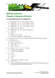
This is an armillary sphere It is a medieval 

scientific instrument that stands about 3 m tall – 

around double the height of the average person. 

It was constructed in Florence around 1590 and 

took almost a decade to complete. It was used to 

chart the movement of the stars and planets. 

Today a simple computer program could do the 

same job with much greater precision. 

1



UNITS AND CONVENTIONS 

Physics is an experimental science dealing largely with measurements. In Physics, the data 

that you collect and the numbers that you work with in problems are not just numbers. They 

are measurements of physical quantities such as mass, time, temperature, etc. 

Fundamental Units 

In 1960, the international authority on units and measures agreed to adopt a standardised 

system known as the International System (SI) of units. There are many different physical 

quantities, but in the SI system, seven are defined as fundamental or basic quantities. They 

are: 

Fundamental Quantity 

length 

mass 

time 

electric current 

temperature 

luminous intensity 

amount of substance 

Unit and Symbol 

metre (m) 

kilogram (kg) 

second (s) 

ampere (A) 

kelvin (K) 

candela (Cd) 

mole (mol) 

In Physics, we will be dealing with the first 5 of these quantities many, many times! 

Derived Units 

Other physical quantities (e.g. speed) can be measured in units that are derived from these 

fundamental units. 

e.g. Speed is defined as: 

speed 

= 

distance 

travelled 

time taken 

The unit for speed is m/s or m s -1 . This is derived from the fundamental units for length and 

time. 

e.g. The kinetic energy of an object is: E k = 1 2 mv2 

The unit for kinetic energy is: kg × (m/s) 2 = kg m 2 / s 2 or kg m 2 s -2 . Again, this is derived in 

terms of fundamental units. This unit of energy is more commonly known as a joule (J). 

e.g. the unit for area is square metres. Area unit = length unit × length unit = m × m = m 2 

Worked Example 

Newton’s 2 nd Law states that a net force applied to a body is equal to the product of its mass 

and acceleration i.e. ΣF = ma 

What is the derived unit for force? 

Unit of force = 

2



Solution: This derived unit (kg m s -2 ) also has a special name. It is called a newton (N). 

Some derived units are shown in the table below. 

Derived Quantity Unit Symbol 

frequency hertz Hz 

force newton N 

energy or work joule J 

power watt W 

electric potential volt V 

resistance ohm Ω 

temperature degree Celsius °C 

Prefixes 

Often you will be measuring quantities that are very big (e.g. the resistance of your body) or 

very small (e.g. the thickness of a hair). When dealing with values such as these, it is 

necessary to use prefixes with the units. Prefixes represent decimal fractions or multiples of 

the original SI unit. 

Prefix Abbreviation Value 

tera T 10 12 

giga G 10 9 

mega M 10 6 

kilo k 10 3 

milli m 10 -3 

micro µ 10 -6 

nano n 10 -9 

pico p 10 -12 

Notice that these power values occur in multiples of three. This is consistent with the 

convention of organising large numbers in groups of three e.g 15,000,000,000. 

Other prefixes that you will encounter are: centi, c, 10 -2 ; hecto, h, 10 2 and deci, d, 10 -1 

Exercises: Complete these statements:- 

a) 6 MW = W 

b) 6,000 kW = W 

c) 500 ms = s 

d) 15,000 km = m 

e) 3 nm = m 

f) 25 GHz = Hz 

g) 5 µm = m 

h) 0.25 ms = s 

3



Standard Form 

When working with big or small numbers, it is often time consuming or clumsy to write the 

number out in full. For example, the speed of light in a vacuum is 300,000,000 m s -1 . The 

convention is to express this in standard form or scientific notation as 3.00×10 8 m s -1 . 

In tests and exams, it is expected that numbers greater than 1000 or less than 0.01 will be 

written in standard form. 

On your calculator, the EXP button is used for writing values in standard form. 

Use your calculator to determine: 3.00×10 8 ×5.0×10 -6 = 

Conversion of Units 

Often you will need to convert from one unit to another. For example, if you measure the 

length and width of your desk in centimetres, but you want to know its area in square metres. 

You will need to convert square centimetres into square metres. This involves working in 2 

dimensions. 

Area 

100 cm 

100 cm 

1 m 2 1 m 3 1 m 2 = 100 cm × 100 cm 

= 10,000 cm 2 

Similarly, if you measure the length, width and thickness of your textbook in millimetres but 

wish to find its volume in cubic metres. This will involve a 3 dimensional conversion from 

cubic centimetres into cubic metres. 

Volume 

100 cm 

100 cm 

1 m 3 = 100cm × 100cm × 100cm 

= 1,000,000 cm 3 

= 1.0×10 6 cm 3 

100 cm 

Exercises: Complete these conversions: 

(a) 1 cm 2 = mm 2 

(f) 1 cm 3 = mm 3 

(e) 1 m 2 = µm 2 (j) 1 mm 3 = m 3 

(b) 1 km 2 = m 2 

(g) 1m 3 = cm 3 

(c) 1 mm 2 = m 2 

(h) 1 µm 3 = m 3 

(d) 1m 2 = mm 2 

(i) 1 m 3 = km 3 

4



WORKSHEET: Units and Conversions 

Remember to express numbers greater than 1000 or less than 0.01 in 

standard form! 

1. Convert these lengths into metres (m): 

a) 25,000,000 µm = 

b) 33 nm = 

c) 360,000 mm = 

2. Convert these areas into square metres (m 2 ): 

a) 1500 cm 2 = 

b) 60,000 µm 2 = 

c) 0.42 km 2 = 

3. Convert these volumes into cubic centimetres (cm 3 ): 

a) 35,000 mm 3 = 

b) 3 m 3 = 

c) 56,000,000 µm 3 = 

4. Convert these current readings into amperes (A): 

a) 370 mA = 

b) 90,000 µA = 

c) 0.03 µA = 

5. Convert these mass measurements: 

a) 44 kg = g 

b) 64,000 mg = g 

c) 70,000,000,000 µg = kg 

6. Express these units in terms of the fundamental SI units. 

Name and Symbol Definition Unit Special Name 

force, F mass×acceleration kg m s -2 newton, N 

momentum, p 

mass×velocity 

work, W force×distance joule, J 

velocity, v 

acceleration, a 

impulse, I 

displacement/time 

velocity/time 

force×time 

charge, Q current×time coulomb, C 

voltage, V 

resistance, R 

work/charge 

voltage/current 

5



MEASUREMENT 

Expressing the Accuracy of a Measurement 

When you obtain a measurement during an experiment or work with measurements when 

solving problems, you need to be mindful of a number of important conventions. 


When you obtain data during an experiment, the accuracy of a measurement will depend on 

the precision of the instrument or meter being used. 

For example, if you use a metre rule to measure the diameter of a ball bearing, you might 

obtain a result of 1.2 cm. However, if you used a micrometer to measure the diameter instead, 

the result might be 1.258 cm. The micrometer is far more precise and gives a much more 

accurate answer. 

The metre rule has given two figures or digits that we know about with some confidence. We 

say that the data (1.2 cm) has 2 significant figures. The data from the micrometer (1.258 cm) 

has allowed us to know the diameter of the ball bearing to 4 significant figures. 

The number of significant figures in a measurement can be found using 4 simple rules: 

• All non-zero figures are significant, e.g. 15.75 kg has 4 significant figures. 

• All zeros in between non-zero digits are also significant, e.g. 2.09 m has 3 sig figs. 

• All zeros that follow a non –zero digit and are to the right of the decimal point are 

significant. 

e.g. 21.40 g has 4 significant figures. 

0.5 mm has 1 significant figure. 

0.100 kg has 3 significant figures. 

• Zeros used for placing very small or very large numbers are not significant. 

e.g. 0.00000031 V has 2 significant figures 

4,550,000,000,000,000 m has 3 significant figures. 

It is often confusing when dealing with whole numbers ending with zero. 

For example; 6,600 mm could have 2, 3 or 4 significant figures. 

To overcome this confusion, it should be written in standard form as: 

6.6×10 3 mm if you wish to show 2 sig figs, or 

6.60×10 3 mm if you wish to show 3 sig figs and so on. 

6



Addition and Subtraction of Measurements 

When adding or subtracting data, the measurements must be rounded off to the least number of 

decimal places that are present in the data. 

e.g. 

13.305 mm 

10.24 mm 

+2.0522 mm 

25.5972 mm 

This must be rounded off to 2 decimal places (25.60 mm) because 10.24 has just 2 decimal places. 

The same applies for subtraction problems. 

Multiplication and Division of Measurements 

When multiplying or dividing data, your answer must be rounded off to the least number of 

significant figures in your data. 

e.g. 0.50 cm × 26.84 cm = 13.42 cm 2 . 

This must be rounded off to 13 cm 2 because 0.50 cm has 

only 2 sig figs. 

2 sig figs 4 sig figs 

The same applies when dividing measurements. 

NB: These rules only apply when working with measurements. For example, if the mass of one 

marble is 26.7 g, then the mass of 5 identical marbles is: 

5×26.7 g = 133.5 = 134 g. The answer still has 3 significant figures. The ‘5’ is not a 

measurement! What are its units?? 

Also take care when using pi! 

TAKE NOTE!! 

You must be mindful of significant figures when writing practical reports and when 

answering test questions. If you have too many or too few significant figures in your data or 

in your answers, you will lose marks!!! 

7



WORKSHEET: SIGNIFICANT FIGURES 

1. The length of an object is measured 3 times using 3 different measuring instruments. 

The results obtained were: a) 92.71 mm b) 93 mm c) 9 cm 

Which result was obtained using a blackboard ruler, a micrometer and a 30 cm ruler? 

2. For each of the measurements recorded below, write down its number of significant figures 

and express it in scientific notation with the correct SI unit. The first example has been 

completed for you. 

Measurement Significant figures Standard Form, SI unit 

(a) 13.05 kg 4 13.05 kg 

(b) 0.0000063 A 

(c) 27 kJ 

(d) 353,000,000 mm 

(e) 0.00607 mm 

(f) 0.250 µA 

(g) 150 kg 

3. How many significant figures are quoted in each of the following measurements? 

a) 783.9 kJ b) 0.035 cm c) 90.24 kg d) 86,400 s e) 0.0060 m f) 6.07×10 7 m 

4. What is the perimeter of a soccer field if its length and width were measured to be 95.82 m 

and 71.836 m respectively? 

5. What is the area (in m 2 ) of the soccer field discussed in Question 4? 

6. Use your 30 cm ruler to measure the length and width of this page. 

length = cm 

width = cm 

Use these results to determine: (a) the perimeter of the page (b) the area of the page 

7. Mary runs 25.3 m in 4.1 s. What was her average speed? 

8




When we take measurements and readings with different analogue instruments, there is 

always a limit to how accurately we can obtain our results. If we use a metre ruler to measure 

the thickness of a 50 c coin, we can gain a result to the nearest millimetre i.e. 2 mm. 

However, if we use a more precise instrument such as a micrometer (which measures to the 

hundredth of a millimetre!), we could say that the thickness is 2.46 mm. If using a digital 

device that is giving a stable reading, there is an uncertainty of ±1 in the last digit. The 

accuracy with which we record all our measurements must reflect the type of device that was 

used to obtain the measurements. We should not record too many decimal places, nor should 

we record too few. 

This measurement would be recorded as 225 g. It is not 

possible to read it more precisely, as say 224.3 g. It would 

also be incorrect to write down 225.00 g. 

This measurement could be 

accurately recorded as 450.75 g. 

Exercise:. 

1. Record each of the analogue measurements below to the appropriate level of precision 

2. What is the uncertainty for these digital readings? 

(a) 16.3 g (b) 52 °C (c) 2.06 mA (d) 0.094 mm 

9



Uncertainties in Single Measurements 

When we take measurements and readings, there is always uncertainty involved. This 

uncertainty is related to the quality of the apparatus and the skill of the experimenter. It is not 

possible to obtain exact values! Most measurements will vary slightly from the actual value. 

The difference between the two is the error or uncertainty. 

NB: an error does not necessarily imply a mistake; just an imprecision!! 

Absolute errors 

The reading taken using the ruler shown above would be recorded as 55.6 cm. However, the 

actual length will in fact be slightly higher or lower than 55.6 cm. Using the ruler, we can 

distinguish between 55.5, 55.6, and 55.7 cm, but is unreasonable to say that the measurement 

is 55.63 cm. This ruler is only accurate to the nearest millimetre. To indicate that the length is 

somewhere between 55.5 and 55.7 cm, we can say that: 

length = 55.6±0.1 cm 

This ±0.1 cm is known as the absolute uncertainty associated with the reading. In general, 

the uncertainty associated with any measured value is taken to be half of the limit of the 

reading of the device, or half of the smallest division of the scale being used. 

The smallest division on the metre ruler above is 0.2 cm, hence the uncertainty is 0.1 cm. 

What absolute uncertainty would apply if you used your ruler? 

According to this convention, the reading on the force meter on the previous page should be 

recorded as 0.3±0.05 N. This reading, however, is not strictly correct. There are some other 

important rules and conventions that must be followed! 

• There must be the SAME NUMBER OF DECIMAL PLACES in both the 

MEASUREMENT and the ABSOLUTE UNCERTAINTY. 

e.g. 55.7±0.1 cm 30.35±0.05 kg 74±2 g 

e.g. 46.1±0.06 mm 85±0.5 kg 43.6±1 mA 

• An absolute uncertainty must only have ONE SIGNIFICANT FIGURE and will often 

need to be rounded off. 

10



For example, if a scale has a smallest division of 0.5 N, the absolute uncertainty will be ±0.25 

N which will need to be rounded off to ±0.3 N. 

If the scale of the instrument is very large, you can use your judgement to determine the 

uncertainty. 

In the example below, half of the smallest division is 0.25 which must be rounded off to 0.3. 

This would give a reading of 4.6±0.3 which suggests that the value could be anywhere 

between 4.3 and 4.9. We can obviously be more precise than that. In this case, the value 

could be recorded as 4.60±0.05. 

Percentage Errors 

An uncertainty could also be expressed as a percentage error. 

percentage 

absolute error 100 

error = 

! 

measurement 1 

0.05 100 

In this example, the percentage error is: % error = ! = 1.1% 

4.60 1 

Percentage errors are usually written with: 

• 1 significant figure when less than 1% 

• 2 significant figures when 1% or greater. 

For example, if you calculate an error to be 0.75%, you should round this off to 0.8%. Also, 

an error of 5.681% needs to be rounded off to 5.7%. 

Percentage errors give a better representation of the accuracy of the measurement than do 

absolute errors. Consider these 2 measurements: 

530±5 s and 10±5 s 

The absolute error is the same in each measurement (±5s) , but this error is far more 

significant in the second case. 

5 100 

The percentage error for the first result is: % error = ! = 0.94% 

. This is very 

530 1 

accurate; less than 1% error. 

In the second measurement, the error is 50%. Perhaps the experimental technique used needs 

to be improved in order to obtain more precise data! 

11



Examples of correct and incorrect error readings are given below. Complete the ones that are 

missing. 

Incorrect Reading Correct Version Incorrect Reading Correct version 

20.876±0.2 s 20.9±0.2 s 7.5±0.62 m/s 

27±0.6 mm 27±1 mm 0.352±0.02 ms 

85.45±0.25 kg 85.5±0.3 kg 59±1.6 m 3 

28.6 K ± 0.87% 28.6 K± 0.9% 8.05 km± 4.71% 

WORKSHEET: UNCERTAINTY EXERCISES 

1. Fix up these incorrect measurements: 

(a) 57±0.5 mm 

(f) 10.4±0.065 mm 

(b) 112.3±1 m/s 

(g) 15±2.5 mA 

(c) 1.6±0.05 mg 

(h) 0.34±0.15 kg 

(d) 64.4±1.8 m 

(i) 27.03±0.1 kg 

(e) 0.085±0.0025 kV 

(j) 45.0±2 m 

2. Determine the percentage uncertainties for your answers in Question 1. 

3. Record the readings on these meters and scales as accurately as is appropriate. Indicate the associated 

uncertainties, being mindful of the conventions that you have just learnt. 

12



Showing Uncertainties on Graphs 

Many experiments in Physics can be analysed using graphs. When drawing graphs, straight 

lines or curves of best fit must be plotted. There should be about the same number of data 

points above and below these lines of best fit. 

There is an uncertainty associated with each point that is plotted on a graph. Error bars are 

used to show this uncertainty. 

E.g. Consider the following data: 

length(cm) 

resistance (Ω) 

14.5±0.5 0.22±0.02 

Let us consider how the data should be shown on the graph. First, we plot the data value 

(14.5 cm, 0.22 Ω). Then we must indicate the uncertainty of this point using error bars. 

For the resistance data, the value could range from a minimum of 0.22 – 0.02 = 0.20 up to a 

maximum of 0.22 + 0.02 = 0.24. We indicate this range by drawing a line between 0.20 and 

0.24 Ω as shown on the graph. This line is called an error bar. 

Similarly, the error bar for length should be drawn between 14.0 and 15.0 cm. 

• It is important to remember that your line of best fit should pass through or touch ALL of 

the error bars that you have drawn. 

• Often, error bars will be too small to be shown on a graph. If this is the case, include a 

statement to that effect underneath the graph. However, the uncertainties must always 

be shown in your tables of results. 

• When doing graphical analysis, it is usually only necessary to show error bars on your 

first graph. 

Worksheet: Error bars! 

13



Advanced Error Analysis 

Sometimes you may wish to use your data to obtain a different physical quantity. For 

example, you have measured the length and width of a classroom as 5.85±0.05 m and 4.2±0.1 

m respectively. Now want to calculate the perimeter and area of the room. You can do this by 

performing a simple calculation. It is also possible to determine the uncertainty for these 

derived quantities. 

Adding and Subtracting Measurements 

The room has: length = 5.85±0.05 m 

width = 4.2±0.1 m 

4.2±0.1 m 

5.85±0.05 m 

To calculate the perimeter value, you will need to perform the following addition: 

5.85 m 

4.2 m 

5.85 m 

+ 4.2 m___ 

20.10 m_ 

Recall that the answer is limited by the least number of decimal places for addition and 

subtraction problems. In this case, that is 1 decimal place. The answer must therefore be 

given as: 

Perimeter = 20.1 m. 

When adding or subtracting 

measurements, the total absolute error 

is found by ADDING the individual 

absolute errors. 

The uncertainty is therefore: 0.1+0.05+0.1+0.05 = 0.30 m. 

Recall that absolute errors can only have 1 significant figure, so the measurement must be 

written as: 

Perimeter = 20.1±0.3 m 

The technique for subtraction is the same i.e the absolute errors are ADDED! This would 

be useful when finding the error associated with the change in a quantity. 

14



Multiplying and Dividing Measurements 

If you wished to calculate the area of the classroom, you would simply multiply the length 

and width measurements. 

4.2±0.1 m 

5.85±0.05 m 

Area = 4.2×5.85 = 24.57 m 2 

Recall that when measurements are multiplied or divided, the answer is limited by the least 

number of significant figures in the measurements. In this example, the least number is two 

(in 4.2 m), so this answer must be written as: 

Area = 25 m 2 

To calculate the absolute error for this value, you must add the percentage errors of the 

measurements. 

% error for length = 0.05 

5.85 " 100 

1 = 0.85% 

% error for width = 0.1 

4.2 "100 1 = 2.4% 

The percentage error for area is:0.85 + 2.4 = 3.25%. This would be rounded off to: 

Area = 25 m 2 ±3.3% 

The absolute error for area is found simply calculating 3.3% of 25 m 2 = ±0.83m 2 . So the 

area value can be stated as: Area = 25 ±0.83 m 2 

However, the absolute error can only have 1 significant figure, so the final result must be 

given as: 

Area = 25 ±1 m 2 

When multiplying or dividing measurements, the individual 

percentage errors must be ADDED to find the total percentage 

error. 

15



ERROR ANALYSIS EXERCISE 

1. Consider the following dimensions of a room in an art gallery. Calculate, giving both 

percentage and absolute errors, the following quantities. 

h = 4.1±0.1 m 

(a) the floor perimeter. 

l = 27.4±0.3 m 

w = 3.45±0.02 m 

(b) perimeter of the large wall. 

(c) the floor area. 

(d) the large wall area. 

(e) the difference between the length and width of the floor. 

(f) the volume of the space. 

16



Uncertainties when taking Repeat Samples 

When performing experiments in class, time constraints usually mean that only one 

measurement is taken for each data point. This measurement is quite unreliable because there 

may have been inaccuracies with the equipment or in the way in which the result was 

obtained for that particular result. As you will be aware, if you repeat the same experiment 4 

or 5 times, you will get 4 or 5 slightly different values. This does not mean that you have 

done something wrong; it simply indicates the random nature of uncertainties. (If your 

results are vastly different, however, you might want to have a look at your experimental 

technique!). 

In order to obtain results that are more reliable, it is necessary to take repeat samples for 

each particular data point and use this to obtain an average value. It is always better, 

although not always possible, to obtain 3, 4 or more results for each value. 

For example, some students are testing the rebound height of a golfball dropped from 1.00 m 

onto a concrete floor. In order to obtain reliable data, they repeat the experiment 7 times. 

Their results were: 

Rebound height (cm) 81 88 84 49 85 84 87 

It is clear that something went wrong with the 4 th result! This outlier can be disregarded. 

81+ 88 + 84 + 85 + 84 + 87 

The average rebound height is : = 84.8 cm 

6 

The data had 2 significant figures, so this answer must be rounded off to 85 cm. 

Note that if you had stopped after taking only one result, it would have given 81 cm. 

To find the absolute error for the average value: 

( highest value ! lowest value) 

absolute error = 

2 

In this example, the absolute error is: 

88 " 81 

= ±3.5 cm 

2 

This must be rounded off to 1 significant figure, i.e.±4, so the average rebound height and 

its absolute error is: 

85±4 cm. 

Remember, absolute errors should be: 

• recorded to 1 significant figure 

• have the same level of precision as the data value 

17



Repeat Samples worksheet 

A group of students took the following measurements of the length, width and depth of a 

swimming pool. 

Depth (m) Width (m) Length (m) 

3.01 8.75 50.03 

3.04 8.70 50.10 

2.98 8.63 50.07 

2.97 8.68 50.01 

3.00 8.71 49.98 

3.02 8.72 49.97 

3.03 8.67 50.00 

(a) Calculate the average depth, width and length of the pool. Include absolute errors with 

your answers. 

(b) Use your answers to determine these quantities. Include both absolute and percentage 

errors with your answers. 

(i) The top surface area of the pool. 

(ii) The volume of the pool. 

(iii) The perimeter of the pool bottom. 

18



HOMEWORK EXERCISE: MARBLES! 

Name: 

In an experiment, Lyn had to measure the time taken for a marble to drop through a tube 

filled with water. She made two marks on the tube; one near the top and one near the bottom. 

She started the stopwatch just as the marble passed the top mark and stopped timing as the 

marble passed the bottom mark. 

She repeated the experiment 5 times. 

Trial number time(s) 

1 3.2 

2 2.7 

3 2.9 

4 3.5 

5 3.3 

water 

Lyn then filled the tube with cooking oil and repeated the experiment. Her results were: 

Trial number time(s) 

1 6.7 

2 6.5 

3 6.7 

4 6.7 

5 6.8 

oil 

1. In which experiment does the data seem to be more accurate? Discuss. 

2. For each of the experiments above, calculate the average time that the marble took to 

travel between the marks. Include the absolute error in your answer. 

3. If the distance between the marks was 1.05±0.01 m, determine the average speed of the 

marble as it fell through each liquid. Include absolute errors and units in your answers. 

19



DATA ANALYSIS 

Experimental Design 

The SCIENTIFIC METHOD is an objective, unbiased and powerful way of investigating 

phenomena. This scientific approach has only been developed over the past few centuries and 

it has led to the explosion in knowledge and technological advances during that time. 

First, observed facts or data are sorted into some logical order. Then a hypothesis or 

explanation is put forward. This hypothesis is used to make predictions that can be tested to 

either support or disprove the hypothesis. From the results of these tests, conclusions can be 

drawn. If enough data has been collected, it may be possible to propose a law that predicts 

future outcomes. A theory (explanation of why the law works) could then be proposed and 

subjected to further testing. 

When designing an experiment to investigate the relationship between two variables, it is 

important that you control the variables in the experiment to ensure that the experiment is 

fair. 

• The variable that you are controlling and making changes to is called the 

INDEPENDENT VARIABLE. 

• The variable that responds to the changes in the independent variable is called the 

DEPENDENT VARIABLE. 

• The factors that remained the same throughout the experiment are called CONTROLLED 

VARIABLES. 

EXAMPLES: For each of these experiments, identify the independent, dependent and what 

could act as controlled variables. 

Experiment 1: Ten seeds were planted in each of 5 pots (A-E) containing Budget Potting 

Mix. The pots were given the following amounts of water each day for 40 days: A: 50 mL, B: 

100 mL, C: 150 mL, D: 200 mL, E: 250 mL. 

Experiment 2: Jenny wanted to see if the colour of food influenced whether kindergarten 

children would choose it for lunch. She put food colouring into 4 identical bowls of mashed 

potato and counted how many children chose each colour. The colours were red, green, 

yellow and blue. 

Experiment 3: James wished to investigate the relationship between the angle of a Hot 

Wheels track and the time that a car takes to travel down the track. He used 1.50 m of track, 

placed it at an angle of 10° to the horizontal and timed how long the toy car took to travel 

down it. He repeated this with angles of 20°, 30°, 40° and 50°. 

20



How to write up a Formal Practical Report! 

The main reason that scientists report on the results of their experiments is so that others can 

read and understand what was done and what the results may tell us. Obviously, for this 

purpose to be achieved, a lot of care needs to taken when writing up experiments and 

communicating your findings. When writing up a practical report, your expression should be 

clear, concise and unambiguous. 

Each formal experiment report that you write should contain the following headings:- 

AIM: Every experiment must have an aim (or aims) otherwise there is no point doing it! 

The aim could be to investigate the nature of the relationship between two (or more) 

variables. This investigation could be qualitative (describe the general nature of the 

relationship) or quantitative (define a precise mathematical relationship). 

You should discuss the variables involved. Identify:- 

the independent variable (the one you were manipulating), 

the dependent variable (the one that changes when the independent variable is changed) and 

controlled variables (things that you have kept unchanged). 

APPARATUS: list the laboratory equipment that was used. It is not necessary to include 

items such as pens and calculators. 

METHOD: This is a description of how you and your partner performed the experiment. 

This should be written in past tense and in the third person (i.e. no names!). 

✘ We recorded the temperature every 10 seconds. 

✓ The temperature was recorded every 10 seconds. 

Explain clearly what you did. Include descriptions of any modifications that you had to make 

or any problems that you encountered. Describe steps that you undertook to ensure that the 

data that you collected was accurate. 

It is important to include a scientific diagram of how the apparatus was set up. 

RESULTS: These are usually placed in tables and graphs. 

Tables should include the names and abbreviated units of the quantities that you measured. 

Record an appropriate number of significant figures in your table. 

Table 1: time for car to travel down ramp at different angles 

Length of ramp = 2.35±0.05 m 

Angle (±0.5º) Time (±0.1 s) 

5.3 6.4 

6.4 5.2 

Underneath the table, explain how you decided on the uncertainty values that you used. 

Include sample calculations with your explanations. 

21



Graphs should include the same information as the tables, but marked on the axes: 

Time(s) 

Graph 1: Time vs Angle for car travelling down ramp 

× 

× 

× 

× 

Angle (º) 

Graphs can be done on computer or by hand. If on computer, show the grid lines. If by hand, 

use pencil and do on graph paper. 

Give your graph a detailed heading. Make sure that the scale is marked along each axis. 

Mark in the main numerical values (not the data points) and make sure that each scale is 

even! Most graphs will start from the origin. 

Mark points as small crosses and show the line of best fit. If this is straight, use a ruler. If it is 

a curved, carefully sketch one smooth curved definite line that travels as close to as many 

points as possible. Don’t play join the dots! 

ANALYSIS: This usually consists of a series of directed questions relating to the data. This 

is the most important part of the report. Make sure that you explain your findings clearly 

giving full responses. 

In the analysis sections of Student Designed Investigations, you should begin by having a 

general discussion of the data. Refer to your tables and graphs. Then try to identify any 

patterns or trends that seem evident. Ensure that your discussion is detailed. 

Can you find the relationship between the variables? You can use graphical analysis to 

establish a quantitative relationship. Make sure that you fully explain the process that you 

have undertaken, showing gradient calculations, etc. 

What do current theories say about the relationship between your variables? Discuss how 

your findings compare with theory. You will be assessed on the depth of your analysis. A full 

and detailed analysis will be rewarded; a brief and superficial analysis will not. 

CONCLUSION: This is a response to the Aim. Briefly state your main findings from doing 

the experiment. If you have found a relationship, state what it is. 

DISCUSSION OF UNCERTAINTIES: In any experiment involving measurements, 

uncertainties will arise. In point form, you should discuss where these uncertainties occurred. 

Don’t explain how you arrived at the actual values again. For example: 

During this experiment, uncertainties occurred for the following reasons: 

As the car was released, it may have been pushed or retarded slightly. 

Stopwatches were used to measure the time taken by the car. Allowing for reaction times, this 

led to an uncertainty in these measurements. 

On some occasions, the car did not travel directly along the ramp, leading to an uncertainty in 

the distance measurements. 

There was an uncertainty associated with drawing a line of best fit. 

22



Doing Graphs and Tables on EXCEL 

Open EXCEL and enter your data in the spreadsheet. Put the x co-ordinate data in column 1 

and the y co-ordinate data in column 2. Include the units that were used in brackets. For 

example, if you wished to plot a speed vs time graph: 

time ( 0.2s) speed ( 0.4 m s -1 ) 

0.0 0.6 

1.0 2.5 

2.0 3.8 

3.0 5.9 

4.0 7.4 

5.0 9.3 

NB: EXCEL cannot do ± signs, so you will need to enter the ±’s by hand after printing out 

the table. 

Producing a Graph 

Highlight the table, including the headings, and then click on the “chart wizard” icon. 

STEP 1: Select x-y scatter (without plotted lines). 

STEP 2: 

Data range: series in: columns. 

STEP 3: Titles – 

Chart title: Graph 1: speed vs time for parachute (You can 

also type your name here) 

Value X axis: time(s) 

Value Y axis: speed (m/s) 

Gridlines – show MAJOR gridlines 

Legend – untick ‘show legend’ 

Data labels: none 

STEP 4: 

Chart location – as new sheet → FINISH 

Plotting a line of best fit 

In physics, we would like you to rule or sketch your own line of best fit so that your 

graphing skills improve! 

For your own purposes, you may wish to use EXCEL to do this: 

In the toolbar, click on CHART – ADD TRENDLINE. 

TYPE: select the line that best matches the data. For straight lines, choose LINEAR. 

OPTIONS: If you want the line to pass through the origin; set intercept = 0 

NB: don’t display the equation on the chart. 

23



Plotting Error Bars 

Click on one of the points on your graph. This should highlight all of the points. 

Click FORMAT – SELECTED DATA SERIES 

To set the error bars, choose the X ERROR BARS and Y ERROR BARS folders. In each 

folder, you should: 

Display: BOTH 

Error amount: FIXED VALUE – insert your absolute error for each variable. 

NB: you cannot enter different uncertainty values for one particular variable. These would 

need to be done manually if required. 

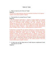
The graph below has uncertainties of ±0.2s for the time values and ±0.4m/s for the speed 

values. 

Graph 1: speed vs time for car rolling down ramp A Einstein 11RCH 

12 

10 

8 

Speed (m/s) 

6 

4 

2 

0 

-1 0 1 2 3 4 5 6 

Time (s) 

Your chart is now ready to PRINT! 

Use this data to do your own table and graph. Hand this in for HOMEWORK!! 

24



Graphical Analysis of Data 

In many experiments, the goal is to determine a relationship between two variables. This can 

be done by plotting a graph with the independent variable on the horizontal-axis and the 

dependent variable on the vertical-axis. 

The shape of the graph can then be used to establish the nature of the relationship! 

Linear graphs 

When you get a linear or straight-line graph, you can easily determine the relationship 

between the variables. Let us consider a simple straight line graph: 

v (m/s) 

v (m/s) 

gradient , m = 

t (s) 

rise 

run 

This graph shows a linear relationship between v and 

t. The mathematical relationship is: v ∝ t. 

The mathematical equation is: v = mt + c 

gradient , m = 

rise 

run 

This graph shows a direct relationship between v 

and t. The mathematical relationship is: v ∝ t. 

The mathematical equation is: v = mt 

t (s) 

The unit associated with the gradient can be determined by finding the ratio of the rise/run 

units. In the examples above, the units of the gradient quantity are: 

riseunit 

rununit 

m s 

= = m s or m s 

s 

2 !2 

Examples: 

1. If the vertical axis is force(N) and the horizontal axis is distance(m), what will the units of 

the gradient be? 

2. If the horizontal axis is time (s) and the vertical axis is distance(m), what will the units of 

the gradient be? 

3. If the vertical axis is degrees (°) and the horizontal axis is degrees (°), what will the units 

of the gradient be? 

25



Non-linear Graphs 

If your graph does not show a direct or linear relationship, it will probably look like one of 

the lines shown below: 

A B C 

D E F 

These are lines obtained for common relationships other than direct or linear relationships. 

All of the above may be expressed mathematically as: y ∝ x n 

and hence by a simple equation: 

y = kx n 

where y is the dependent variable, x is the independent variable, and k and n are both 

constants. 

n is usually one of –2, -1, -½, 0, ½, 1, 2 or 3. The coefficient k has a unit, but n is 

dimensionless! 

Exercise 

1. For each graph shown above, write down: 

the type of relationship that it shows (in words). 

the mathematical relationship that exists between x and y. 

the mathematical equation between x and y. 

2. What is the value of n for: A? B? C? D? E? F? 

3. What is the value of n for a linear relationship? 

26



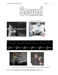
Finding the quantitative relationship! 

If the graph that you plot looks like one of those just discussed, you can determine the correct 

nature of the relationship by plotting additional graphs. 

• First, plot the original data. 

• Second, decide what the relationship could be i.e. it may look like a square relationship. 

• Third, plot a graph of your guess i.e. a vs b 2 . (You will need to calculate b 2 values to do 

this.) 

• Then, if this graph is a straight line, you can work out the equation. 

F 

Plot data and identify relationship. 

parabola ⇒ square relationship F ∝ t 2 

t 

F 

If this graph is linear, you can calculate the 

gradient and work out the equation. 

i.e. F = gradient × t 2 

t 2 

If your first guess was incorrect, i.e. you guessed y ∝ x 3 , your graph of y vs x 3 will not give 

a straight line and you will need to have another go! 

NB: a relationship and hence an equation can only be determined if a straight line graph 

has been obtained. 

It is important that you follow the graphical analysis process and are not influenced by 

your knowledge of what the relationship might be. For example, if you are investigating 

the relationship between light intensity I and distance d, you could find that I ∝ 1/d 2 from 

a text book. As a scientist, however, you must not let this affect the way that you analyse 

the data. You must act as though you do not know the outcome and first plot a graph of I 

vs d. This should be hyperbolic, so you would next plot I vs 1/d. If this is linear, you 

would have to conclude that your relationship was inverse in nature and be prepared to 

discuss why your results differed from the known value. You might find that this graph is 

parabolic and so would plot I vs 1/d 2 . If this graph was linear, you could conclude that 

there was an inverse square relationship between I and d and you would be able to say 

that your findings agreed with the theoretical relationship. 

27



Graphical Analysis Exercises 

1. Beneath each graph, indicate the most likely relationship that exists and state the 

equation expressing this relationship. 

P B L 

(a) (b) (c) 

Q A M 

2. What graph would you plot to check your answer to 1(a)? 

3. What graph would you plot to check your answer to 1(b)? 

4. What graph would you plot to check your answer to 1(c)? 

5. Using graphical analysis, work out the equation that defines the relationship between the 

pairs of variables below. Also indicate the value of k and give its unit. 

(a) (b) (c) 

mass 

(kg) 

acceleration 

(m s -2 ) 

velocity 

(m s -1 ) 

kinetic energy 

(J) 

diameter 

(cm) 

resistance, 

(Ω) 

1.00 98 0.00 0.00 0.60×10 -2 51.3 

2.00 52 1.00 2.05 1.0×10 -2 16.0 

4.00 24.1 2.00 7.90 1.3×10 -2 10.2 

5.00 20.4 3.00 17.6 1.7×10 -2 5.9 

10.0 9.7 4.00 32.5 3.5×10 -2 1.42 

In each case, the first variable is the independent variable. This must be plotted on the 

horizontal axis. 

Show your graphs and calculations on the graph paper following! 

28



mass, 

(kg) 

acceleration, 

(m s -2 ) 

1.00 98 

2.00 52 

4.00 24.1 

5.00 20.4 

10.0 9.7 

29



Answers to Worksheets and Exercises 

velocity 

(m s -1 ) 

kinetic 

energy (J) 

0.00 0.00 

1.00 2.05 

2.00 7.90 

3.00 17.6 

4.00 32.5 

30



diameter, resistance (Ω) 

(cm) 

0.60×10 -2 51.3 

1.0×10 -2 16.0 

1.3×10 -2 10.2 

1.7×10 -2 5.9 

3.5×10 -2 1.42 

31



32



Answers to Exercises 

Prefixes 

(a) 6,000,000 W 

(b) 6,000,000 W 

(c) 0.5 s 

(d) 15,000,000 m 

(e) 0.000000003 m 

(f) 25,000,000,000 Hz 

(g) 0.000005 m 

(h) 0.00025 s 

Conversion of Units 

(a) 100 mm 2 

(b) 1.0×10 6 m 2 

(c) 1.0×10 -6 m 2 

(d) 1.0×10 6 mm 2 

(e) 1.0×10 12 µm 2 

(f) 1.0×10 3 mm 3 

(g) 1.0×10 6 cm 3 

(h) 1.0×10 -18 m 3 

(i) 1.0×10 -9 km 3 

(j) 1.0×10 -9 m 3 

Worksheet: Units and Conversions 

1(a) 25 m 

(b) 3.3×10 -8 m 

(c) 360 m 

2(a) 0.15 m 2 

(b) 6.0×10 -8 m 2 

(c) 4.2×10 5 m 2 

3(a) 35 cm 3 

(b) 3.0×10 6 cm 3 

(c) 5.6×10 -5 cm 3 

4(a) 0.37 A 

(b) 0.09 A 

(c) 3.0×10 -8 A 

5(a) 4.4×10 4 g 

(b) 64 g 

(c) 70 kg 

6. kg m s -1 

N m 

m s -1 

m s -2 

N s 

A s 

J C -1 

V A -1 


1(a) micrometer 

(b) 30 cm ruler 

(c) metre ruler 

2(b) 2, 6.3×10 -6 A 

(c) 2, 

(d) 3, 

(e) 3, 

(f) 3, 

(g) 2 or 3, 

3(a) 4 

(b) 2 

(c) 4 

(d) 3 

(e) 2 

(f) 3 

4. 335.31 m 

5. 6883 m 2 

7. 6.2 m s -1 

2.7×10 4 J 

3.53×10 5 m 

6.07×10 -6 m 

2.50×10 -7 A 

150 kg 


1. 5.4 mm 3 

0.5 N 

360 K 

30°C 

55 cm 

740 g 

0.3 N 

2 (a) ±0.1 g (b) ±1°C (c) ±0.01 mA (d) ±0.001 mm 

Uncertainty Exercises 

1(a) 57±1 cm 

(b) 112±1 m s -1 

(c) 1.6±0.1 mg 

(d) 64±2 m 

(e) 0.085±0.003 kV 

(f) 10.4±0.1 mm 

(g) 15±3 mA 

(h) 0.3±0.2 kg 

(i) 27.0±0.1 kg 

(j) 45±2 m 

2(a) 1.8% 

(b) 0.9% 

(c) 6.3% 

(d) 3.1% 

(e) 3.5% 

(f) 1% 

(g) 20% 

(h) 67% 

(i) 0.4% 

(j) 4.4% 

3(a) 2.6±0.1 

(b) 0.5±0.1 

(c) 1.90±0.01 

(d) 30±1 

(e) 0.017±0.001A 

(f) 110±5V 

(g) 2.7±0.1V 

(h) 25±5mA 

(i) 3.9±0.1V 

33



Error Analysis Exercises 

1(a) 61.7±0.6 m; 61.7 m ±1.0% 

(b) 63.0±0.8 m; 63.0 m ±1.3% 

(c) 94.5 m 2 ±1.7%; 95±2 m 2 

(d) 110 m 2 ±3.5%; 110±4 m 2 

(e) 24.0±0.3 m; 24.0 m ±1.3% 

(f) 390 m 3 ±4.1%; 390±20 m 3 

Repeat samples worksheet 

(a) D = 3.01±0.04 m 

W = 8.69±0.06 m 

L = 50.02±0.07 m 

(b) (i) 435 m 2 ±0.8%; 435±3 m 2 

(ii) 1310 m 3 ± 2.1%; 1310±30 m 3 

(iii) 117.4 ± 0.3 m; 117.4 m ± 0.3% 

Graphical Analysis Exercises 

1(a) square; P = kQ 2 

(b) inverse; B = k/A 

(c) square root; L = k√A 

2. P vs Q 2 

3. B vs 1/A 

4. L vs √M 

5(a) k = 100 kg m s -2 ; a = 100/m 

(b) k = 2.0 J m -2 s 2 ; E K = 2.0 v 2 

(c) k = 0.0018 Ω cm 2 ; R = 0.0018/d 2 

Homework Exercise: Marbles! 

1 The percentage error for oil is much lower. 

The times for oil are more accurate because the 

marble would be moving more slowly making it 

easier to time precisely. 

2 water: 3.1±0.4 s; oil; 6.7±0.2 s 

3 water: 0.34±0.05 m s -1 ; oil: 0.16±0.01 m s -1 

Non-linear Graphs Exercise 

1(a) independent; y is independent of x; no 

equation 

(b) square; y ∝ x 2 ; y = kx 2 

(c) cubic; y ∝ x 3 ; y = kx 3 

(d) square root; y ∝ √x; y = k√x 

(e) inverse; y ∝ 1/x; y = k/x 

(f) inverse square; y ∝ 1/x 2 ; y = k/x 2 

2(a) 0 

(b) 2 

(c) 3 

(d) 0.5 

(e) –1 

(f) –2 

3. one 

34

Units and Conventions Measurement Data Analysis ... - PEGSnet

Create successful ePaper yourself

Delete template?

Save as template?