Introducing the Differentiated All-Pole and One-Zero Gammatone ...

Introducing the Differentiated All-Pole and One-Zero
Gammatone Filter Responses and their Analog VLSI
Log-domain Implementation
A. G. Katsiamis 1 , E. M. Drakakis 2
Department of Bioengineering (The Sir Leon Bagrit Centre)
Imperial College London
London, UK
1. andreas.katsiamis@imperial.ac.uk
2. e.drakakis@imperial.ac.uk
Richard F. Lyon, Fellow, IEEE
Foveon Inc.,
2820 San Tomas Expressway,
Santa Clara CA 95051
dicklyon@acm.org
Abstract—The scope of this paper is to introduce two particular
filter responses which closely resemble tuning curves at
specific set of places on the basilar membrane (BM) of the biological
cochlea. The responses are termed Differentiated All-
Pole Gammatone Filter (DAPGF) and One-Zero Gammatone
Filter (OZGF) and their form suggest their implementation by
means of cascades of N identical two-pole systems, which
makes them excellent candidates for efficient analog VLSI
implementations. The resulting filters can be used in a filterbank
architecture to realize cochlea implants or auditory processors
of increased biorealism. In addition, their simple
parameterization allows the use of conventional automatic gain
control (AGC) schemes to model certain important features of
the biological cochlea (e.g. level-dependent gain) that are observed
physiologically. To illustrate the idea, we present preliminary
simulation results from a 4 th -order OZGF using novel
high dynamic range log-domain biquads in CMOS weak inversion
(CMOS-WI). All circuits were designed in Cadence®
Design Framework, using the commercially available AMS
0.35µm CMOS process. The reported OZGF structure has a
simulated input dynamic range of 114.5dB, while dissipating
3.7µW of static power.
function. In addition, it is not easy to use the parameterization
of the GTF to model level-dependent changes in the
auditory filter.
N −1
The Gamma-distribution: At exp( − bt)
(1.1)
The tone: cos( ω + φ ) (1.2)
N −1
The Gammatone: At exp( − bt) cos( ω t + φ)
(1.3)
r
The parameters order N (integer), ringing frequency ω r
(rad/s), starting phaseφ (rad), and one-sided pole bandwidth
b (rad/s), together with (1.1) - (1.3) complete the description
of the GTF.
r t
I. INTRODUCTION
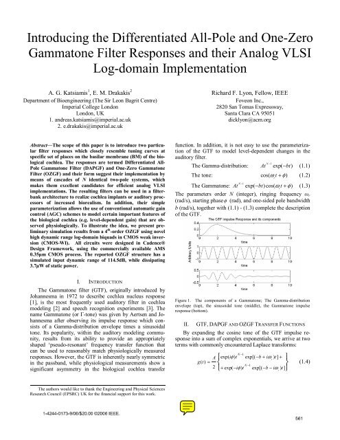
The Gammatone filter (GTF), originally introduced by
Johannesma in 1972 to describe cochlea nucleus response
[1], is the most frequently used auditory filter in cochlea
modeling [2] and speech recognition experiments [3]. The
name Gammatone (or Г-tone) was given by Aertsen and Johannesma
after observing its impulse response which consists
of a Gamma-distribution envelope times a sinusoidal
tone. Its popularity, within the auditory modeling community,
results from its ability to provide an appropriately
shaped ‘pseudo-resonant’ frequency transfer function that
can be used to reasonably match physiologically measured
responses. However, the GTF is inherently nearly symmetric
in the passband, while physiological measurements show a
significant asymmetry in the biological cochlea transfer
Figure 1. The components of a Gammatone; The Gamma-distribution
envelope (top), the sinusoidal tone (middle), the Gammatone impulse
response (bottom).
II. GTF, DAPGF AND OZGF TRANSFER FUNCTIONS
By expanding the cosine tone of the GTF impulse response
into a sum of complex exponentials, we arrive at two
terms with commonly encountered Laplace transforms:
⎧
N −1
A exp( iφ) t exp[( − b+ iω
) t]
+
r
gt () = ⎨
N −1
2 + exp( −iφ) t exp[( −b−iω
) t]
⎩
r
⎫
⎬
⎭
(1.4)
The authors would like to thank the Engineering and Physical Sciences
Research Council (EPSRC) UK for the financial support for this work.

N−1
N
Using the relation t exp( pt) →Γ( N) ( s − p)
, identifying
p with the complex pole location –b + iω r and its conjugate,
we arrive at the Gammatone’s Laplace transform or the GTF
transfer function G(s):
N
AΓ( N)
⎧exp( iφ)[ s−( −b− iω
)] + ⎫
r
⎨
⎬
N
2 ⎩+ exp( −iφ)[ s−( − b+
iω
)]
r ⎭
Gs () =
(1.5)
2 2
N
⎡⎣( s+ b)
+ ω ⎤
r ⎦
Г(N) is the Gamma-function and is defined as Г(N)=(N–1)!,
whereas A can in practice be an arbitrary gain factor. Expressing
b and ω r in terms of the pole-frequency ω o and
quality factor Q and dropping the AΓ(N)/2 gain term without
any loss of generality, we obtain the Q-parameterization of
G(s):
N
⎧ ⎡ ⎛ ωo
2 ⎞⎤ ⎫
exp( iφ) s− − −iω
1− 1 4Q
+
o
⎪
⎢ ⎜
⎟
2Q
⎥ ⎪
⎨
⎣ ⎝ ⎠⎦
N ⎬
⎪ ⎡ ⎛ ωo
2 ⎞⎤
+ exp( −iφ) s− − + iω
1−1 4Q
⎪
o
⎪
⎜
⎟
⎩
⎢
⎣ ⎝ 2Q
⎠⎦
⎥ ⎪⎭
Gs () =
(1.6)
N
⎡ 2 ωo
2⎤
s + s+
ω
⎢
o
⎣ Q
⎥
⎦
The above transfer function may be considered as the addition
of two individual N th -order complex pole terms which
add with constructive or destructive interference. Note that
G(s) may have a zero at s=0 for particular phasesφ of the
GTF. On a dB scale this means that the low-frequency tail
may head towards minus infinity at DC depending on the
particular combination ofφ , N and Q. Moreover, at very
high frequencies the N zeros may cancel out N of the poles
resulting in an ultimate high-frequency roll-off rate of 6N
dB/Oct. Fig.2 illustrates a 4 th -order GTF frequency response
with the phase angleφ varying from 0 to π/2.
Figure 2. The GTF frequency response of order 4 and Q=1 for various
phase angles.
The “spurious” zeros appearing in the numerator of the
GTF transfer function are a limitation when one considers
the implementation of this auditory filter in the analog domain.
That probably explains why all the GTF realizations in
the literature are digital implementations. Good approximations
to the GTF, which keep all its important features but at
the same time can be implemented efficiently in the analog
domain, are the Differentiated All-Pole and One-Zero Gammatone
Filters or DAPGF and OZGF respectively. The
DAPGF is derived by discarding all the zeros of the GTF
apart from one at DC, whereas the OZGF can have a zero
anywhere on the real axis; the resulting transfer functions are
described by (1.7) and (1.8):
Ks
HDAPGF
() s =
(1.7)
2 ωo
2 N
[ s + s+
ωo
]
Q
Ks ( + a)
HOZGF
() s =
(1.8)
2 ωo
2 N
[ s + s+
ωo
]
Q
2N–1
By choosing K to be ω o the H DAPGF (s) can be split into a
product of two transfer functions, namely an All-Pole
Gammatone Filter approximation (APGF) [4] (in this case, a
cascade of N–1 identical lowpass biquads) and an appropriately
scaled bandpass biquad.
2N
−1
ωo
s
HDAPGF
() s =
2 ωo
2 N
[ s + s+
ω
o
]
Q
(1.9)
2N
−2
ωo
ωos
= ×
2 ωo
2 N −1 2 ωo
2
[ s + s+ ωo
] s + s+
ωo
Q
Q
Similarly, the H OZGF (s) can be split into an APGF and an
appropriately scaled lossy bandpass biquad (i.e. a 2-pole, 1-
zero transfer function).
2N
−1
ωo
( s+
a)
HOZGF
() s =
2 ωo
2 N
[ s + s+
ω
o
]
Q
(1.10)
2N
−2
ωo
ωo( s+
a)
= ×
2 ωo
2 N −1 2 ωo
2
[ s + s+ ωo
] s + s+
ωo
Q
Q
The beauty of the transfer functions (1.9) and (1.10), lies
not only in their convenient form towards efficient analog
circuit realizations, but also in their ability to exhibit realistic
asymmetry in the frequency domain, providing a potentially
better match to psychoacoustic data. The DAPGF exhibits
a reasonable bandwidth and centre frequency variation,
while maintaining a linear low-frequency tail only by varying
a single level-dependent parameter (its quality factor, Q).
The OZGF exhibits the exact same characteristics as the
DAPGF, while allowing the variation of the DC level of its
low-frequency tail. To ease circuit realization, it is more
practical to choose the position of the zero to change in accordance
to the quality factor (in other words set α=ω o /Q).
Lastly, it is important to note, that since the DAPGF and
OZGF are essentially cascaded structures, very large gain
variations can be realized while the respective quality factors
are small and vary little.
How do these behaviors relate to the biological cochlea?
The careful observation of Fig.3 will reveal that the actual

frequency response at a particular place on the BM of the
biological cochlea is an asymmetric bandpass response. The
cochlea adapts itself according to the strength of the incoming
input sound. For loud sounds, it becomes passive providing
low (or no) gain in the passband, whereas for weak
sounds it becomes highly selective with the peak gain reaching
60dB or higher. Moreover, the actual peak shifts to the
right (i.e. towards higher frequencies) as the input level decreases;
this shift is accompanied by an increase in spectral
selectivity. This behavior is reflected in both the DAPGF and
OZGF with the additional flexibility of the OZGF to adjust
the DC level of its low-frequency tail.
We have analyzed, characterized and parameterized the
DAPGF and OZGF and obtained graphs which show how
gain, bandwidth, low-side dispersion and roll-off slopes can
be traded-off in terms of Q and the order N. Essentially, we
have provided a set of ‘design curves’ for fitting these responses
to measured physiological data (see Fig.6 for an
indicative example). These results will be published in full
detail elsewhere.
Figure 3. Frequency domain responses obtained from the mammalian
cochlea at a particular position on the BM [5]. Note that the frequency axis
is in linear scale. The responses would look much more selective, if it were
to be plotted in logarithmic scale.
Figure 6. The DAPGF Peak Gain iso-N responses. Observe that for a 4 th -
order DAPGF with a Q of 10, the overall gain is at 80dB (check with
Figs.4, 5 and 11).
III. ANALOG VLSI IMPLEMENTATION
From the preceding discussion, it can be concluded that
the successful implementation of the DAPGF or OZGF lies
in the ability of the engineer to create high performance biquads.
By high performance, we imply high-dynamic-range
and/or low-power, if the system is intended for an implantable
or portable device. In this paper, we present preliminary
simulation results from an OZGF designed in accordance
with the architecture shown in Fig.7.
Figure 4. The DAPGF frequency response of order 4 and with Q ranging
from 1 to 10.
Figure 7. Simplified proposed OZGF channel architecture.
Figure 5. The OZGF frequency response of order 4 and with Q ranging
from 1 to 10. Observe how the filter shape changes from a low peak gain
lowpass shape (Q=1, loud sounds) to a pseudo-resonant bandpass like
shape (Q=10, weak sounds).
The design is comprised by eight Class-A biquads connected
in a pseudo-differential Class-AB arrangement to
increase the dynamic range. The biquads were implemented
in CMOS-WI using the log-domain circuit technique together
with a non-linear-state cross-coupling scheme to ensure
that all internal currents, for the respective Class-A biquads
at each branch, remain strictly positive at all times [6].
The input current conditioner was chosen to be a geometric

mean splitter due to its good frequency response and lower
DC levels, ensuring lower static power consumption and
noise (relative to the harmonic mean splitter). Fig.8 depicts a
simplified circuit schematic of the Class-AB biquad, whereas
the implemented transfer functions are described by (1.11)
and (1.12). Moreover, moving the positioning of the biasing
current I Q from point A to point B, results in the implementation
of a 2-pole, 1-zero transfer function, described by (1.13).
By inspection: ω o =I o /nCU T (where n is the subthreshold
slope parameter and U T is the thermal voltage) and Q= I o /I Q .
I W W
U L
OUT −
LP 2 2
o T
=
=
U L
I I − I
2
IN IN IN
I W W
s
2
( I nCU )
(1.11)
( I nCU )
o T
2
s ( I nCU )
+ +
( I I )
o
Q
( I nCU ) s
( I nCU )
o T
s ( I nCU )
U L
OUT −
BP 1 1
o T
=
=
U L
I I − I
2
IN IN IN
U L
IOUT
W −W
2P1Z
1 1
=
U L
I I − I
IN IN IN
s
=
s
2
+ +
( I I )
o
Q
⎛ I ( )
o
⎞⎡
I nCU ⎤
o T
⎜ ⎟⎢
s + ⎥
⎝ nCU ( )
T
⎠⎣
I I
o Q ⎦
( I nCU )
o T
+ s + ( I nCU )
o T
( I I )
o
Q
o
o
T
T
2
2
(1.12)
(1.13)
Thus, I IN
U
and I IN L (i.e. the inputs to the two branches of the
Class-AB pseudo-differential OZGF) are kept always positive
because of the geometric mean law (1.14).
Figure 9. Simplified circuit topology of the geometric mean splitter. I BIAS
can be set arbitrarily small to reduce the noise.
IV. SIMULATION RESULTS
The circuits were synthesized and simulated using Cadence
® IC Design Framework and the 0.35µm AMS CMOS
process parameters. This section, presents ω o and Q tunability,
dynamic-range and Monte-Carlo results for a 4 th -order
(i.e. an 8 th -order cascaded filter structure) OZGF. The filter
was implemented using PMOS devices, due to their separate
well connections (in the WI region, it is required that V BS =0
to ensure accurate exponential/logarithmic conformity). The
dimensions of the PMOS devices were set to 300µm/1.5µm
in order to extend the WI region to the µA range and reach
sub-millivolt matching. All NMOS devices (used in current
mirrors not shown in Figs.8 and 9) have dimensions
60µm/8µm. Most transistors were in fact cascoded to reduce
V DS variations but we chose not to include them in the schematics
for simplicity and clarity. The power supply and the
capacitors were set to 1.8V and 20pF respectively.
A. Frequency Response
Figs.10 and 11 show ω o and Q tunability of the OZGF
structure (transfer function 1.10). In Fig.10, I o was varied
from 2nA to 20nA, while I Q was set to 2nA (so the Q gradually
changes from 1 to 10). In Fig.11, I o was fixed at 20nA,
while I Q was varied from 2nA to 20nA. Large-signal verification
of the frequency response was also carried out.
Figure 8. Simplified circuit topology of the log-domain pseudodifferential
Class-AB biquad. The feeding (by means of cascoded mirrors)
of the currents W i U (W i L ) to the lower (upper) topology, ensures the true
Class-AB operation of the filter.
The simplified geometric mean splitter circuit is depicted
in Fig.9. From the translinear loop, one can deduce that
U L
2
I I = I (1.14)
In addition,
IN IN BIAS
U L
IN IN IN
I = I − I (1.15)
Figure 10. ω o tunability by means of biasing current I o of the 4 th -order
CMOS-WI log-domain Class-AB OZGF.

frequency response for the chosen device dimensions. Fig.12
shows the peak gain distribution of 200 simulation runs.
µ = 83.712
σ = 15.3583
N = 200
Figure 11. Q tunability by means of biasing current I Q of the 4 th -order
CMOS-WI log-domain Class-AB OZGF.
Figure 12. Monte-Carlo simulation results showing the peak gain
distribution of the 4 th -order CMOS-WI log-domain Class-AB OZGF with a
Q of 10. Out of 200 runs, 156 filters had peak gains ranging from 72 to 82
dB. The theoretically calculated peak value is at 80dB.
B. Linearity, Noise and Power Consumption
The linearity of the whole structure was assessed by performing
single-tone tests and reporting the value of the THD
for various input strengths 1 . The tone’s frequency was set at
the peak of the passband. We report results for two such
tests; one for the low-Q and one for the high-Q response. The
minimum signal that the structure can process is determined
by its input noise floor. The total input-referred noise floor
was determined by integrating within the 3dB bandwidth.
The noise floor value used to determine the input dynamic
range corresponded to that of the high-Q situation, since in
practice the structure will automatically adapt itself (through
an AGC mechanism) to amplify small signals. Table 1 summarizes
the performance of the reported 4 th -order OZGF.
Nominal
Values
TABLE I. OZGF SIMULATED PERFORMANCE
f MAX = 3.069KHz
I o= 20nA; C = 20pF
Q = 1; V DD=1.8V
f MAX = 4.15KHz
I o= 20nA; C = 20pF
Q = 10; V DD=1.8V
Power Consumption 3.67µW 3.728µW
Gain deviation 4.4% 1.13%
Input-Referred Noise 110pA 13.2pA
Linearity THD @ m=350: 4% THD @ m=0.01: 1%
As explained above, the input dynamic range of the system
is defined by the following relation:
m* I (for lowest Q and THD = 4%)
o
DR = (1.16)
noise floor (for highest Q)
From Table 1 and (1.16), the simulated input dynamic range
of the 4 th -order OZGF is found to be 114.5dB.
C. Monte-Carlo
This section presents indicative Monte-Carlo results to
show how process and mismatch variations affect the filter’s
1 The input amplitude was set to m*I o . Thus, the index m indicates
how many times larger or smaller is the input zero-to-peak amplitude
relative to the biasing current I o .
V. CONCLUSIONS
We have presented the DAPGF and OZGF responses
which closely resemble the behavior observed from the biological
cochlea. Their form and simple parameterization
seem to render them ideal candidates for efficient analog
VLSI implementations. The adopted log-domain paradigm
has proven to be an excellent design route towards the implementation
of high-dynamic range frequency shaping networks,
because of the companding nature of the resulting
filter topologies. The designed Class-AB pseudo-differential
log-domain OZGF has a simulated input dynamic range of
114.5dB, while dissipating on average only 3.7µW; these
results compare well with the reported performance of the
healthy mammalian cochleae. A novel AGC mechanism to
automatically adjust the gain of the filter according to the
input strength has already been designed. The whole closedloop
system is currently being fabricated and will be incorporated
in a filterbank architecture to realize superior performance
bionic ear processors for applications such as
speech recognition front-ends, portable health-care devices
and implants for the hearing impaired.
VI.
REFERENCES
[1] Johannesma P.I.M.: ‘The pre-response stimulus ensemble of neuron
in the cochlear nucleus,’ Proceedings of the Symposium of Hearing
Theory, IPO, Eindhoven, The Netherlands, 1972.
[2] Flanagan J.L.: ‘Models for approximating basilar membrane
displacement - Part II. Effects of middle-ear transmission and some
relations between subjective and physiological behaviour,’ Bell Sys.
Tech. J., 1960, 41, pp. 959–1009.
[3] Ishizuka K., Miyazaki N.: ‘Speech feature extraction method
representing periodicity and aperiodicity in sub bands for robust
speech recognition,’ IEEE International conference on Acoustics,
Speech and Signal Processing, Vol.1, pp. 141-144, 17-21 May 2004.
[4] Lyon R.F.: ‘The All-Pole Gammatone Filter and Auditory Models.’
In Forum Acusticum, Antwerp, Belgium, 1996.
[5] Narayan S.S. and Ruggero M.A.: ‘Basilar-membrane mechanics in
the hook region of the chinchilla cochlea,’ In Mechanics of Hearing,
Zao, Singapore, 2000. World Scientific.
[6] D.R. Frey.: ‘A State-Space Formulation for Externally-Linear Class-
AB Dynamical Systems’ IEEE Transactions on Circuits and Systems-
II 46 (3), pp. 306-314, 1999.