LAB 740 - Frequency Response Measurements - Teledyne LeCroy

LeCroy Applications Brief No. L.A.B. 740
Frequency Response Measurements
Derive Frequency Response From Step Response
Filters, amplifiers, and control
systems are usually characterized
by their frequency response
functions. These functions are
usually shown in graphical form
as plots of log amplitude vs. log
frequency called Bode plots.
Oscilloscopes are primarily time
domain measuring instruments.
They represent acquired
waveforms as a time series,
plotting signal amplitude as a
function of time. Utilizing the
mathematical capabilities
available in modern digital
oscilloscopes it is possible to
derive the frequency response
function of a circuit based on the
measured time response to a
step function.
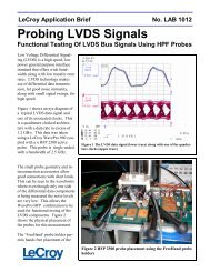
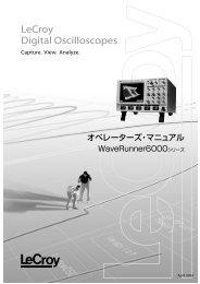
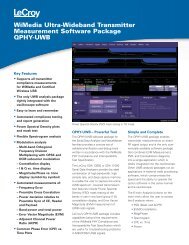
Figure 1 – Transforming the measured step response of a filter
into the frequency response.
An example of this measurement
and analysis is shown in figure 1.
A 1 kHz square wave is applied
to a low pass filter and the output
of the filter is acquired and
displayed in the top trace (Ch 3).
The frequency response function
is the Fourier transform of the
circuits impulse response. The
impulse response can be derived
from the measured step response
by differentiating the step
response. This step is performed
in trace A in figure 1.
To increase the dynamic range of
this measurement and improve
signal/noise ratio the impulse
response is averaged as shown in
trace B.
The Fast Fourier Transform
(FFT) is used to convert the
impulse response into the
frequency response function.
Trace C, not shown applies the
FFT to trace B. Trace D, the
FFT Average function, provides
averaging in the frequency
domain for further improvement
in dynamic range. Note that
number of points used in the
calculations is user selectable. In
this example the transform size
is set to 1000 points yielding a
500 point frequency spectrum.
LeCroy oscilloscopes support
FFT calculations with transform
sizes of up to 4 Mpoints,
dependent on the options
installed.
Trace D, is the frequency
response function shown as a
plot of log amplitude (power
spectrum) vs. linear frequency.
Relative time cursors have been
setup to measure the 3 dB point
of the low pass filter as 33.4
MHz.
This data can be converted into a
classic Bode plot by saving the
frequency spectrum to floppy
disk in spreadsheet format and
plotting it in Log-Log format
using a spreadsheet, such as
Microsoft Excel.

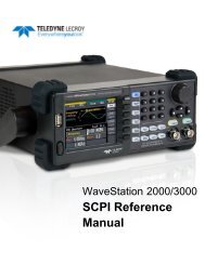
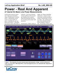
Figure 2 shows the data from
trace D in figure 1, re-plotted
Log – Log format using an Excel
spreadsheet.
LeCroy Applications Brief No. L.A.B. 740
Frequency Response Function
Amplitude dBm
130
120
110
100
90
80
70
60
100000 1000000 10000000 100000000
Frequency (Hz)
Figure 2