Nighttime Cloud Detection Over the Arctic Using AVHRR Data - ARM

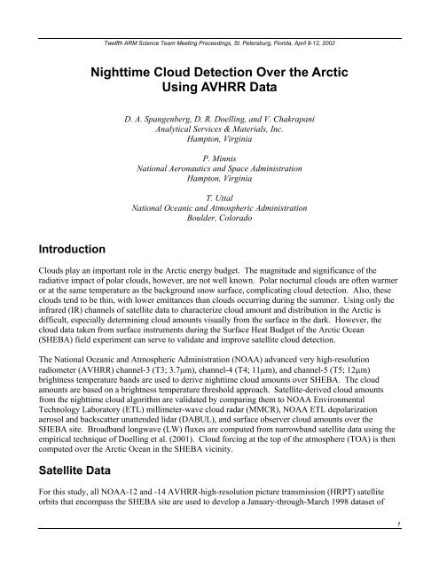
Twelfth ARM Science Team Meeting Proceedings, St. Petersburg, Florida, April 8-12, 2002 

Nighttime Cloud Detection Over the Arctic 

Using AVHRR Data 

D. A. Spangenberg, D. R. Doelling, and V. Chakrapani 

Analytical Services & Materials, Inc. 

Hampton, Virginia 

P. Minnis 

National Aeronautics and Space Administration 

Hampton, Virginia 

T. Uttal 

National Oceanic and Atmospheric Administration 

Boulder, Colorado 

Introduction 

Clouds play an important role in the Arctic energy budget. The magnitude and significance of the 

radiative impact of polar clouds, however, are not well known. Polar nocturnal clouds are often warmer 

or at the same temperature as the background snow surface, complicating cloud detection. Also, these 

clouds tend to be thin, with lower emittances than clouds occurring during the summer. Using only the 

infrared (IR) channels of satellite data to characterize cloud amount and distribution in the Arctic is 

difficult, especially determining cloud amounts visually from the surface in the dark. However, the 

cloud data taken from surface instruments during the Surface Heat Budget of the Arctic Ocean 

(SHEBA) field experiment can serve to validate and improve satellite cloud detection. 

The National Oceanic and Atmospheric Administration (NOAA) advanced very high-resolution 

radiometer (AVHRR) channel-3 (T3; 3.7µm), channel-4 (T4; 11µm), and channel-5 (T5; 12µm) 

brightness temperature bands are used to derive nighttime cloud amounts over SHEBA. The cloud 

amounts are based on a brightness temperature threshold approach. Satellite-derived cloud amounts 

from the nighttime cloud algorithm are validated by comparing them to NOAA Environmental 

Technology Laboratory (ETL) millimeter-wave cloud radar (MMCR), NOAA ETL depolarization 

aerosol and backscatter unattended lidar (DABUL), and surface observer cloud amounts over the 

SHEBA site. Broadband longwave (LW) fluxes are computed from narrowband satellite data using the 

empirical technique of Doelling et al. (2001). Cloud forcing at the top of the atmosphere (TOA) is then 

computed over the Arctic Ocean in the SHEBA vicinity. 

Satellite Data 

For this study, all NOAA-12 and -14 AVHRR-high-resolution picture transmission (HRPT) satellite 

orbits that encompass the SHEBA site are used to develop a January-through-March 1998 dataset of 

1


1,010 images. All hours are sampled by NOAA-12 and -14 except for 6-10 Universal Time Coordinates 

(UTC). The cloud mask algorithm was applied at the 1-km pixel level and the resulting clear-sky and 

cloudy products were averaged within a 25-km radius around the SHEBA site and within 56 × 56-km2 

regional grid boxes. Figure 1 shows the SHEBA ship track and boundary of the regional grid. Satellite 

cloud amounts in this study are defined as the ratio of the cloudy pixels to the total number of pixels. 

Technique 

Figure 1. SHEBA ship track and analysis domain. 

To remove noise inherent in the 3.7-µm band at low temperatures, the images were filtered using a 

parametric Wiener filter developed by Simpson and Yhann (1994). This method works well at night 

when the T3 and T4 images are similar. Because some noise can still be left in the T3-4 images, they 

were smoothed using averages of 16 × 16 pixels. 

Fixed image-independent thresholds were used to derive the satellite cloud mask. The thresholds 

include T3-4, T4-5, T4, the median T4 for the image (T4mid), and the T4 spatial standard deviation 

(T4σ). Because of the calibration differences between NOAA-12 and -14, a different set of thresholds 

was used for each satellite. The Clouds and the Earth’s Radiant Energy System (CERES) nocturnal 

polar cloud mask framework (Trepte et al. 2001) was modified to work with the NOAA-AVHRR 

channels. Figure 2 shows the flowchart of the polar cloud mask algorithm for AVHRR. The algorithm 

2


Figure 2. Flowchart of the polar nighttime cloud mask for AVHRR. 

3


is applied when the solar zenith angle (SZA) is greater than 82°. Clear-sky a priori temperature values 

at the TOA were computed using a correlated k-distribution method (Kratz 1995) incorporating the 

European Centre for Medium-Range Weather Forecasts (ECMWF) profiles. The polar mask first 

performs a series of cloud tests shown in Figure 2. If any of the 12 cloud tests pass, the pixel is 

considered to be cloudy. If the tests fail, then the pixel’s T4-5 value is checked. If that value is below a 

certain threshold, the pixel is classified as clear sky and is subdivided into snow, ocean, or land. 

Because the remaining pixels are difficult to classify during the polar night, weak clear and weak cloud 

categories were defined. For a pixel to be classified as weak clear or weak cloud, the T4-5 value had to 

be above 0.5K for NOAA-12 or 0.3K for NOAA-14. The weak categories often contain surface-based 

aerosol haze, thin cirrus, thin fog, steam fog, or diamond dust. Since the cloudy T4 and T3-4 pixels are 

similar to the underlying surface in the weak categories, thresholding is not always reliable. 

Consequently, the weak categories should be used with caution since confidence in cloud detection is 

fairly low for these cases. 

Note that different tests must be used to pick out warm versus cold clouds in the flowchart (Figure 2). 

The NOAA-12 warm cloud T3-4 tests, which detect a majority of the clouds, require T3-4 to be below 

-1.5K for strong clouds, -0.6K for most clouds, and -0.3K for weak clouds. The corresponding NOAA- 

14 thresholds are 0.7K, 1.9K, and 2.2K, respectively. For warm clouds, T4 must exceed 239K. 

Threshold detection for cold clouds is used if T3-4 is greater than 1.4K for NOAA-12 and 4.0K for 

NOAA-14. For twilight conditions (82° < SZA < 91°), the cloud mask was modified to account for the 

weak visible signature in the T3 image. This was done by increasing the T3-4 thresholds and by adding 

an additional cloud test for relatively high T3-4 values in warm clouds. A special case of twilight tests 

is applied for forward scatter at high satellite view angles. This is necessary because of the very high 

reflectance of T3-4 for this viewing geometry. An example of the cloud mask output, along with 

NOAA-14 T3-4, T4, and T4-5 images for 15:14 UTC, 11 January 1998, are shown in Figure 3. The 

SHEBA site is located in an area of thin warm fog, in the dark region near the center of the T3-4 image. 

The area of high T4 and T3-4 values in the right-hand part of the imagery represents a warm cloud 

system. The clear area in the upper (northern) part of the T3-4 and T4 imagery has values that are 

nearly the same as the cirrus in the lower-right (southern) part of the images. This example illustrates 

the difficulty of detecting cirrus during the polar winter night. 

Results 

Satellite Validation 

The satellite-derived cloud amounts were validated by comparing them with NOAA ETL cloud radar 

amounts over SHEBA for the months of January through March 1998. The DABUL system was used to 

detect thin, low-lying fog or thin cirrus clouds that are not always observed in the MMCR (Intrieri et al. 

2002). DABUL data were only available for January and March 1998. SHEBA 6-hourly surface 

observer cloud amounts were also compared to the cloud radar and were used as a basis for the satellite 

and radar comparisons. The satellite cloud amounts were computed for a 25-km radius around the 

SHEBA ship. Radar cloud amounts are 20-minute time averages of processed 10-second cloud boundary 

data centered at the satellite times. Lidar cloud amounts are the averages of the two 10-minute 

intervals of processed cloud layer data centered at the satellite times. 

4


Figure 3. NOAA-14 satellite image valid at January 11, 1998, 15:14 UTC showing mixed clouds. The 

SHEBA location is denoted by the “S” in the polar mask. 

Monthly statistics of satellite and radar cloud coverage, including means and root-mean-square (rms) 

errors, are shown in Table 1. The statistics were broken down into three radar reflectance (ref) 

categories representing strong cloud signals (ref >= -20 dBZ), weak signals (-50 dBZ < ref < -20 dBZ), 

and clear sky (ref


Table 1. SHEBA ship monthly cloud amount statistics for the radar and satellite. (a) January, 

(b) February, and (c) March 1998 period. 

(a) 

(b) 

(c) 

Radar Reflectance Radar% Sat + % RMS% #Radii 

(dbz) 

ref >= -20 100 94.3 17.2 66 

-50 < ref < -20 85.9 74.4 44.7 44 

ref


Table 2. SHEBA ship cloud amount statistics for the cloud radar and surface observer. 

(a) January, (b) February, and (c) March 1998 period. 

(a) 

(b) 

(c) 

Radar Reflectance 

(dbz) Radar% Obs% RMS% #Obs 

ref >= -20 100 86.8 34.1 36 

-50 < ref < -20 95.2 43.3 69.3 15 

ref


Figure 4. SHEBA domain cloud amounts and temperatures on the regional grid for January-March 

1998. 

indicating that warm clouds are most common during the long winter night over the Arctic Ocean. 

February had the lowest clear-sky temperatures, with typical values around 238K. Table 3 shows a 

comparison between monthly mean cloud, weak cloud, and weak clear amounts for January through 

March 1998. Both clear-sky and cloud temperatures are shown. The total cloud percentage column 

shows the cloud cover for all cloud categories combined. Nighttime cloud cover over the western Arctic 

Ocean is at a minimum of 37% during February and at a maximum of 72% in March. In all 3 months, 

the sum of the weak amounts ranges from 24% to 34% with the weak clear exceeding the weak cloud 

areas. Because of the relatively high amount of weak clear ranging from 14% to 25 %, it is likely that 

the total cloud amounts should be somewhat higher due to cloud contamination within the weak clear 

category. The blue numerals in Table 3 under the weak categories are for percentages relative to the 

total cloud or clear amounts. These numbers show the relative dominance of the weak categories in the 

8


polar mask. Weak clouds account for as much as 24% of all clouds during February. Weak clear ranges 

up to 50% of all clear areas in March. The mean cloud temperature followed the same trend as the 

clear-sky background with the mean cloud temperature exceeding the clear-sky values by 3-4K for all 

three months. 

Table 3. SHEBA domain cloud statistics from the polar cloud mask for January-March 1998. Blue 

numbers in parenthesis are for percent of the total cloud or clear amounts. 

Month # Images 

Total 

Cloud% 

Weak 

Cloud% 

Weak 

Clear% T4 Clear (K) 

T4 Cloud 

(K) 

Jan 350 50.8 10.1 (19.9) 13.7 (27.8) 240.0 243.9 

Feb 312 36.5 8.9 (24.4) 24.6 (38.7) 238.8 241.7 

Mar 285 72.1 11.0 (15.3) 14.0 (50.2) 243.8 246.5 

For the broadband flux results, the AVHRR narrowband IR fluxes were converted into broadband LW 

fluxes using the method outlined in Doelling et al. (2001). Figure 5 shows the winter and spring 

regression fits used to obtain the January-through-March 1998 broadband LW fluxes. Earth Radiation 

Budget Experiment (ERBE) and NOAA-9 AVHRR data from 1986 were matched to obtain the 

regression fits. The different lines are for constant values of column-weighted relative humidity (RH) 

above the radiating surface. The broadband LW flux M lw is computed from the equation 

M lw = a0 + a1*M ir – a2*M ir 2 – a3*Mir*ln(RH), 

where M ir is the narrowband IR flux and a0, a1, a2, and a3 are the coefficients of the regression fit. M lw 

was computed using both the winter and spring regression fits, with the resulting values time 

interpolated to the appropriate month of 1998. LW cloud forcing is defined as 

LWCRF = M lwclr - M lw , 

where M lwclr is the clear-sky LW flux and M lw is the total-sky LW flux. Typical outgoing LW flux 

values range from 165-180W/m 2 in clear-sky regions, with slightly more energy being lost for the totalsky 

case. This leads to a net loss of energy of about 2-6 W/m 2 at TOA due to clouds (negative 

LWCRF). Although wintertime Arctic clouds are primarily warmer than the surface and increase the 

underlying surface temperature, the overall effect on the earth-atmosphere system is a loss of energy at 

TOA. Domain averages of TOA LWCRF, along with the LW fluxes, are shown in Table 4. February 

1998, the month with minimum cloudiness, has the weakest cloud-forcing signal of -2.4 W/m 2 . March 

1998 has the most pronounced loss of energy at TOA, -4.1 W/m 2 . This corresponds to the month of 

maximum cloudiness. 

Table 4. SHEBA domain broadband LW flux statistics for January-March 1998. 

Month Clear LWF (W/m 2 ) Total LWF (W/m 2 ) LWCRF (W/m 2 ) 

Jan 170.1 174.0 -3.9 

Feb 167.6 170.0 -2.4 

Mar 175.4 179.5 -4.1 

9


(a) 

(b) 

Figure 5. Regression fit over the Arctic between AVHRR NOAA-9 narrowband IR flux and ERBE 

broadband LW flux data. (a) November-January 1986 and (b) February-April 1986 period. 

10


SHEBA Ship Results 

To determine how frequently clouds were actually detected in the MMCR data within the weak clear 

and weak cloud categories, the radar cloud amounts were compared to their satellite counterparts when 

the satellite cloud mask yielded large amounts of the weak cloud or weak clear category at the SHEBA 

site. For 18 cases when the polar mask had weak cloud amounts greater than 85%, the MMCR mean 

cloud amount was 72.2%. For 78 cases when the polar mask’s weak clear category was above 85%, the 

radar reported clear skies 61.3% of the time. Further attempts to adjust the thresholds failed to close the 

gap between the satellite polar mask and the ground-based data. In both the weak clear and weak cloud 

areas, T4-5 values are high. This is a signature of relatively high moisture content, which mainly 

occurred in the boundary layer for this study. High moisture content, coupled with strong temperature 

inversions, will help support the formation and maintenance of diamond dust, diffuse ground fog, or 

haze. These phenomena can be invisible to the radar and lidar, but detected as weak cloud in the 

satellite polar mask. Much of the discrepancy between the weak clear amount from the polar mask and 

the ground-based clear-sky amount arises where the radar reflectance is less than -10 dBZ and very little 

signature of the cloud exists in the imagery. Typically, this is the case for thin or scattered cirrus. Also, 

some mixed cloud scenes where cirrus overlays a warm cloud below can be missed as weak cloud in the 

polar mask. 

The monthly mean values of the satellite cloud amount, T4, LW flux, and LWCRF were computed for 

the area within a 25-km radius surrounding the SHEBA ship. For March 1998, 35% of the images were 

not used because they were taken during the daytime. Table 5 shows that cloud coverage is at a 

minimum of 39% in February, with values up to 77% in March. This is the same trend observed in the 

cloud coverage over the regional grid. The clear-sky temperatures are consistently lower than the cloud 

temperatures by 3-4K, leading to a negative cloud forcing of -3 to -4 W/m 2 . These values are similar to 

the regional grid averages, suggesting the SHEBA ship was in an area representative of the rest of the 

western Arctic Ocean. The weak categories have a smaller temperature difference than their 

counterparts, leading to a dampened LW cloud forcing if only the weak clear and weak cloud areas are 

considered. 

Table 5. SHEBA ship cloud amount, cloud temperature, and cloud forcing statistics from the polar 

cloud mask for January-March 1998. 

Month # Images Cloud% 

T4 Clear 

(K) 

T4 Cloud 

(K) 

Clear LWF 

(W/m 2 ) 

Total LWF 

(W/m 2 ) 

LWCRF 

(W/m 2 ) 

Jan 327 46.8 240.2 244.3 170.8 174.1 -3.4 

Feb 292 38.9 239.2 242.9 168.7 172.1 -3.4 

Mar 211 77.0 244.8 247.1 177.3 181.3 -4.0 

Summary and Future Work 

An automated NOAA-AVHRR cloud detection algorithm was developed for polar regions during the 

nighttime. Cloud thresholds used in this study were developed using January-March 1998 satellite data 

over the Arctic Ocean surrounding the SHEBA ship. However, they should be applicable to other 

months or regions of the Arctic with minimal or no adjustment. The satellite-derived cloud amounts 

11


agreed well with radar cloud amounts at the SHEBA site for either high radar reflectances or clear-sky 

radar times. The rms errors between the satellite polar cloud mask and cloud radar results were between 

4% and 25% for these cases. The rms errors for low-reflectivity radar clouds were much higher, both 

for the satellite and surface observer. Since the cloud lidar failed to capture all of the radar returns with 

reflectances less than -20 dBZ, some of the error is likely due to radar clutter. Overall, the polar mask 

performed much better than the surface observers, who usually underestimated nighttime cloud 

coverage. Over the Arctic in winter, the clouds are primarily warmer than the cold background snow 

surface. The coverage increased from 37% in February to 72% in March 1998. The clouds acted to 

cool the earth-atmosphere system with a 2 to 4 W/m 2 loss of energy at the TOA. 

The cloud mask algorithm will be applied to NOAA-AVHRR data taken over the Atmospheric 

Radiation Measurement (ARM) Program - North Slope of Alaska site during 2000 and 2001. The 

CERES polar cloud mask will be applied to the corresponding TERRA-MODIS data. Additional 

satellite-derived cloud products, including estimates of optical depth and cloud height will be available 

for both day and night overpasses. Cloud and radiation products can be found on the web page, 

http://www-pm.larc.nasa.gov. 

Corresponding Author 

Douglas Spangenberg, d.a.spangenberg@larc.nasa.gov, (757) 827-4647 

Acknowledgments 

This research was supported by the Environmental Sciences Division of the U.S. Department of Energy 

Interagency Agreement DE-AI02-97ER62341 under the Atmospheric Radiation Measurement Program. 

References 

Doelling, D. R., P. Minnis, D. A. Spangenberg, V. Chakrapani, A. Mahesh, F. P. J. Valero, and S. Pope, 

2001: Cloud radiative forcing at the top of the atmosphere during FIRE ACE derived from AVHRR 

data. J. Geophys. Res., 106, 15,279-15,296. 

Intrieri, J. M., M. D. Shupe, T. Uttal, and B. J. McCarty, 2002: An annual cycle of Arctic cloud 

characteristics observed by radar and lidar at SHEBA. J. Geophys. Res., in press. 

Kratz, D. P., 1995: The correlated-k distribution technique as applied to the AVHRR channels. 

J. Quant. Spectrosc. Radiative Transfer, 53, 501-517. 

Schneider, G., P. Paluzzi, and J. Oliver, 1989: Systematic error in the synoptic sky cover record of the 

South Pole. J. of Climate, 2, 295-302. 

Simpson, J. J., and S. R. Yhann, 1994: Reduction of noise in AVHRR channel-3 data with minimum 

distortion. IEEE Trans. Geosci. and Remote Sens., 32, 315-328. 

12


Trepte, Q., R. F. Arduini, Y. Chen, S. Sun-Mack, P. Minnis, D. A. Spangenberg, and D. R. Doelling, 

2001: Development of a daytime polar cloud mask using theoretical models of near-infrared 

bi-directional reflectance for ARM and CERES. Proc. AMS 6 th Conf. on Polar Meteorology and 

Oceanography, May 14-18, 2001, 242-245, San Diego, California. 

Young, D. F., P. Minnis, G. G. Gibson, D. R. Doelling, and T. Wong, 1998: Temporal interpolation 

methods for the Clouds and the Earth’s Radiant Energy System (CERES) Experiment. J. Appl. 

Meteorol., 37, 572-590. 

13

Nighttime Cloud Detection Over the Arctic Using AVHRR Data - ARM

Create successful ePaper yourself

Delete template?

Save as template?