Dynamic Economic Load Dispatch of Thermal Power System Using ...
Dynamic Economic Load Dispatch of Thermal Power System Using ...
Dynamic Economic Load Dispatch of Thermal Power System Using ...

You also want an ePaper? Increase the reach of your titles
YUMPU automatically turns print PDFs into web optimized ePapers that Google loves.
IRACST – Engineering Science and Technology: An International Journal (ESTIJ), ISSN: 2250-3498,<br />
Vol.3, No.2, April 2013<br />
<strong>Dynamic</strong> <strong>Economic</strong> <strong>Load</strong> <strong>Dispatch</strong> <strong>of</strong> <strong>Thermal</strong> <strong>Power</strong><br />
<strong>System</strong> <strong>Using</strong> Genetic Algorithm<br />
W. M. Mansour<br />
Pr<strong>of</strong>essor <strong>of</strong> Electrical <strong>Power</strong> <strong>System</strong>s<br />
Shoubra Faculty <strong>of</strong> Engineering, Benha University<br />
Cairo, Egypt<br />
M. M. Salama<br />
Pr<strong>of</strong>essor <strong>of</strong> Electrical <strong>Power</strong> <strong>System</strong>s<br />
Shoubra Faculty <strong>of</strong> Engineering, Benha University<br />
Cairo, Egypt<br />
S. M. Abdelmaksoud<br />
Assistant Pr<strong>of</strong>essor <strong>of</strong> Electrical Engineering<br />
Shoubra Faculty <strong>of</strong> Engineering, Benha University<br />
Cairo, Egypt<br />
H. A. Henry<br />
Demonstrator <strong>of</strong> Electrical Engineering<br />
Shoubra Faculty <strong>of</strong> Engineering, Benha University<br />
Cairo, Egypt<br />
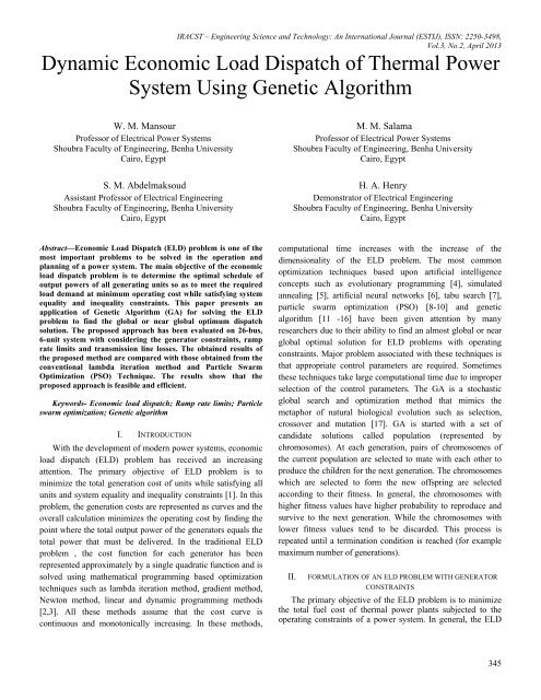
Abstract—<strong>Economic</strong> <strong>Load</strong> <strong>Dispatch</strong> (ELD) problem is one <strong>of</strong> the<br />
most important problems to be solved in the operation and<br />
planning <strong>of</strong> a power system. The main objective <strong>of</strong> the economic<br />
load dispatch problem is to determine the optimal schedule <strong>of</strong><br />
output powers <strong>of</strong> all generating units so as to meet the required<br />
load demand at minimum operating cost while satisfying system<br />
equality and inequality constraints. This paper presents an<br />
application <strong>of</strong> Genetic Algorithm (GA) for solving the ELD<br />
problem to find the global or near global optimum dispatch<br />
solution. The proposed approach has been evaluated on 26-bus,<br />
6-unit system with considering the generator constraints, ramp<br />
rate limits and transmission line losses. The obtained results <strong>of</strong><br />
the proposed method are compared with those obtained from the<br />
conventional lambda iteration method and Particle Swarm<br />
Optimization (PSO) Technique. The results show that the<br />
proposed approach is feasible and efficient.<br />
Keywords- <strong>Economic</strong> load dispatch; Ramp rate limits; Particle<br />
swarm optimization; Genetic algorithm<br />
I. INTRODUCTION<br />
With the development <strong>of</strong> modern power systems, economic<br />
load dispatch (ELD) problem has received an increasing<br />
attention. The primary objective <strong>of</strong> ELD problem is to<br />
minimize the total generation cost <strong>of</strong> units while satisfying all<br />
units and system equality and inequality constraints [1]. In this<br />
problem, the generation costs are represented as curves and the<br />
overall calculation minimizes the operating cost by finding the<br />
point where the total output power <strong>of</strong> the generators equals the<br />
total power that must be delivered. In the traditional ELD<br />
problem , the cost function for each generator has been<br />
represented approximately by a single quadratic function and is<br />
solved using mathematical programming based optimization<br />
techniques such as lambda iteration method, gradient method,<br />
Newton method, linear and dynamic programming methods<br />
[2,3]. All these methods assume that the cost curve is<br />
continuous and monotonically increasing. In these methods,<br />
computational time increases with the increase <strong>of</strong> the<br />
dimensionality <strong>of</strong> the ELD problem. The most common<br />
optimization techniques based upon artificial intelligence<br />
concepts such as evolutionary programming [4], simulated<br />
annealing [5], artificial neural networks [6], tabu search [7],<br />
particle swarm optimization (PSO) [8-10] and genetic<br />
algorithm [11 -16] have been given attention by many<br />
researchers due to their ability to find an almost global or near<br />
global optimal solution for ELD problems with operating<br />
constraints. Major problem associated with these techniques is<br />
that appropriate control parameters are required. Sometimes<br />
these techniques take large computational time due to improper<br />
selection <strong>of</strong> the control parameters. The GA is a stochastic<br />
global search and optimization method that mimics the<br />
metaphor <strong>of</strong> natural biological evolution such as selection,<br />
crossover and mutation [17]. GA is started with a set <strong>of</strong><br />
candidate solutions called population (represented by<br />
chromosomes). At each generation, pairs <strong>of</strong> chromosomes <strong>of</strong><br />
the current population are selected to mate with each other to<br />
produce the children for the next generation. The chromosomes<br />
which are selected to form the new <strong>of</strong>fspring are selected<br />
according to their fitness. In general, the chromosomes with<br />
higher fitness values have higher probability to reproduce and<br />
survive to the next generation. While the chromosomes with<br />
lower fitness values tend to be discarded. This process is<br />
repeated until a termination condition is reached (for example<br />
maximum number <strong>of</strong> generations).<br />
II.<br />
FORMULATION OF AN ELD PROBLEM WITH GENERATOR<br />
CONSTRAINTS<br />
The primary objective <strong>of</strong> the ELD problem is to minimize<br />
the total fuel cost <strong>of</strong> thermal power plants subjected to the<br />
operating constraints <strong>of</strong> a power system. In general, the ELD<br />
345
IRACST – Engineering Science and Technology: An International Journal (ESTIJ), ISSN: 2250-3498,<br />
Vol.3, No.2, April 2013<br />
problem can be formulated mathematically as a constrained 1) As Generation Increases:<br />
optimization problem with an objective function <strong>of</strong> the form:<br />
F<br />
n<br />
T Fi Pi<br />
i = 1<br />
= ∑ ( )<br />
(1)<br />
Where FT<br />
is the total fuel cost <strong>of</strong> the system ($/hr), n is the<br />
total number <strong>of</strong> generating units and Fi( Pi)<br />
is the operating<br />
fuel cost <strong>of</strong> generating unit I ($/hr). Generally, the fuel cost<br />
function <strong>of</strong> the generating unit is expressed as a quadratic<br />
function as given in (2).<br />
2<br />
Fi( Pi)<br />
= aP i i + bP i i + ci<br />
(2)<br />
Where Pi<br />
is the real output power <strong>of</strong> unit i (MW), ai,<br />
bi<br />
and<br />
ci<br />
are the cost coefficients <strong>of</strong> generating unit i. The<br />
minimization <strong>of</strong> the ELD problem is subjected to the following<br />
constraints:<br />
A. Real <strong>Power</strong> Balance Constraint<br />
For power balance, an equality constraint should be<br />
satisfied. The total generated power should be equal to the total<br />
load demand plus the total line losses. The active power<br />
balance is given by:<br />
n<br />
∑ Pi = PD + PL<br />
(3)<br />
i = 1<br />
Where, PD<br />
is the total load demand (MW), PL<br />
represents<br />
the total line losses (MW). The total transmission line loss is<br />
assumed as a quadratic function <strong>of</strong> output powers <strong>of</strong> the<br />
generator units [18] that can be approximated in the form:<br />
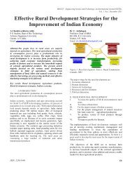
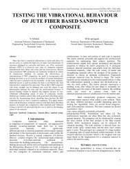
Pi ( t) − Pi ( t − 1) ≤ URi<br />
(6)<br />
2) As Generation Decreases:<br />
Pi ( t − 1) − Pi ( t)<br />
≤ DRi<br />
(7)<br />
Therefore the generator power limit constraints can be<br />
modified as:<br />
max( Pi,min , Pi( t −1) −DRi) ≤Pi( t) ≤ min( Pi,max , Pi( t −1)<br />
+ URi)<br />
(8)<br />
From equation (8), the limits <strong>of</strong> minimum and maximum<br />
output powers <strong>of</strong> generating units are modified as:<br />
Pi min, ramp = max( Pi min , Pi ( t − 1) − DR i)<br />
(9)<br />
Pi max, ramp = min( Pi max , Pi ( t − 1) + UR i)<br />
(10)<br />
Where Pi ( t ) is the output power <strong>of</strong> generating unit i (MW) in<br />
the time interval (t), Pi ( t − 1) is the output power <strong>of</strong> generating<br />
unit i (MW) in the previous time interval (t-1), URi<br />
is the up<br />
ramp limit <strong>of</strong> generating unit i (MW/time-period) and DRi<br />
is<br />
the down ramp limit <strong>of</strong> generating unit i (MW/time-period).<br />
The ramp rate limits <strong>of</strong> the generating units with all possible<br />
cases are shown in Figure 1.<br />
n n<br />
L = iΒ<br />
ij j<br />
i = 1 j = 1<br />
P ∑∑ P P<br />
(4)<br />
Where Βij is the transmission loss coefficient matrix,<br />
Pi<br />
and<br />
th th<br />
Pj<br />
are the power generation <strong>of</strong> i and j units.<br />
B. Generator <strong>Power</strong> Limit Constraint<br />
The generation output power <strong>of</strong> each unit should lie<br />
between minimum and maximum limits. The inequality<br />
constraint for each generator can be expresses as:<br />
Pi ,min ≤Pi ≤P i ,max<br />
(5)<br />
Where Pi<br />
,minand Pi<br />
,maxare the minimum and maximum<br />
power outputs <strong>of</strong> generator i (MW), respectively. The<br />
maximum output power <strong>of</strong> generator is limited by thermal<br />
consideration and minimum power generation is limited by the<br />
flame instability <strong>of</strong> a boiler.<br />
C. Ramp Rate Limit Constraint<br />
The generator constraints due to ramp rate limits <strong>of</strong><br />
generating units are given as:<br />
Figure 1. Ramp rate limits <strong>of</strong> the generating units<br />
III. OVERVIEW OF PARTICLE SWARM OPTIMIZATION (PSO)<br />
Particle swarm optimization (PSO) is a population based<br />
stochastic optimization technique, inspired by social behavior<br />
<strong>of</strong> bird flocking or fish schooling. The PSO algorithm searches<br />
in parallel using a group <strong>of</strong> random particles. Each particle in a<br />
swarm corresponds to a candidate solution to the problem.<br />
Particles in a swarm approach to the optimum solution through<br />
its present velocity, its previous experience and the experience<br />
<strong>of</strong> its neighbors. In every generation, each particle in a swarm<br />
is updated by two best values. The first one is the best solution<br />
(best fitness) it has achieved so far. This value is called Pbest .<br />
Another best value that is tracked by the particle swarm<br />
optimizer is the best value, obtained so far by any particle in<br />
the population. This best value is a global best and called<br />
gbest . Each particle moves its position in the search space and<br />
updates its velocity according to its own flying experience and<br />
neighbor's flying experience. After finding the two best values,<br />
the particle update its velocity according to equation (11).<br />
k + 1<br />
= × k + 1 × 1 × k<br />
( − k<br />
) + 2 × 2 × k<br />
( − k<br />
Vi ω Vi C R Pbest i Pi C R gbest Pi<br />
) (11)<br />
346
IRACST – Engineering Science and Technology: An International Journal (ESTIJ), ISSN: 2250-3498,<br />
Vol.3, No.2, April 2013<br />
k<br />
k<br />
Where V i is the velocity <strong>of</strong> particle i at iteration k, Pi<br />
is Step 7: The position <strong>of</strong> each particle is modified using<br />
the position <strong>of</strong> particle i at iteration k, ω is the inertia weight equation (13).<br />
factor, C 1 and C 2 are the acceleration coefficients, R 1 and R 2<br />
Step 8: Go to step 9 if the stopping criteria is satisfied,<br />
k<br />
are positive random numbers between 0 and 1, Pbesti<br />
is the usually a sufficiently good fitness or a maximum number <strong>of</strong><br />
k<br />
best position <strong>of</strong> particle i at iteration k and gbest is the best iterations. Otherwise go to step 3.<br />
position <strong>of</strong> the group at iteration k.<br />
Step 9: The particle that generate the latest gbest is the<br />
The constants C 1 and C 2 represent the weighting <strong>of</strong> the optimal generation power <strong>of</strong> each unit with the minimum total<br />
stochastic acceleration terms that pull each particle toward cost <strong>of</strong> generation.<br />
Pbest and gbest positions. Low values allow particles to roam<br />
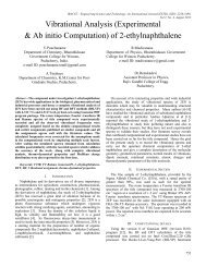
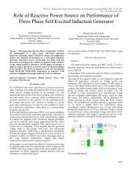
The procedure <strong>of</strong> particle swarm optimization technique<br />
far from the target regions, while high values result in abrupt can be summarized in the flow chart shown in Figure 2.<br />
movement toward, or past, target regions. Hence, the<br />
acceleration constants were <strong>of</strong>ten set to be 2.0 according to past<br />
experiences. Suitable selection <strong>of</strong> inertia weight in equation<br />
(11) provides a balance between local and global searches.<br />
A low value <strong>of</strong> inertia weight implies a local search, while a<br />
high value leads to global search. As originally developed, the<br />
inertia weight factor <strong>of</strong>ten decreases <strong>of</strong>ten is decreased linearly<br />
from about 0.9 to 0.4 during a run. It was proposed in [19]. In<br />
general, the inertia weight ω is set according to equation (12)<br />
ω max−ω<br />
min<br />
ω = ω max− × Iter<br />
(12)<br />
Iter max<br />
Where ω min and ω max are the minimum and maximum<br />
value <strong>of</strong> inertia weight factor, Iter max corresponds to the<br />
maximum iteration number and Iter is the current iteration<br />
number.<br />
The current position (searching point in the solution space)<br />
can be modified by equation (13).<br />
+ 1 + 1<br />
Pi k = Pi k + V i<br />
k<br />
(13)<br />
IV. IMPLEMENTATION OF PSO FOR SOLVING ELD PROBLEM<br />
The step by step procedure <strong>of</strong> the PSO technique for<br />
solving ELD problem is as follows:<br />
Step 1: Select the parameters <strong>of</strong> PSO such as population<br />
size (N), acceleration constants ( C 1 and C 2 ), minimum and<br />
maximum value <strong>of</strong> inertia weight factor ( ω min andω max ).<br />
Step 2: Initialize a population <strong>of</strong> particles with random<br />
positions and velocities. These initial particles must be feasible<br />
candidate solutions that satisfy the practical operation<br />
constraints.<br />
Step 3: Evaluate the fitness value <strong>of</strong> each particle in the<br />
population using the objective function given in equation (2).<br />
Step 4: Compare each particle's fitness with the particles<br />
Pbest . If the current value is better than Pbest , then set<br />
Pbest equal to the current value.<br />
Step 5: Compare the fitness with the population overall<br />
previous best. If the current value is better than gbest , then set<br />
gbest equal to the current value.<br />
Step 6: Update the velocity <strong>of</strong> each particle according to<br />
equation (11).<br />
Figure 2. Flow chart <strong>of</strong> PSO technique<br />
V. GENETIC ALGORITHM (GA)<br />
The GA is a method for solving optimization problems that<br />
is based on natural selection, the process that drives biological<br />
evolution. The general scheme <strong>of</strong> GA is initialized with a<br />
population <strong>of</strong> candidate solutions (called chromosomes). Each<br />
chromosome is evaluated and given a value which corresponds<br />
to a fitness level in problem domain. At each generation, the<br />
GA selects chromosomes from the current population based on<br />
their fitness level to produce <strong>of</strong>fspring. The chromosomes with<br />
higher fitness levels have higher probability to become parents<br />
for the next generation, while the chromosomes with lower<br />
fitness levels to be discarded. After the selection process, the<br />
crossover operator is applied to parent chromosomes to<br />
347
produce new <strong>of</strong>fspring chromosomes that inherent information<br />
from both sides <strong>of</strong> parents by combining partial sets <strong>of</strong> genes<br />
from them. The chromosomes or children resulting from the<br />
crossover operator will now be subjected to the mutation<br />
operator in final step to form the new generation. Over<br />
successive generations, the population evolves toward an<br />
optimal solution. The features <strong>of</strong> GA are different from other<br />
traditional methods <strong>of</strong> optimization in the following respects<br />
[20]:<br />
• GA does not require derivative information or other<br />
auxiliary knowledge.<br />
• GA work with a coding <strong>of</strong> parameters instead <strong>of</strong> the<br />
parameters themselves. For simplicity, binary coded is<br />
used in this paper.<br />
• GA search from a population <strong>of</strong> points in parallel, not<br />
a single point.<br />
• GA use probabilistic transition rules, not deterministic<br />
rules.<br />
A. Genetic Algorithm Operators<br />
At each generation, GA uses three operators to create the<br />
new population from the previous population:<br />
1) Selection or Reproduction:<br />
Selection operator is usually the first operator applied on<br />
the population. The chromosomes are selected based on the<br />
Darwin's evolution theory <strong>of</strong> survival <strong>of</strong> the fittest. The<br />
chromosomes are selected from the population to produce<br />
<strong>of</strong>fspring based on their values. The chromosomes with higher<br />
fitness values are more likely to contributing <strong>of</strong>fspring and are<br />
simply copied on into the next population. The commonly used<br />
reproduction operator is the proportionate reproduction<br />
operator. The i th string in the population is selected with a<br />
probability proportional to Fi<br />
where, Fi<br />
is the fitness value for<br />
that string. The probability <strong>of</strong> selecting the i th string is:<br />
Pr<br />
(14)<br />
Where n is the population size, the commonly used<br />
selection operator is the roulette-wheel selection method. Since<br />
the circumference <strong>of</strong> the wheel is marked according to the<br />
string fitness, the roulette-wheel mechanism is expected to<br />
make Fi<br />
/ F avg copies <strong>of</strong> the i th string in the mating pool. The<br />
average fitness <strong>of</strong> the population is:<br />
F<br />
avg<br />
i<br />
=<br />
=<br />
n<br />
∑<br />
i = 1<br />
n<br />
n<br />
∑<br />
F<br />
j = 1<br />
Fi<br />
i<br />
F j<br />
(15)<br />
2) Crossover or Recombination:<br />
The basic operator for producing new chromosomes in the<br />
GA is that <strong>of</strong> crossover. The crossover produce new<br />
chromosomes have some parts <strong>of</strong> both parent chromosomes.<br />
The simplest form <strong>of</strong> crossover is that <strong>of</strong> single point crossover.<br />
In single point crossover, two chromosomes strings are selected<br />
IRACST – Engineering Science and Technology: An International Journal (ESTIJ), ISSN: 2250-3498,<br />
Vol.3, No.2, April 2013<br />
randomly from the mating pool. Next, the crossover site is<br />
selected randomly along the string length and the binary digits<br />
are swapped between the two strings at crossover site.<br />
3) Mutation:<br />
The mutation is the last operator in GA. It prevents the<br />
premature stopping <strong>of</strong> the algorithm in a local solution. This<br />
operator randomly flips or alters one or more bits at randomly<br />
selected locations in a chromosome from 0 to 1 or vice versa.<br />
B. Parameters <strong>of</strong> GA<br />
The performance <strong>of</strong> GA depends on choice <strong>of</strong> GA<br />
parameters such as:<br />
1) Population Size (N):<br />
The population size affects the efficiency and performance<br />
<strong>of</strong> the algorithm. Higher population size increases its diversity<br />
and reduces the chances <strong>of</strong> premature converge to a local<br />
optimum, but the time for the population to converge to the<br />
optimal regions in the search space will also increase. On the<br />
other hand, small population size may result in a poor<br />
performance from the algorithm. This is due to the process not<br />
covering the entire problem space. A good population size is<br />
about 20-30, however sometimes sizes 50-100 are reported as<br />
best.<br />
2) Crossover Rate:<br />
The crossover rate is the parameter that affect the rate at<br />
which the process <strong>of</strong> cross over is applied. This rate generally<br />
should be high, about 80-95%.<br />
3) Mutation Rate:<br />
It is a secondary search operator which increases the<br />
diversity <strong>of</strong> the population. Low mutation rate helps to prevent<br />
any bit position from getting trapped at a single value, whereas<br />
high mutation rate can result in essentially random search. This<br />
rate should be very low.<br />
C. Termination <strong>of</strong> the GA<br />
The generational process is repeated until a termination<br />
condition has been satisfied. The common terminating<br />
conditions are: fixed number <strong>of</strong> generations reached, a best<br />
solution is not changed after a set number <strong>of</strong> iterations, or a<br />
cost that is lower than an acceptable minimum.<br />
VI. GA APPLIED TO ELD PROBLEM<br />
The step by step algorithm <strong>of</strong> the proposed method is<br />
explained as follow:<br />
Step 1: Read the system input data, namely fuel cost curve<br />
coefficients, power generation limits, ramp rate limits <strong>of</strong> all<br />
generators, power demands and transmission loss coefficients.<br />
Step 2: Select GA parameters such as population size,<br />
length <strong>of</strong> string, probability <strong>of</strong> crossover, probability <strong>of</strong><br />
mutation and maximum number <strong>of</strong> generations.<br />
Step 3: Generate randomly a population <strong>of</strong> binary string.<br />
Step 4: The generated string is converted in feasible range<br />
by using equation (16):<br />
348
P − P<br />
P P P<br />
2 −1<br />
i max i min<br />
gi = i min + ( ). m( i )<br />
L<br />
Where: L is the string length and Pm( i)<br />
is the decimal value<br />
<strong>of</strong> i th generating unit in the string.<br />
Step 5: Calculate the fitness value for each string in the<br />
population.<br />
Step 6: The chromosomes with lower cost function are<br />
selected to become parents for the next generation.<br />
Step 7: Perform the crossover operator to parent<br />
chromosomes to create new <strong>of</strong>fspring chromosomes.<br />
Step 8: The mutation operator is applied to the new<br />
<strong>of</strong>fspring resulting from the crossover operation to form the<br />
new generation.<br />
Step 9: If the number <strong>of</strong> iterations reaches the maximum,<br />
then go to step 10. Otherwise, go to step 5.<br />
Step 10: The string that generates the minimum total<br />
generation cost is the solution <strong>of</strong> the problem.<br />
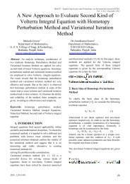
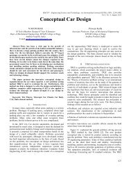
The procedure <strong>of</strong> Genetic Algorithm (GA) can be<br />
summarized in the flow chart shown in Figure 3.<br />
IRACST – Engineering Science and Technology: An International Journal (ESTIJ), ISSN: 2250-3498,<br />
Vol.3, No.2, April 2013<br />
losses [21]. The results obtained from the proposed method<br />
(16) will be compared with the outcomes obtained from the<br />
conventional lambda iteration method and PSO method in<br />
terms <strong>of</strong> the solution quality and computation efficiency. The<br />
fuel cost data and ramp rate limits <strong>of</strong> the six thermal generating<br />
units were given in Table I. The load demand for 24 hours is<br />
given in Table II. B-loss coefficients <strong>of</strong> six units system is<br />
given in Equation (17). Table III gives the optimal scheduling<br />
<strong>of</strong> all generating units, power loss and total fuel cost for 24<br />
hours by using PSO technique. Table IV gives the optimal<br />
scheduling <strong>of</strong> all generating units, power loss and total fuel cost<br />
for 24 hours by using Genetic Algorithm and Table V shows<br />
the total fuel cost comparison between lambda iteration<br />
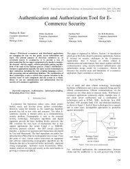
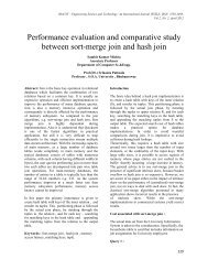
method, PSO method and GA method. Figures (4- 9) show the<br />
relation between fuel cost <strong>of</strong> each unit and 24 hours by the<br />
lambda iteration method, PSO method and GA method.<br />
Some parameters must be assigned for the use <strong>of</strong> GA to<br />
solve the ELD problems as follows:<br />
• Population size = 20<br />
• Maximum number <strong>of</strong> generations = 100<br />
• Crossover probability = 0.8<br />
• Mutation probability = 0.05<br />
And the parameters used in PSO technique to solve the<br />
ELD problem as follows:<br />
• Population size = 20<br />
• Maximum number <strong>of</strong> iterations = 100<br />
• Acceleration constants C 1 = 2.0 and C 2 = 2.0<br />
• Inertia weight parameters ω max = 0.9 and ω min = 0.4<br />
TABLE I.<br />
FUEL COST COEFFICIENTS AND RAMP RATE LIMITS OF SIX<br />
THERMAL UNITS SYSTEM<br />
Unit<br />
a i<br />
($/MW 2 )<br />
b i<br />
($/MW)<br />
c i<br />
($)<br />
P i, min<br />
(MW)<br />
P i, max<br />
(MW)<br />
UR i<br />
(MW/H)<br />
DR i<br />
(MW/H)<br />
1 0.0070 7.0 240 100 500 80 120<br />
2 0.0095 10.0 200 50 200 50 90<br />
3 0.0090 8.5 220 80 300 65 100<br />
4 0.0090 11.0 200 50 150 50 90<br />
5 0.0080 10.5 220 50 200 50 90<br />
6 0.0075 12 190 50 120 50 90<br />
TABLE II.<br />
LOAD DEMAND FOR 24 HOURS OF SIX UNITS SYSTEM<br />
Time<br />
<strong>Load</strong><br />
Time<br />
<strong>Load</strong><br />
Time<br />
<strong>Load</strong><br />
Time<br />
<strong>Load</strong><br />
Figure 3. Flow chart <strong>of</strong> Genetic Algorithm<br />
(H)<br />
(MW)<br />
(H)<br />
(MW)<br />
(H)<br />
(MW)<br />
(H)<br />
(MW)<br />
VII. CASE STUDY AND SIMULATION RESULTS<br />
To verify the effectiveness <strong>of</strong> the proposed algorithm, a six<br />
unit thermal power generating plant was tested. The proposed<br />
algorithm has been implemented in MATLAB language. The<br />
proposed algorithm is applied to 26 buses, 6 generating units<br />
with generator constraints, ramp rate limits and transmission<br />
1 955 7 989 13 1190 19 1159<br />
2 942 8 1023 14 1251 20 1092<br />
3 935 9 1126 15 1263 21 1023<br />
4 930 10 1150 16 1250 22 984<br />
5 935 11 1201 17 1221 23 975<br />
6 963 12 1235 18 1202 24 960<br />
349
B<br />
ij<br />
=<br />
⎡<br />
⎢<br />
1.7 1.2 0.7 - 0.1 - 0.5 - 0.2 ⎤<br />
⎥<br />
⎢<br />
⎢<br />
1.2 1.4 0.9 0.1 - 0.6 - 0.1<br />
⎥<br />
⎥<br />
⎢<br />
⎥<br />
− 3 ⎢ 0.7 0.9 3.1 0.0 - 1.0 - 0.6 ⎥<br />
10 ⎢<br />
⎥<br />
⎢ - 0.1 0.1 0.0 0.24 - 0.6 - 0.8 ⎥<br />
⎢<br />
⎢ - 0.5 - 0.6 - 0.1 - 0.6 12.9<br />
⎥<br />
- 0.2 ⎥<br />
⎢<br />
⎥<br />
⎢⎣<br />
- 0.2 - 0.1 - 0.6 - 0.8 - 0.2 15.0⎥⎦<br />
IRACST – Engineering Science and Technology: An International Journal (ESTIJ), ISSN: 2250-3498,<br />
Vol.3, No.2, April 2013<br />
TABLE V. TOTAL FUEL COST COMPARISON BETWEEN PROPOSED GA<br />
(17)<br />
METHOD, LAMBDA ITERATION METHOD AND PSO METHOD OF 6-UNITS SYSTEM<br />
Method Total Fuel Cost ($)<br />
Lambda iteration method 313045.50<br />
Particle Swarm Optimization (PSO) 313041.40<br />
TABLE III.<br />
OUTPUT POWERS, POWER LOSSES AND TOTAL FUEL COST FOR<br />
24 HR. BY PSO METHOD OF 6-UNITS SYSTEM<br />
Genetic Algorithm (GA) 313040.90<br />
P 1 P 2 P 3 P 4 P 5 P 6 Loss Fuel cost<br />
Hr.<br />
(MW) (MW) (MW) (MW) (MW) (MW) (MW) ($)<br />
1 381.5 120.8 210.4 86.5 112.1 50.0 6.53 11410.86<br />
2 375.6 118.3 208.2 84.9 111.2 50.0 6.35 11248.5<br />
3 372.1 116.8 207.0 84.5 110.6 50.0 6.25 11161.44<br />
4 369.6 115.8 206.1 84.3 110.2 50.0 6.17 11099.41<br />
5 372.1 116.8 207.0 84.5 110.6 50.0 6.25 11161.44<br />
6 384.9 122.2 211.6 87.7 113.0 50.0 6.64 11511.17<br />
7 394.9 126.2 215.8 92.0 116.8 50.0 7.00 11838.94<br />
8 399.0 133.7 222.1 96.2 122.7 56.4 7.38 12270.52<br />
9 420.7 145.6 239.2 114.8 140.7 73.2 8.57 13599.88<br />
10 427.7 148.1 243.1 118.8 143.3 77.7 8.85 13914.45<br />
11 443.1 154.9 247.8 127.5 151.0 85.9 9.50 14588.85<br />
12 452.3 160.5 251.5 133.1 155.4 91.9 9.95 15042.84<br />
13 439.1 153.2 246.5 125.5 150.2 84.4 9.37 14442.65<br />
14 456.1 162.7 254.3 136.3 157.9 93.6 10.18 15257.49<br />
15 458.8 164.5 255.7 138.9 159.2 95.9 10.32 15419.10<br />
16 455.6 162.5 254.1 136.2 157.9 93.6 10.16 15244.01<br />
17 447.6 158.8 250.4 129.9 153.7 90.0 9.78 14855.29<br />
18 443.5 155.0 248.0 127.6 151.1 86.0 9.97 14602.16<br />
19 430.7 149.6 244.1 120.3 144.2 78.8 8.15 14032.85<br />
20 414.3 141.9 233.4 109.2 133.8 67.2 8.38 13157.51<br />
21 399.0 133.7 222.1 96.2 122.7 56.4 7.38 12270.52<br />
22 393.7 125.3 214.9 90.9 115.9 50.0 6.94 11775.78<br />
23 390.2 124.3 213.6 89.0 114.3 50.0 6.82 11662.16<br />
24 383.5 121.5 211.0 87.4 112.9 50.0 6.60 11473.52<br />
Total Fuel Cost ($) 313041.40<br />
F1 ($/hr)<br />
5000<br />
4800<br />
4600<br />
4400<br />
4200<br />
4000<br />
3800<br />
3600<br />
Figure 4.<br />
F2 ($/hr)<br />
2 4 6 8 10 12 14 16 18 20 22 24<br />
Time (24hr)<br />
2300<br />
2200<br />
2100<br />
2000<br />
1900<br />
1800<br />
Lagrangian method<br />
Genetic Algorithm<br />
PSO method<br />
Fuel cost <strong>of</strong> unit 1 versus 24 hr by the three used method<br />
Lagrangian method<br />
Genetic Algorithm<br />
PSO method<br />
TABLE IV.<br />
Hr.<br />
P 1<br />
(MW)<br />
OUTPUT POWERS, POWER LOSSES AND TOTAL FUEL COST FOR<br />
24 HR. BY GA OF 6-UNITS SYSTEM<br />
P 2<br />
(MW)<br />
P 3<br />
(MW)<br />
P 4<br />
(MW)<br />
P 5<br />
(MW)<br />
P 6<br />
(MW)<br />
Loss<br />
(MW)<br />
Fuel cost<br />
($)<br />
1700<br />
1600<br />
1500<br />
1400<br />
2 4 6 8 10 12 14 16 18 20 22 24<br />
Time (24hr)<br />
1 378.4 118.4 210.7 85.4 118.4 50.0 6.58 11411.42<br />
2 373.2 116.0 207.8 84.7 116.4 50.0 6.38 11249.19<br />
3 371.0 114.8 206.1 83.7 115.3 50.0 6.28 11162.06<br />
4 369.3 113.8 205.1 82.9 114.8 50.0 6.21 11099.99<br />
5 371.0 114.8 206.1 83.7 115.3 50.0 6.28 11162.06<br />
6 381.3 119.8 212.1 86.5 119.7 50.0 6.69 11511.66<br />
7 388.9 125.0 217.1 90.8 123.9 50.0 7.06 11838.99<br />
8 395.8 132.8 222.0 97.7 126.3 55.5 7.38 12270.42<br />
9 422.5 147.3 239.5 114.3 138.0 72.7 8.57 13599.96<br />
10 427.1 153.0 243.5 118.8 140.0 76.2 8.86 13914.33<br />
11 438.9 161.9 252.0 128.5 145.8 83.1 9.51 14588.41<br />
12 446.2 166.8 257.8 134.6 150.4 89.0 9.95 15042.04<br />
13 436.9 160.1 250.1 126.2 144.2 81.5 9.37 14442.43<br />
14 450.2 169.5 260.1 136.7 152.7 91.7 10.18 15256.81<br />
15 452.5 171.9 261.6 139.6 154.2 93.2 10.33 15418.34<br />
16 450.0 169.4 259.9 136.5 152.6 91.5 10.16 15243.36<br />
17 443.0 164.9 255.7 131.9 148.2 86.7 9.76 14854.86<br />
18 439.1 162.1 252.2 128.7 145.9 83.2 9.52 14601.71<br />
19 428.9 154.9 244.5 120.8 141.1 77.4 8.96 14032.65<br />
20 411.9 142.0 236.1 108.4 135.3 66.2 8.20 13157.46<br />
21 395.8 132.8 222.0 97.7 126.3 55.5 7.38 12270.42<br />
22 387.9 124.1 215.9 89.8 123.0 50.0 6.99 11775.86<br />
23 385.4 122.1 214.6 88.1 121.5 50.0 6.87 11662.42<br />
24 380.3 119.0 211.7 86.2 119.2 50.0 6.65 11474.06<br />
Total Fuel Cost ($) 313040.90<br />
Figure 5. Fuel cost <strong>of</strong> unit 2 versus 24 hr by the three used method<br />
F3 ($/hr)<br />
3100<br />
3000<br />
2900<br />
2800<br />
2700<br />
2600<br />
2500<br />
2400<br />
2300<br />
Lagrangian method<br />
Genetic Algorithm<br />
PSO method<br />
2 4 6 8 10 12 14 16 18 20 22 24<br />
Time (24hr)<br />
Figure 6. Fuel cost <strong>of</strong> unit 3 versus 24 hr by the three used method<br />
350
F4 ($/hr)<br />
2000<br />
1900<br />
1800<br />
1700<br />
1600<br />
1500<br />
1400<br />
1300<br />
1200<br />
1100<br />
Lagrangian method<br />
Genetic Algorithm<br />
PSO method<br />
2 4 6 8 10 12 14 16 18 20 22 24<br />
Time (24hr)<br />
Figure 7. Fuel cost <strong>of</strong> unit 4 versus 24 hr by the three used method<br />
2200<br />
2100<br />
2000<br />
1900<br />
Lagrangian method<br />
Genetic Algorithm<br />
PSO method<br />
IRACST – Engineering Science and Technology: An International Journal (ESTIJ), ISSN: 2250-3498,<br />
Vol.3, No.2, April 2013<br />
When the Lambda iteration method is used to solve this<br />
system, it has been observed that the minimum cost curve<br />
converges within the range <strong>of</strong> 1500 - 2000 iterations while in<br />
genetic algorithm and particle swarm optimization technique<br />
the cost curve converge within the range <strong>of</strong> 30-50 iterations.<br />
So the computational time <strong>of</strong> the proposed algorithm is much<br />
less than the Lambda iteration method.<br />
VIII. CONCLUSIONS<br />
In this paper, genetic algorithm (GA) is used to solve the<br />
ELD problem. The proposed algorithm has been successfully<br />
implemented for solving the ELD problem <strong>of</strong> a power system<br />
consists <strong>of</strong> 6 units with different constraints such as real power<br />
balance, generator power limits and ramp rate limits. From the<br />
tabulated results, it is clear that the total fuel cost obtained by<br />
GA is comparatively less compared to other methods. GA<br />
approach gives high quality solutions with fast convergence<br />
characteristic compared to the lambda iteration method. The<br />
lambda iteration method is also applicable, but it can converge<br />
to the minimum generation cost after so many iterations. So,<br />
the computational time <strong>of</strong> the lambda iteration method is much<br />
greater than the proposed algorithm. Simulation results<br />
demonstrate that the proposed method is powerful and practical<br />
tool for obtaining global minimum or near global minimum <strong>of</strong><br />
total fuel cost.<br />
F5 ($/hr)<br />
1800<br />
1700<br />
1600<br />
1500<br />
1400<br />
2 4 6 8 10 12 14 16 18 20 22 24<br />
Time (24hr)<br />
Figure 8. Fuel cost <strong>of</strong> unit 5 versus 24 hr by the three used method<br />
F6 ($/hr)<br />
1500<br />
1400<br />
1300<br />
1200<br />
1100<br />
1000<br />
900<br />
800<br />
Lagrangian method<br />
Genetic Algorithm<br />
PSO method<br />
2 4 6 8 10 12 14 16 18 20 22 24<br />
Time (24hr)<br />
Figure 9. Fuel cost <strong>of</strong> unit 6 versus 24 hr by the three used method<br />
REFERENCES<br />
[1] A .J. Wood and B.F. Wollenberg, “<strong>Power</strong> generation, operation, and<br />
control,” John Wiley and Sons., New York, 1984.<br />
[2] Salama, M., M., “<strong>Economic</strong> control for generation in thermal power<br />
system,” Energy Conversion and Management, 40, 1999, pp. 669-681.<br />
[3] IEEE Committee Report, “Present practices in the economic operation <strong>of</strong><br />
power systems,” IEEE Trans. <strong>Power</strong> Appa. Syst., PAS-90, 1971, pp.<br />
1768-1775.<br />
[4] N. Sinha, R. Chakrabarti and P. K. Chattopadhyay, “Evolutionary<br />
programming techniques for economic load dispatch,” IEEE Evol.<br />
Comput. 7, February (1), 2003, pp. 83-94.<br />
[5] K. P. Wong and C. C. Fung, “Simulated annealing based economic<br />
dispatch problem,” IEEE Proc.-C, vol. 140, no. 6, 1993, pp.509-515.<br />
[6] J. Nanda, A. Sachan, L. Pradhan M.L. Kothari, A. Koteswara Rao,<br />
“Application <strong>of</strong> artificial neural network to economic load dispatch,”<br />
IEEE Trans. <strong>Power</strong> <strong>System</strong>s, vol. 22, 1997.<br />
[7] W. M. Lin, F. S. Cheng and M. T. Tsay, “An improved tabu search for<br />
economic dispatch with multiple minima,” IEEE Trans. <strong>Power</strong> Syst., 17<br />
(February (1)) (2002), pp. 108-112.<br />
[8] Z. L. Gaing, “Constrained dynamic economic dispatch solution using<br />
particle swarm optimization,” IEEE <strong>Power</strong> Engineering Society General<br />
Meeting, 2004, pp. 153-158.<br />
[9] J. B. Park, K. S. Lee, J. R. Shin and K. Y. Lee, “A particle swarm<br />
optimization for economic dispatch with non smooth cost functions,”<br />
IEEE Trans. <strong>Power</strong> Syst, 20, February (1), 2005, pp. 34-42.<br />
[10] D. N. Jeyakumar, T. Jayabarathi and T. Raghunathan, “Particle swarm<br />
optimization for various types <strong>of</strong> economic dispatch problems,” Elec.<br />
<strong>Power</strong> Energy Syst, 28, 2006, pp. 36-42.<br />
[11] D. C. Walters and G. B. Sheble, “Genetic algorithm solution <strong>of</strong><br />
economic dispatch with valve point loading,” IEEE Trans. <strong>Power</strong> Syst.,<br />
8 August (3), 1993, pp. 1325-1332.<br />
[12] J. Tippayachai, W. Ongsakul and I. Ngamroo, “Parallel micro genetic<br />
algorithm for constrained economic dispatch,” IEEE Trans. <strong>Power</strong> Syst.,<br />
17 August (3), 2003, PP. 790-797.<br />
[13] A. Bakirtzis, etal. “Genetic algorithm solution to the economic dispatch<br />
problem,” IEE Proc. Generation, Transmission and Distribution,<br />
vol.141, no.4, July 1994, pp. 377-382.<br />
351
IRACST – Engineering Science and Technology: An International Journal (ESTIJ), ISSN: 2250-3498,<br />
Vol.3, No.2, April 2013<br />
[14] G. B. Sheble and K. Brittig, “Refined genetic algorithm-economic [18] J. A. Momoh, M. E. El-Hawary and R. Adapa, “A review <strong>of</strong> selected<br />
dispatch example,” IEEE Trans. on <strong>Power</strong> <strong>System</strong>s, vol. 10 ,no.1, Feb. optimal power flow literature to 1993, Part 1, “Non linear and quadratic<br />
1995, pp. 117-124.<br />
programming approaches,” IEEE Trans. <strong>Power</strong> Syst., 14 (1) , 1999, pp.<br />
[15] P. H. Chen and H. C. Chang, “Large-scale economic dispatch approach 96-104.<br />
by genetic algorithm,” IEEE Trans. on <strong>Power</strong> <strong>System</strong>s, vol. 10, no. 4, [19] Y. Shi and R. C. Eberhart, “Parameters selection in particle swarm<br />
November 1995, pp. 1918-1926.<br />
optimization,” Proceedings, <strong>of</strong> the Seventh Annual Conference on<br />
[16] Y. H. Song, F, R. Morgen, and D.T.Y. Cheng, “Comparison studies <strong>of</strong> Evolutionary Programming, IEEE Press, 1998.<br />
genetic algorithms in power system economic dispatch,” <strong>Power</strong> <strong>System</strong> [20] Younes Mimoun, Mostaf Rahli and Koridak Lahouri Abdelhakem, “<br />
Technology, vol. 19, no. 3, 38. Mar. 1995, pp. 28-33.<br />
<strong>Economic</strong> power dispatch using Evolutionary Algorithm,” Journal <strong>of</strong><br />
[17] D. E. Goldberg, “Genetic algorithms in search, optimization and Electrical Engineering, vol. 57, no. 4, 2006, pp. 211-217.<br />
machine learning,” Addison Wesley Publishing Company, Ind. USA, [21] H. Saadat, “<strong>Power</strong> <strong>System</strong> Analysis,” McGraw-Hill, New York, 1999.<br />
1989.<br />
352