On Control Strategy for Fluid Flows using Model Reduction - Ibcast

On Control Strategy for Fluid Flows using Model Reduction 

Imran Akhtar, Jeff Borggaard, and John Burns 

Interdisciplinary Center for Applied Mathematics, MC0531 

Virginia Tech, Blacksburg, VA 24061,Virginia, USA 

Email: jaburns@vt.edu , akhtar@vt.edu 

Abstract— The problem of active feedback control of fluid 

flows falls into a class of problems in the area of distributed 

parameter control, typically defined by partial-differential 

equations (PDEs). Physical processes modeled by PDEs are 

infinite dimensional systems are often simulated by numerical 

methods. However, for complex flows, the degrees of freedom 

may still be of the order of millions and are practical for 

direct use in control design and optimization of fluid flow 

systems. Consequently, ”reduce-then-control” strategy is often 

employed for flow control of many engineering and industrial 

applications. In this study, we develop a linear quadratic 

regulator (LQR) control to suppress fluctuating forces on a 

circular cylinder, through fluidic actuation, using a proper 

orthogonal decomposition (POD)-based low-dimensional model. 

We modify the model by applying suction on the cylinder 

surface and adding a control function in the velocity expansion. 

The nonlinear dynamical system thus developed is linearly 

unstable due to negative damping in the system. We linearize 

the system about the mean velocity and apply optimal control. 

We seek to minimize the fluctuating forces on the cylinder 

using a reasonable amount of control effort. The novelty in this 

control strategy lies in feeding back only the dominant mode 

to suppress the fluctuating forces. On the contrary, feedback of 

higher modes fails to control and destabilizes the system. 

I. INTRODUCTION 

Fluid-structure interaction often leads to undesirable hydrodynamic 

forces causing structural damage or even failure. 

Control of flow field in this perspective plays an important 

role and has been an active research area. Based on the control 

mechanism, flow control could be passive or active. Passive 

control devices, such as riblets, vortex generators, and 

boundary-layer trips, have been shown to be quite effective 

in delaying flow separation. Because passive devices can not 

adapt to flow changes, they might lose their efficiency during 

the process. On the other hand, active-control methods, such 

as acoustic excitation, vibrating ribbons or flaps, blowing and 

suction, couple the control input to the flow instabilities and 

can operate in a broad range of conditions. 

In order to develop a control strategy, it is important to 

understand the flow physics in the fluid-structure interaction. 

In general, researchers analyze a canonical flow initially for 

physical insight in the flow field before modeling complex 

problems. Flow past a circular cylinder is one such example 

which has been studied extensively because of its canonical 

nature and being a typical unstable flow. 

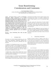
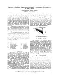
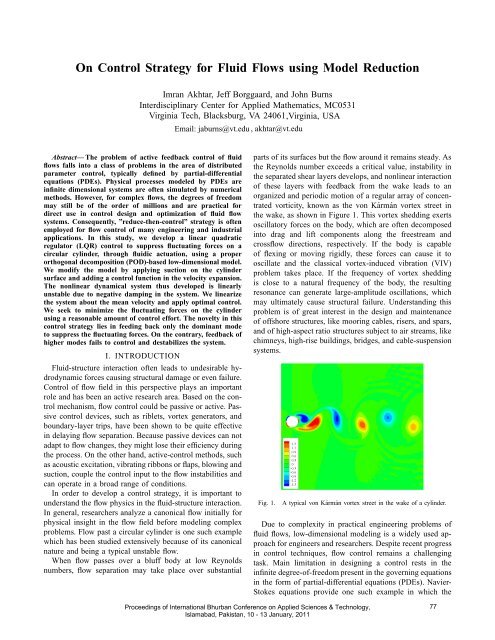
When flow passes over a bluff body at low Reynolds 

numbers, flow separation may take place over substantial 

parts of its surfaces but the flow around it remains steady. As 

the Reynolds number exceeds a critical value, instability in 

the separated shear layers develops, and nonlinear interaction 

of these layers with feedback from the wake leads to an 

organized and periodic motion of a regular array of concentrated 

vorticity, known as the von Kármán vortex street in 

the wake, as shown in Figure 1. This vortex shedding exerts 

oscillatory forces on the body, which are often decomposed 

into drag and lift components along the freestream and 

crossflow directions, respectively. If the body is capable 

of flexing or moving rigidly, these forces can cause it to 

oscillate and the classical vortex-induced vibration (VIV) 

problem takes place. If the frequency of vortex shedding 

is close to a natural frequency of the body, the resulting 

resonance can generate large-amplitude oscillations, which 

may ultimately cause structural failure. Understanding this 

problem is of great interest in the design and maintenance 

of offshore structures, like mooring cables, risers, and spars, 

and of high-aspect ratio structures subject to air streams, like 

chimneys, high-rise buildings, bridges, and cable-suspension 

systems. 

Fig. 1. 

A typical von Kármán vortex street in the wake of a cylinder. 

Due to complexity in practical engineering problems of 

fluid flows, low-dimensional modeling is a widely used approach 

for engineers and researchers. Despite recent progress 

in control techniques, flow control remains a challenging 

task. Main limitation in designing a control rests in the 

infinite degree-of-freedom present in the governing equations 

in the form of partial-differential equations (PDEs). Navier- 

Stokes equations provide one such example in which the 

Proceedings of International Bhurban Conference on Applied Sciences & Technology, 

Islamabad, Pakistan, 10 - 13 January, 2011 

77

presence of nonlinearity increases complexity of design and 

application of control. Low-dimensional modeling provides 

pratcial solutions for extremely challenging problems [1]. 

Model reduction may be viewed as representing a physical 

phenomenon by a few number of equations or physically 

reducing the infinite or large dimensions of the problem. The 

former may be termed as phenomenological modeling while 

the latter is a more direct and conventional approach to model 

reduction. 

In phenomenological modeling, a flow-related phenomenon 

is modeled by a small degrees of freedom system. 

One such example is vortex shedding in a bluff body wake. 

Several analytical approaches have been proposed to model 

vortex shedding over a circular cylinder. Bishop and Hassan 

[2] were among the earliest to suggest using a self-excited 

oscillator (Rayleigh or van der Pol oscillators) to represent 

the forces over a cylinder due to vortex shedding. Several 

other analytical models were extended to elastic and moving 

cylinders [3], [4], [5], [6], [7]. Later, such models have been 

modified for various flow parameters [8](such as Reynolds 

numbers, forcing amplitudes etc.) or change in geometric 

parameters [9]. Other examples include modeling of heartbeat, 

current in RLC circuit, etc. using self-excited oscillator 

models. 

Many low-dimensional model techniques in fluid mechanics 

are derived from the proper orthogonal decomposition 

(POD)-Galerkin projection approach [10], [11]. The POD 

provides a tool to formulate an optimal basis or minimum 

degrees of freedom (or modes) required to represent a 

dynamical system. The POD is also known as the Karhunen- 

Loeve expansion in statistics and principal component analysis 

or empirical orthogonal functions (EOF) in meteorology. 

The POD-Galerkin low-dimensional models are constructed 

in two steps: 

1) Computation of the POD basis functions from the data 

ensemble of the flow field. 

2) Galerkin projection of the Navier-Stokes equations 

onto a space spanned be a small number of POD basis 

functions. 

In the first step, the variables from the high-fidelity simulation 

(typically CFD) are transferred to a finite number 

of basis functions or modes, which are relatively small in 

number as compared to the degrees of freedom involved 

in the simulation. The second step involves a translation 

of the full-system dynamics to the implied dynamics of 

these modes. The resulting dynamical system consists of 

a set of ODEs in time in the modal amplitudes. Thus, 

low-dimensional models obtained from this procedure can 

be used to apply a control strategy. This application of 

control design at the analytical level will be beneficial for 

the design of a controller in the real-time system. Some 

other applications of low-dimensional models include shape 

optimization, aeroelastic stability analysis, and understanding 

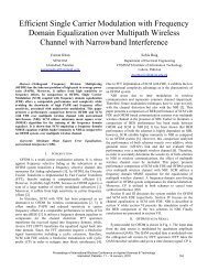
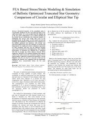
of the nonlinear dynamics of the system. A schematic of the 

hierarchy of flow models is represented in Figure 2 where 

the degrees of freedom are systematically reduced while 

preserving the physics and dominant features of the flow. 

A block diagram depicting the low-dimensional modeling proce- 

Fig. 2. 

dure. 

POD based low-dimensional models have been successfully 

implemented for various control strategies. In the current 

work, we would restrict ourselves only to the literature 

focusing on optimal control of vortex shedding past a circular 

cylinder. Graham et al. [12] developed a low-dimensional 

model for the flow past a circular cylinder at Re = 100 using 

numerical simulations and the control action was achieved 

by cylinder rotation. They introduced two approaches to 

incorporate variable input control in the low-dimensional 

model. In the first approach, known as the “control function 

method,” a suitable control function is included in the velocity 

expansion to account for the inhomogeneous boundary 

conditions on the cylinder surface. The POD modes, used in 

the modified expansion, retain the homogeneous boundary 

conditions. In the second approach, the “penalty method,” the 

velocity expansion remains the same as for the unactuated 

flow and the essential boundary condition is enforced in an 

integral “weak” fashion. 

Singh et al. [13] used these two approaches for controlling 

the cylinder wake. The models were based on POD of the 

two-dimensional incompressible, unsteady wake flow behind 

a circular cylinder at Re = 100. Linear optimal control theory 

was used to develop the feedback gains. Their simulations 

of the modes showed that, in a closed-loop system, asymptotic 

regulation of the amplitudes to the desired equilibrium 

state could be accomplished by appropriately rotating the 

cylinder. Also, they found that their linear controller was 

capable of suppressing large unsteady perturbations, despite 

the presence of nonlinearity in the flow dynamics of the two 

models. 

Bergmann et al. [14] employed optimal control approach 



78

to reduce the drag on the cylinder at Reynolds number of 

200 using cylinder rotation. They used the time angular 

velocity of the rotating cylinder as the cost function. They 

developed POD-based reduced order model and introduced 

time-dependent eddy-viscosity estimated for each POD mode 

as the solution of an auxiliary optimization problem. They 

used Lagrange multipliers to enforce constraints to solve 

optimization problem and achieved 25% of relative drag 

reduction. 

Siegel et al. [15] numerically studied the effect of feedback 

flow control on the cylinder wake at Re = 100. The controller 

applies linear proportional and differential feedback to 

the estimate of the first POD mode. Actuation is implemented 

as the displacement of the cylinder normal to the flow 

while the sensors were placed in the wake. They observed a 

reduction of 15% and 90% of drag and lift, respectively. 

Bergmann and Cordier [16] used optimal control theory 

to minimize the mean drag for a circular cylinder with 

amplitude and frequency as the control parameters using 

cylinder rotation. They employed trust-region POD approach 

in the wake which converged to the minimum predicted by 

an open-loop control approach and leads to a relative mean 

drag reduction of 30%. 

In this study, we follow an optimal control strategy to 

minimize the fluctuating forces. Most of the studies mentioned 

have used cylinder rotation as the means of actuation. 

In this study, we use suction jet as the actuator. We also 

define the objective function based on the lift coefficient. We 

develop a POD-based low-dimensional model using a control 

function approach based on suction on the cylinder surface. 

We feedback only the dominant (first) state of the system and 

compute appropriate gains. Successful application of optimal 

control on the low-dimensional model suggests that the 

fluctuating forces can be completely suppressed using suction 

actuators. The manuscript is organized as follows; Section 

II presents the numerical methodology used to simulate the 

flow past a circular cylinder. In Section III, we discuss the 

methodology to compute POD basis functions and compute 

them for the two-dimensional problem. In Section IV, we 

develop a reduced-order model for the unactuated flow field. 

Later, we discuss control function method and develop a 

reduced-order model for the actuated flow field. In Section 

V, we design an LQR control based on the linearized model 

and numerically integrate the system to show suppression of 

system response. 

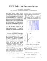
II. NUMERICAL METHODOLOGY 

where the flux is defined as 

F im = U m u i + J −1 ∂ξ m 

∂x i 

p − 1 Re Gmn ∂u i 

∂ξ n 

. (3) 

−1 ∂ξm 

∂x j 

∂ξ n 

∂x j 

Here Re = U∞D 

ν 

; J −1 = det ( ∂x i 

) 

∂ξ j 

is the inverse of the 

−1 ∂ξm 

Jacobian or the volume of the cell; U m = J 

∂x j 

u j is the 

volume flux (contravariant velocity multiplied by J −1 ) normal 

to the surface of constant ξ m ; and G mn = J 

is the “mesh skewness tensor.” 

A semi-implicit scheme is employed to advance the solution 

in time. The diagonal viscous terms are advanced 

implicitly using the second-order accurate Crank-Nicolson 

method, whereas all of the other terms are advanced using 

the second-order accurate Adams-Bashforth method. The 

Adams-Bashforth scheme was chosen because of its computational 

efficiency when coupled with the fractional step 

method. Details of the numerical algorithm, validation and 

verification can be found in Ref. [17], [9], [18]. Fluidic 

actuation (suction, blowing, or synthetic jets) on the cylinder 

surface can be used as a controlling mechanism for the flow 

field. The actuator is modeled by imposing a fixed or timevarying 

velocity normal to the cylinder surface [19]. 

The fluid force on a cylinder is the manifestation of the 

pressure and shear stresses acting on its surface. The net 

force can be decomposed into two components: lift and drag 

forces. These forces are nondimensionalized with respect to 

the dynamic pressure. The coefficients of lift and drag can 

thus be written in terms of the dimensional pressure and 

shear stresses as follows: 

C L = − 1 

ρU 2 ∞ 

C D = − 1 

ρU 2 ∞ 

∫2π 

( 

p sin θ − 1 ) 

Re ω z cosθ dθ 

0 

∫2π 

( 

p cosθ + 1 ) 

Re ω z sin θ dθ 

0 

(4a) 

(4b) 

where ω z is the spanwise vorticity component on the 

cylinder surface. 

III. POD BASIS FUNCTIONS 

A parallel CFD solver is used to simulate the flow past a 

circular cylinder [17], [18]. The governing equations are the 

Navier-Stokes equations in curvilinear coordinates (ξ m ) and 

can be written in strong conservation form as follows: 

∂(J −1 u i ) 

∂t 

∂U m 

∂ξ m 

= 0, (1) 

+ ∂F im 

∂ξ m 

= 0, (2) 

In this section, we provide the procedure for computing 

the POD basis functions for two-dimensional flow fields. The 

flow field data (u, v) is generated from an experiment or a 

numerical simulation and is assembled in a matrix W 2N×S , 

as shown in equation (5); each column represents one time 

instant or a snapshot and S is the total number of snapshots 

for N grid points in the domain. The vorticity field can also 

be used for POD, however, in the case of the velocity field, 

the singular values are a direct measure of the kinetic energy 



79

in each mode. 

⎡ 

W = 

⎢ 

⎣ 

u (1) 

1 u (2) 

1 . . . u (S) 

1 

. . . 

u (1) 

N 

u (2) 

N 

. . . u (S) 

N 

v (1) 

1 v (2) 

1 . . . v (S) 

1 

. . . 

. . . 

v (1) 

N 

v (2) 

N 

. . . v (S) 

N 

Mathematically, we compute Φ for which the following 

quantity is maximum: 

〈|u, Φ| 2〉 

⎤ 

⎥ 

⎦ 

(5) 

‖Φ‖ 2 , (6) 

where Φ are the POD basis functions and 〈.〉 denotes the 

ensemble average. Applying variational calculus, one can 

show that equation (6) is equivalent to a Fredholm integral 

eigenvalue problem represented as 

In the classical POD or direct method, originally introduced 

by Lumley [20], a two-point spatial-correlation tensor 

is formed and the eigenfunctions are the POD modes. In 

this approach, the average operator is estimated in time. On 

the other hand, if the average operator is evaluated as a 

space average over the domain of interest, the method is 

known as the method of snapshot [21]. In this approach, we 

formulate a temporal-correlation function from the snapshots 

and transform it into an eigenvalue problem. 

In this study, we compute the singular value decomposition 

(SVD) of the data ensemble W to obtain the POD modes, 

i.e. W = UΣV T , where U represents the POD basis. This 

method has a limited application, especially when the grid 

size (N) is large. [22] proposed an algorithm, inspired 

from domain decomposition ideas, for a scalable parallel 

efficient computation of the POD basis vector with low 

communication overhead. An SVD of a (spatial) subdomain 

time history is calculated locally on each processor followed 

by the exchange of a small number of dominant V p (right singular 

vector on the p th processor) with other processors. An 

iterative application of this step showed promising results for 

complex fluid flows, gravity currents, and two-dimensional 

flow past a square cylinder. Thus, 

⎡ 

U = 

⎢ 

⎣ 

φ (u) 

1,1 φ (u) 

2,1 . . . φ (u) 

S,1 

⎤ 

. . . 

φ (u) 

1,N φ(u) 2,N . . . φ(u) 

S,N 

φ (v) 

1,1 φ (v) 

2,1 . . . φ (v) 

S,1 

⎥ 

. . . ⎦ 

φ (v) 

1,N φ(v) 2,N . . . φ(v) S,N 

and Σ = diag[σ 1 σ 2 . . . σ S ] T are the singular values. 

An important characteristic of these modes is orthogonality; 

that is, Φ i .Φ j = δ ij , where δ ij is the kronecker delta. The 

optimality of the POD modes lies in capturing the greatest 

(7) 

possible fraction of the total kinetic energy for a projection 

onto the given set of modes. In equation (7), Σ contains the 

singular values of W. The corresponding singular values σ i 

are real and positive arranged in Σ in descending order. The 

σ i are related to the eigenvalues λ i obtained in the method 

of snapshots by λ i = σi 2 . They are used for ordering the 

POD basis functions for the dynamical system and represent 

energy contained in each basis function. 

Among other factors, both of the number of snapshots and 

the number of POD modes used in the simulation affect the 

accuracy of the reduced-order model. Increasing the number 

of modes increases the accuracy of the simulation, but it 

also increases the dimension of the solution space spanned 

by the modes. Similarly, increasing the number of snapshots 

increases the flow dynamics information, however, it limits 

the computational power and available computer memory. 

IV. LOW-DIMENSIONAL MODELING 

In the current study, we perform two-dimensional simulations 

of the flow past a cylinder at Re = 200 on a 192 ×256 

grid in the radial and circumferential directions, respectively, 

over the domain size of 50D. We record 40 snapshots of the 

flow field over a shedding cycle ans assemble the data in 

W matrix. We subtract the mean component and perform 

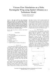
SVD of the matrix to compute the POD eigenfunctions. In 

Figure 3, we plot these eigenvalues where i th eigenvalue is 

normalized as λ i / ∑ S 

j=1 λ j. First twelve POD modes contain 

99% of the system’s energy and are sufficient for lowdimensional 

modeling for this configuration. We also plot 

the first four POD modes of the streamwise (φ u ) and normal 

(φ v ) velocity components in Figures 4 and 5, respectively. 

λ 

10 0 

10 -1 

10 -2 

10 -3 

10 -4 

10 -5 

10 -6 

10 -7 

10 -8 

Mode 

Fig. 3. Normalized eigenvalues. 

5 10 15 20 

For the flow past a circular a circular cylinder, [23] 

observed that 20 snapshots are sufficient for the construction 

of the first eight eigenfunctions. Numerical studies [24] 

suggest that the first M POD modes, where M is even, resolve 

the first M/2 temporal harmonics and require 2M number 

of snapshots for convergence. 



80

Fig. 4. 

Fig. 5. 

(a) Mode 1 (b) Mode 2 

(c) Mode 3 (d) Mode 4 

The streamwise velocity modes (φ u i , i = 1, 2, 3,4) at Re=200. 

(a) Mode 1 (b) Mode 2 

(c) Mode 3 (d) Mode 4 

The normal velocity modes (φ v i , i = 1, 2,3, 4) at Re=200. 

A. Low-dimensional Model Without Control 

In the unactuated low-dimensional model, the velocity 

field is expanded as 

u(x, t) ≈ ū(x) + 

M∑ 

q i (t)Φ i (x), (8) 

i=1 

where M is the number of POD modes used in the projection. 

We substitute equation (8) into equation (2), project this 

equation onto the Φ k , and obtain 

q˙ 

k (t) = A k + 

where 

M∑ 

B km q m (t) + 

m=1 

M∑ 

m=1 n=1 

A k = 1 Re (Φ k, ∇ 2 ū) − (Φ k ,ū.∇ū), 

M∑ 

C kmn q n (t)q m (t), (9) 

B km = −(Φ k ,ū.∇Φ m ) − (Φ k , Φ m .∇ū) + 1 Re (Φ k, ∇ 2 Φ m ), 

C kmn = −(Φ k , Φ m .∇Φ n ), 

and (a, b) = ∫ Ω 

a · b dΩ represents the inner product 

between a and b. We note that using Green’s theorem 

and the divergence-free property, the pressure term drops 

out from equation (9) for the case of p=0 on the outflow 

boundary [25]. The POD basis functions are identically 

zero on the inflow boundary because the average flow is 

subtracted from the total flow. However, in case of Neumann 

boundary conditions on outflow boundary, the contribution 

of the pressure term is not exactly zero for the cylinder 

wake. The outer domain is intentionally kept at 25D from 

the cylinder to minimize the pressure effects. Hence, the 

pressure is neglected on the outflow boundary so the pressure 

term vanishes in the reduced-order model [24]. Details of the 

projection and validation of the low-dimensional model can 

be found in [17], [18]. 

[18] developed a low-dimensional model of the pressure 

field by using the pressure-Poisson equation. Similar to the 

velocity field, the pressure field data is recorded during 

the CFD simulation. For incompressible flows, the pressure- 

Poisson equation 

∂ 2 p 

∂x 2 i 

= − ∂u i 

∂x j 

∂u j 

∂x i 

, (10) 

where i and j refer to the Cartesian components of the vector, 

is the governing equation for the pressure. The pressure field 

is then expanded as a sum of a mean component ( ¯P ) and a 

fluctuations component (p ′ ). The average pressure ¯P = 〈p〉 

is subtracted from the snapshot data and the pressure POD 

modes (Ψ i ) are computed. The pressure is then expanded in 

terms of the Ψ i (x) as follows: 

p(x, t) ≈ ¯P(x) + 

M∑ 

a m (t)Ψ m (x). (11) 

m=1 

It is important to note that, in the Galerkin expansion in 

equation (11), the temporal coefficients a i (t) are different 

from the q i (t). 

Substituting equations (8) and (11) into equation (10) and 

projecting it onto the pressure POD modes yields the lowdimensional 

model for the pressure field 

D km a k (t) = E k + 

where 

M∑ 

F km q m (t) + 

m=1 

D km = (Ψ k , ∇ 2 Ψ m ) 

M∑ 

m=1 n=1 

E k = −(Ψ k , ∇ 2 ¯P) − (Ψk , ∇ū : ∇ū) 

F km = −(Ψ k , ∇ū : ∇Φ m ) − (Ψ k , ∇Φ m : ∇ū) 

G kmn = −(Ψ k , ∇Φ m : ∇Φ n ). 

M∑ 

G kmn q n (t)q m (t), (12) 

Equations (12) constitute a set of algebraic equations 

quadratic in terms of the q i . The pressure thus obtained is 

integrated over the cylinder surface to compute the lift and 

drag forces. From equation (12), we clearly observe that 

where G is a nonlinear function of q. 



a = G(q) (13) 

81

In Figure 6, we plot the lift coefficient (C L ) and the 

first state (q 1 ) of the system. We observe that the two time 

histories have different magnitudes but approximately the 

same frequency. If we drive the response of q 1 to zero, it 

would suppress the lift force as well. Thus, we develop a 

modified low-dimensional model which includes the control 

mechanism and apply optimal control to drive the system 

response to zero. 

C L 

, q 1 

4 

2 

0 

-2 

-4 

100 110 120 130 140 

Time 

Fig. 6. Time histories of the lift coefficient (C L : solid) and first mode 

q 1 : dashed. 

B. Low-dimensional Model With Control 

In the current study, we use a pair of suction actuators on 

the cylinder surface as a control mechanism. The location and 

suction velocity of the actuators is motivated by the study 

of [17] where they used pressure POD mode distribution on 

the cylinder surface to optimally locate the actuators. The 

location is approximately ±75 ◦ from the base point of the 

cylinder. 

We use a control function approach to develop a lowdimensional 

model incorporating the control . The velocity 

field is expanded as 

u(x, t) ≈ ū(x) + 

M∑ ∑M c 

q i (t)Φ i (x) + γ i (t)Γ i (x), (14) 

i=1 

i=1 

where M c is the total number of control modes, the Γ i (x) are 

a suitable divergence-free control functions that satisfy the 

inhomogeneous boundary condition due to fluidic actuators 

(suction), and γ(t) is the variable control input. Details of 

the derivation and construction of the control mode can be 

found in Ref. [17], [26], [19]. 

We substitute equation (14) into the Navier-Stokes equations, 

project these equations onto the Φ k , and obtain 

˙q k (t) = A k + 

where 

+ 

∑M c 

m=1 

M c 

M∑ 

B km q m (t) + 

m=1 

H km ˙γ m (t) + 

M∑ 

m=1 n=1 

M∑ 

C kmn q n (t)q m (t) 

M∑ ∑M c 

J kmn q m (t)γ n (t) 

m=1 n=1 

M c M c 

∑ ∑ ∑ 

+ K km γ m (t) + L kmn γ m (t)γ n (t), (15) 

m=1 

H km = −(Φ k , Γ m ), 

m=1 n=1 

J kmn = −(Φ k , Γ n · ∇Φ m ) − (Φ k , Φ m · ∇Γ n ), 

K km = −(Φ k ,ū · ∇Γ m ) − (Φ k , Γ m · ∇ū) + 1 

Re D 

(Φ k , ∇ 2 Γ m ), 

L kmn = −(Φ k , Γ m · ∇Γ n ). 

V. APPLICATION OF LQR CONTROL 

The low-dimensional model, developed in equation (15), 

is a 12-dimensional system of nonlinear ODEs. We simplify 

the system to apply optimal control technique in an effort to 

reduce the fluctuating forces on the structure. We linearize 

the system about the mean velocity component such that 

q ∗ = 0 is the equilibrium point. According to the Hartman- 

Grobman theorem [27], (a) the fixed point, say q = q 0 , 

of the nonlinear system of the form in equation (9) is 

stable when the fixed point q ∗ = 0 of the linear system 

is asymptotically stable; and the fixed point, q = q 0 , of the 

nonlinear system of the form in equation (9) is unstable when 

the fixed point q ∗ = 0 of the linear system is unstable. In a 

topological setting, the Hartman-Grobman theorem implies 

that the trajectories in the vicinity of a hyperbolic fixed point 

q = q 0 are qualitatively similar to those in the vicinity of the 

hyperbolic fixed point q ∗ = 0 of the linearized system. In 

other words, the local nonlinear dynamics near q = q 0 is 

qualitatively similar to the linear dynamics near q ∗ = 0, and 

the qualitative change in the local nonlinear dynamics can be 

detected by examining the associated linear dynamics. Thus, 

we linearize the nonlinear system and apply optimal control 

formulation to make the system stable. 

This approach reduces the nonlinear system to a lineartime-invariant 

(LTI) system and allows us to effectively apply 

linear control theory. Thus the augmented LTI system can 

be written in the standard form of state-space equations as 

follows: [ ] [ ] [ ] [ ] 

B K q H 

= ˙q˙γ 0 T + γ 

0 γ 1 c (16) 

Here, γ c = ˙γ is a new control input to the system. We 

design an optimal controller based on the linearized system 

and make it positively damped such that the response decays 

to zero. 

A. Control Objective 

As discussed earlier, vortex shedding leads to fluctuating 

forces on the structure and may lead to VIV for elastic 



82

structures. Thus, we want to suppress vortex shedding and 

reduce the fluctuating forces acting on the structure using a 

reasonable amount of control effort. From the flow control 

point of view, the optimal control of the Navier-Stokes equations 

through boundary control is determined to minimize the 

lift forces on the cylinder. Mathematically, we seek 

min 

∫ ∞ 

0 

CL 2 (t) + Rγ2 c (t) dt 

where R represents a control cost and the dynamics are 

described by the low-dimensional model derived in equation 

(15). We now use the qualitative behavior of the reducedorder 

model to develop some simplification of this control 

problem. As shown in Figure 3, the eigenvalue spectrum 

of the unactuated POD model indicates that most of the 

energy is contained in the first two POD modes. Moreover, 

the q 1 and q 2 , corresponding to these modes, have shedding 

frequency (f s ) while the second harmonic (2f s ) of vortex 

shedding frequency appears in q 3 and q 4 . It is also interesting 

to note that for the flow past a circular cylinder, the 

dominant frequency, i.e. vortex shedding frequency, and its 

odd harmonics (3f s , 5f s ) appear in the lift coefficient while 

even harmonics (2f s , 4f s ) appear in the drag coefficient. 

From the control perspective, if we are able to control the 

states q, we can reduce the fluctuating forces, i.e. C L , on 

the cylinder. Thus, in the present setting, the optimization 

problem can be redefined as 

min 

∫ ∞ 

0 

q T (t)Qq(t) + Rγc 2 (t) dt. 

In general, we define the state weighting matrix Q M×M and 

the control effort weighting matrix R Mc×M c 

. In the current 

study, we choose M = 12, M c = 1, Q = I, and R = 10. 

We compute the appropriate gains using LQR function in 

MATLAB and observe the system response. Feeding back 

the optimal gains, all the states decay to zero. In Figure 7(a), 

we plot only the first state (q 1 ) to show its response. We also 

observe that as the states approach zero, the control input 

γ c also approaches zero as shown in Figure 7(b). However, 

this procedure requires information of all the states. From 

application point of view, we need observers to estimate 

all the states to achieve the objective, thus requiring greater 

effort and more approximation. We have also noted that states 

corresponding to higher modes have higher harmonics of 

vortex shedding which requires sensing the flow at higher 

frequency. In other words, using such an approach requires 

computation of all the states which may not be possible in 

a realistic flow field. 

B. Feeding back the Dominant State 

As discussed before, the first pair of states (q 1 and q 2 ) 

corresponds to the dominant frequency, i.e. f s , while subsequent 

pairs have harmonics of the fundamental frequency. 

The objective here is to feedback only one state and observe 

its effect on the control input and the response of the system. 

We feedback only q 1 with its gain and observe the response 

of the system with different values of R. We study three 

4 

3 

2 

1 

q 1 0 

γ c 

−1 

−2 

−3 

−4 

0 50 100 150 200 

0.6 

0.4 

0.2 

0 

−0.2 

−0.4 

−0.6 

Time 

(a) q 1 

−0.8 

0 50 100 150 200 

Fig. 7. 

Time 

(b) γ c 

Time histories of q 1 and γ c with full-state feedback. 

cases involving q 1 and with varying |Q| 

R 

as shown in Table 

I. We observe that feeding back only the dominant state (q 1 ) 

in the system can stabilize it and the response the states 

decay to zero for all the three cases as shown in Figures 

8 and 9. Based on the magnitude of |Q| 

R 

, the response is 

different for each case, however, qualitatively the behavior 

shows a similar trend. We also compute the settling time and 

maximum control input required in each case. From Figures 

TABLE I 

SYSTEM RESPONSE. 

|Q| 

Case R Gain Settling time max γ c 

A 1 0.9348 50 2.25 

B 0.1 0.3253 120 1.1 

C 0.01 0.1105 250 1.05 

8 and 9, we observe that for Case A, the settling time is 50 

time units. As we decrease the Q11 

R 

, the settling time increase 

for Cases B and C to 120 and 250, respectively. Likewise, 

in Figure 10, we observe that the gain associated with the 

first mode is high for Case A as compared to Cases B and C 

which is obvious due to increase in the control effort. Note 

that γ c → 0 in each case. Thus, given the control effort we 

can suppress the response of the system which eventually 

leads to the suppression of fluctuating forces on the cylinder. 



83

q1(t) 

3 

2 

1 

0 

−1 

−2 

−3 

0 50 100 150 200 

Time 

(a) Case A 

q2(t) 

2 

1.5 

1 

0.5 

0 

−0.5 

−1 

−1.5 

−2 

−2.5 

−3 

0 50 100 150 200 

Time 

(a) Case A 

3 

3 

2 

2 

1 

1 

q1(t) 

0 

q2(t) 

0 

−1 

−1 

−2 

−2 

−3 

0 50 100 150 200 

Time 

(b) Case B 

−3 

0 50 100 150 200 

Time 

(b) Case B 

q1(t) 

3 

2 

1 

0 

−1 

−2 

−3 

0 50 100 150 200 

Time 

(c) Case C 

Fig. 8. Time histories of q 1 with feeding back dominant state (q 1 ). 

q2(t) 

4 

3 

2 

1 

0 

−1 

−2 

−3 

0 50 100 150 200 

Time 

(c) Case C 

Fig. 9. Time histories of q 2 with feeding back dominant state (q 1 ). 

C. Feeding back the Harmonics 

In an attempt to analyze the effect of states other than 

q 1 , we feedback higher harmonics such as q 3 to the system 

along with its corresponding gain. It is important to note 

that the dominant frequency in q 3 is 2f s . Unlike q 1 , the 

system diverges as we integrate for a long time, as shown in 

Figure 11. We suggest that divergence in the system is due 

to absence of fundamental frequency in the feedback signal. 

A similar behavior is observed while feeding back higher 

harmonics. It may be related to the fact that these states are 

less dominant and does not correspond to the fundamental 

frequency of the system which appears in the lift coefficient. 

Thus, feedback of the dominant state may be sufficient to 

control the system dynamics and we may not require to 

estimate all the states in the system. 

CONCLUSIONS 

Using the snapshots of the flow field past a circular 

cylinder, we developed a low-dimensional model using POD- 

Galerkin expansion approach. Suction is used as the mechanism 

to control the flow field around a cylinder. Using the 

DNS of the controlled flow field, we developed a suitable 

control function that satisfies the inhomogeneous boundary 

condition on the cylinder surface. We substituted the modified 

velocity expansion into the Navier-Stokes equations and 

projected it onto the velocity POD modes. We linearized the 

system about the mean flow and reduced the model to an LTI 



84

γc 

1.5 

1 

0.5 

0 

−0.5 

−1 

−1.5 

−2 

−2.5 

0 50 100 150 200 

Time 

1.2 

(a) Case A 

4 

3 

2 

1 

q 1 0 

−1 

−2 

−3 

−4 

0 50 100 150 200 

1 

Time 

(a) q 1 

1 

γc 

0.8 

0.6 

0.4 

0.2 

γ c 

0.5 

0 

0 

−0.2 

−0.5 

−0.4 

−0.6 

0 50 100 150 200 

Time 

1.2 

1 

(b) Case B 

−1 

0 50 100 150 200 

Time 

(b) γ c 

Fig. 11. Time histories of q 1 and γ c with feeding back higher harmonic 

(q 3 ) only. 

0.8 

γc 

0.6 

0.4 

0.2 

0 

−0.2 

0 50 100 150 200 

Time 

(c) Case C 

Fig. 10. Time histories of γ c with feeding back dominant state (q 1 ). 

system. We applied optimal control on the LTI system with 

the objective to reduce the fluctuating forces on the cylinder. 

We studied different cases by varying Q R 

ratios and studied 

the system response. 

Note that our control is defined by feeding back the 

dominant state of the model. We observed that the dominant 

state is proportional to the lift coefficient. The latter can 

be estimated by placing sensors on the cylinder surface, 

thus with appropriate gains, the feedback control system is 

practically implementable. We showed that feedback higher 

harmonics in fact fails to stabilize the system. 

ACKNOWLEDGMENTS 

This research was supported in part by Air Force Office of 

Scientific Research grants FA9550-07-1-0273 and FA9550- 

10-1-0201 and by the Environmental Security Technology 

Certification Program (ESTCP) under a subcontract from the 

United Technologies. 

REFERENCES 

[1] K. Ito and S. Ravindran, “Reduced basis method for flow control,” 

1996, technical Report CRSC-TR96-25, Center for Research in 

Scientific Computation, North Carolina State University, Raleigh, 

NC. [Online]. Available: citeseer.ist.psu.edu/article/ito96reduced.html 

[2] R. Bishop and A. Hassan, “The lift and drag forces on a circular 

cylinder in flowing fluid,” Proceedings of the Royal Society Series A, 

vol. 277, pp. 32–50, 1963. 

[3] R. Hartlen and I. Currie, “Lift-oscillator model of vortex-induced 

vibration,” ASCE Journal of Engineering Mechanics, vol. 96, pp. 577– 

591, 1970. 

[4] W. Iwan and R. Blevins, “A model for vortex-induced oscillation of 

structures,” Journal of Applied Mechanics, vol. 41, no. 3, pp. 581–586, 

1974. 

[5] R. Landl, “A mathematical model for vortex-excited vibration of cable 

suspensions,” Journal of Sound and Vibration, vol. 42, no. 2, pp. 219– 

234, 1975. 

[6] R. Skop and O. Griffin, “On a theory for the vortex-excited oscillations 

of flexible cylindrical structures,” Journal of Sound and Vibration, 

vol. 41, no. 3, pp. 263–274, 1975. 

[7] S. Krenk and S. Nielsen, “Energy balanced double oscillator model for 

vortex-induced vibrations,” ASCE Journal of Engineering Mechanics, 

vol. 125, no. 3, pp. 263–271, 1999. 



85

[8] O. A. Marzouk, A. H. Nayfeh, I. Akhtar, and H. N. Arafat, “Modeling 

steady-state and transient forces on a cylinder,” Journal of Vibration 

and Control, vol. 13, no. 7, pp. 1065–1091, 2007. 

[9] I. Akhtar, O. A. Marzouk, and A. H. Nayfeh, “A van der Pol-Duffing 

oscillator model of hydrodynamic forces on canonical structures,” 

Journal of Computational and Nonlinear Dynamics, vol. 4, no. 4, p. 

041006, 2009. 

[10] G. Berkooz, P. Holmes, and J. L. Lumley, “The proper orthogonal 

decomposition in the analysis of turbulent flows,” Annual Review of 

Fluid Mechanics, vol. 53, pp. 321–575, 1993. 

[11] P. Holmes, J. L. Lumley, and G. Berkooz, Turbulence, Coherent 

Structures, Dynamical Systems and Symmetry. Cambridge, UK: 

Cambridge University Press, 1996. 

[12] W. R. Graham, J. Peraire, and K. Y. Tang, “Optimal control of vortex 

shedding using low-order models. Part I - Open-loop model development,” 

International Journal for Numerical Methods in Engineering, 

vol. 44, pp. 945–972, 1999. 

[13] S. N. Singh, J. H. Myatt, G. A. Addington, S. Banda, and J. K. Hall, 

“Optimal feedback control of vortex shedding using proper orthogonal 

decomposition models,” Journal of Fluids Engineering, vol. 123, pp. 

612–618, 2001. 

[14] M. Bergmann, L. Cordier, and J. P. Brancher, “Optimal rotary control 

of the cylinder wake using POD reduced-order model,” Physics of 

Fluids, vol. 17, no. 9, pp. 097 101–20, 2005. 

[15] S. Siegel, K. Cohen, and T. McLaughlin, “Numerical simulations of 

a feedback-controlled circular cylinder wake,” AIAA Journal, vol. 44, 

no. 6, pp. 1266–1276, 2006. 

[16] M. Bergmann and L. Cordier, “Optimal rotary control of the cylinder 

wake in the laminar regime by trust-region methods and POD reducedorder 

model,” Journal of Computational Physics, vol. 227, no. 16, pp. 

7813–7840, 2008. 

[17] I. Akhtar, “Parallel simulations, reduced-order modeling, and feedback 

control of vortex shedding using fluidic actuators,” Ph.D. dissertation, 

Virginia Tech, Blacksburg, VA, 2008. 

[18] I. Akhtar, A. H. Nayfeh, and C. J. Ribbens, “On the stability and 

extension of reduced-order Galerkin models in incompressible flows: 

A numerical study of vortex shedding,” Theoretical and Computational 

Fluid Dynamics, vol. 23, no. 3, pp. 213–237, 2009. 

[19] I. Akhtar and A. H. Nayfeh, “Model based control of vortex shedding 

using fluidic actuators,” Journal of Computational and Nonlinear 

Dynamics, vol. 5, no. 4, p. 041015, 2010. 

[20] H. P. Bakewell and J. L. Lumley, “Viscous sublayer and adjacent wall 

region in turbulent pipe flow,” The Physics of Fluids, vol. 10, no. 9, 

pp. 1880–1889, 1967. 

[21] L. Sirovich, “Turbulence and the dynamics of coherent structures,” 

Quarterly of Applied Mathematics, vol. 45, pp. 561–590, 1987. 

[22] C. Beattie, J. Borggaard, S. Guercin, and T. Iliescu, “A domain 

decomposition approach to POD,” in Processdings of the 45th IEEE 

Conference on Decision and Control. pp. 6750-6756, 2006. 

[23] A. E. Deane, I. G. Kevrekidis, G. E. Karniadakis, and S. A. Orsag, 

“Low-dimensional models for complex geometry flows: Application 

to grooved channels and circular cylinder,” Physics of Fluids A, vol. 3, 

no. 10, pp. 2337–2354, 1991. 

[24] B. R. Noack, P. Papas, and P. A. Monkewitz, “The need for a pressureterm 

representation in empirical Galerkin models of incompressible 

shear flows,” Journal of Fluid Mechanics, vol. 523, pp. 339–365, 2005. 

[25] X. Ma and G. Karniadakis, “A low-dimensional model for simulating 

three-dimensional cylinder flow,” Journal of Fluid Mechanics, vol. 

458, pp. 181–190, 2002. 

[26] I. Akhtar, A. H. Nayfeh, and C. J. Ribbens, “On controlling the bluff 

body wake using a reduced-order model,” in Proceedings of the 4th 

Flow Control Conference, Seattle, WA. AIAA Paper No. 2008-4189, 

2008. 

[27] V. I. Arnold, Geometric Methods in the Theory of Ordinary Differential 

Equations. New York: Springer-Verlag, 1988, ch. 3. 


Islamabad, Pakistan, 10 - 13 January, 2011 86

On Control Strategy for Fluid Flows using Model Reduction - Ibcast

Create successful ePaper yourself

Delete template?

Save as template?