
You also want an ePaper? Increase the reach of your titles
YUMPU automatically turns print PDFs into web optimized ePapers that Google loves.
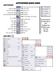
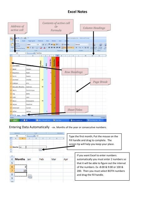
<strong>Excel</strong> Notes<br />
Address of<br />
active cell<br />
Contents of active cell<br />
Or<br />
Formula<br />
Column Headings<br />
Row Headings<br />
Page Break<br />
Sheet Titles<br />
Entering Data Automatically - ex. Months of the year or consecutive numbers.<br />
Type the first month; Put the mouse on the<br />
Fill handle and drag to complete. The<br />
screen tip will help you keep your place.<br />
If you want <strong>Excel</strong> to enter numbers<br />
automatically you must enter 2 numbers so<br />
that it will be able to figure out the interval<br />
of the numbers. Ex -8:00 & 9:00 or 100 &<br />
200. Then you must select BOTH numbers<br />
and drag the fill handle.
Insert rows or columns<br />
To insert 1 column – highlight the column to the right of where you want to insert a new column (this will insert a<br />
column before the one you highlighted); on the home tab go to Insert – Insert Sheet Columns. If you want to insert<br />
several columns – you will need to highlight an equal number of columns before you select Insert. (In other words, if you<br />
want to insert 5 new columns you will highlight the 5 columns to the right of where you want to insert your 5 columns.<br />
To insert rows you highlight 1 row to insert 1 row or 3 rows to insert 3, etc. and follow the above steps except you will<br />
select - Insert Sheet Rows<br />
Hiding Rows and Columns on large<br />
worksheets.<br />
If you have a large amount of data & are<br />
having trouble keeping your place, you can<br />
hide rows or columns to help you stay in the<br />
correct place. When you are finished, you<br />
can unhide the rows or columns.<br />
Deleting Information or cells<br />
If you want to delete information in a cell - Select the cell, then the backspace or delete button. If you want to delete a<br />
whole row or column – Select the row or column, then right click and select delete from the menu that appears.<br />
Adjusting the width or height of several rows or columns all at one time<br />
Select the rows or columns you wish to<br />
adjust, move the mouse between any of the<br />
column letters or row numbers and drag.<br />
This will adjust the width or height of all<br />
selected cells to the same width or height.
Formatting Cells<br />
To format cells – right click on a cell or a group of<br />
cells. On the number tab you will see the different<br />
options for formatting numbers. NOTE – if numbers<br />
are formatted as text you will not be able to use<br />
them in calculations.<br />
The alignment tab allows you to<br />
determine the placement of a word<br />
or number within a cell. You may<br />
change the orientation of a word by<br />
rotating the line in the orientation<br />
box on the right. The word Car Rider<br />
has been rotated 90 degrees.<br />
The other tabs can be used to change the formatting of fonts, cell borders, and fill colors.<br />
Sorting and Alphabetizing<br />
To sort your information, highlight the columns and rows that contain the information you want to sort & any rows or<br />
columns that will need to move with the sorted column or row. (If you don’t highlight data that is associated with the<br />
data you want to sort, it will not move with the sorted data). Once you have the information highlighted, go to the Data<br />
Tab and select the box above the word Sort.
A new box will open<br />
In the Sort by box, select the column you want to sort. You will probably want to leave the Sort On and Order as they<br />
are. If you want to sort by more than one level you can select Add Level and sort by an additional column. Example, if<br />
you have 3 students in your class with the same last name you will want it to sort by first name after it sorts by last<br />
name.<br />
Dragging and Dropping a group of cells<br />
If you decide to move a column or row of data – select it, point to a border of the selected cells, hold down the mouse<br />
button and drag it to where you want it. A rectangular outline shows you where the cells you are moving will be<br />
inserted. When you get them where you want them, release the mouse button. NOTE – make sure you are dragging<br />
the cells to an area where there are empty cells. If there are not empty cells available where you want to drag the cells<br />
to, insert some cells first. If you try to drop your cells on top of ones that already contain data, you will be asked if you<br />
want to replace the information in the cells.<br />
Merging Cells<br />
Select the cells you want to merge, go to the Home tab, alignment box, and select Merge & Center.<br />
Functions for adding, averaging, counting, minimum, maximum<br />
Adding a group of numbers – Select a cell that you want your sum to appear in. Click on fx at the top and a box will<br />
open. Select SUM from the list. OK.
When the function Arguments box comes up, you will type the name of the first cell and the last cell in the series of cells<br />
you want to add & you will put a colon between them. Ex. C5:C24 Then OK. This tells the program that you want to add<br />
those 2 cells and everything in between. You can also add numbers in different rows and columns as long as they<br />
remain in a rectangle or square. Ex. C5:H24 Select the first cell you want and the last cell and it will add everything in<br />
between.<br />
To Average a group of numbers you follow the above procedure but you will select AVERAGE instead of SUM.<br />
Count tells you the number of items in a row or column or row, it does not add the numbers together. Ex. (if you want to<br />
know how many grades you entered for a grading period not their total or average).<br />
Maximum will find the largest number in a group of numbers. Ex – The highest test grade.<br />
Minimum will find the smallest number in a group of numbers. Ex. – The lowest test grade.<br />
<strong>Excel</strong> will perform many other functions. If you don’t see the one you need in the list, type a question in the “Search<br />
for function” box and it will offer more options. Once you learn the functions you may type them in without using the<br />
fx button. Ex – type =SUM(C5:C24). When you hit Enter it will calculate for you.<br />
Freezing cells so that you can always see them no matter where you scroll on the worksheet<br />
If you would like for a row or column to remain visible no matter where you scroll on a worksheet (ex. – headings):<br />
select the row below the row you want to freeze, go to View, Select Freeze Panes, then choose Freeze Panes from the<br />
list. If you want to freeze a column you will select the column to the right of the one you want to freeze and follow the<br />
same procedure. If you want to unfreeze cells, go to View, Select Freeze Panes, then choose Unfreeze Panes.<br />
Printing a certain row or column on every page Ex – headings that need to appear on every page.<br />
On the Page Layout tab, in the Page Setup group, click Print Titles. In the box that appears, find the box that says “Rows<br />
to repeat at the top”, put your cursor in the empty box. Now go to your spreadsheet and click on the row you want<br />
repeated at the top of each page. When you do this you will see something appear in the “Rows to Repeat” box such as<br />
$4:$4. This means it will repeat row 4. You can do the same with columns by putting your cursor in the “Rows to Repeat<br />
at Left” box.<br />
Page Setup options such as printing gridlines, row and column headings, headers and footers<br />
You can print gridlines even if you don’t put boarders. To do so, click on the Page Layout tab, in the Page Setup group,<br />
click Print Titles. Put a check in the Gridlines box.<br />
Row and column headings (A,B, C across the top and 1,2,3 going down) can be printed by following the above directions<br />
and putting a check in the Row & Column Headings box.<br />
To add headers and footers to your spreadsheet click on the Page Layout tab, in the Page Setup group, click Print Titles.<br />
Click on the Header/Footer Tab and select Custom Header or Custom Footer, select the section of the page where you<br />
want your header or footer and type it in. Note* Headers and footers will not be visible but they will print on your<br />
spreadsheet.<br />
Making charts and graphs<br />
After entering data into a spreadsheet
Select the cells that contain the data that you want to use for the chart.<br />
On the Insert tab, in the Charts group, do one of the following: Click the chart type, and then click a chart subtype that you want<br />
to use. OR To see all available chart types, click a chart type, and then click All Chart Types to display the Insert Chart dialog<br />
box, click the arrows to scroll through all available chart types and chart subtypes, and then click the ones that you want to use.<br />
By default, the chart is placed on the worksheet as an embedded chart. If you want to place the chart in a separate chart sheet,<br />
you can change its location by doing the following: Click the embedded chart to select it. This displays the Chart Tools, adding<br />
the Design, Layout, and Format tabs.<br />
On the Design tab, in the Location group, click Move Chart.<br />
Under Choose where you want the chart to be placed, do one of the following: To display the chart in a chart sheet, click<br />
New sheet. OR To display the chart as an embedded chart in a worksheet, click Object in, and then click a worksheet in the<br />
Object in box.<br />
<strong>Excel</strong> automatically assigns a name to the chart, such as Chart1 if it is the first chart that you create on a worksheet. To change<br />
the name of the chart, do the following: Click the chart. On the Layout tab, in the Properties group, click the Chart Name text<br />
box. TIP<br />
If necessary, click the Properties icon in the Properties group to expand the group.<br />
Type a new name and press ENTER.<br />
Short cuts<br />
Ctrl + Home – takes you to the top left cell of a worksheet<br />
Ctrl + End – takes you to the bottom right cell of a worksheet<br />
Alt + Enter – takes you to the next line in the same cell