Resolution Enhancement of Color Video Sequences

Title:
Authors:
Resolution Enhancement of Color Video Sequences
Nimish R Shah and Avideh Zakhor
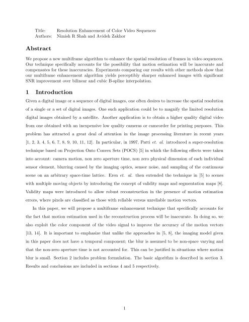
Abstract
We propose a new multiframe algorithm to enhance the spatial resolution of frames in video sequences.
Our technique specifically accounts for the possibility that motion estimation will be inaccurate and
compensates for these inaccuracies. Experiments comparing our results with other methods show that
our multiframe enhancement algorithm yields perceptibly sharper enhanced images with significant
SNR improvement over bilinear and cubic B-spline interpolation.
1 Introduction
Given a digital image or a sequence of digital images, one often desires to increase the spatial resolution
of a single or a set of digital images. One such application could be to magnify the limited resolution
digital images obtained by a satellite. Another application is to obtain a higher quality digital video
from one obtained with an inexpensive low quality cameras or camcorder for printing purposes. This
problem has attracted a great deal of attention in the image processing literature in recent years
[1, 2, 3, 4, 5, 6, 7, 8, 9, 10, 11, 12]. In particular, in 1997, Patti et. al. introduced a super-resolution
technique based on Projection Onto Convex Sets (POCS) [5] in which the following effects were taken
into account: camera motion, non zero aperture time, non zero physical dimension of each individual
sensor element, blurring caused by the imaging optics, sensor noise, and sampling of the continuous
scene on an arbitrary space-time lattice. Eren et. al. then extended the technique in [5] to scenes
with multiple moving objects by introducing the concept of validity maps and segmentation maps [8].
Validity maps were introduced to allow robust reconstruction in the presence of motion estimation
errors, where pixels are classified as those with reliable versus unreliable motion vectors.
In this paper, we will propose a multiframe enhancement technique that specifically accounts for
the fact that motion estimation used in the reconstruction process will be inaccurate. In doing so, we
also exploit the color component of the video signal to improve the accuracy of the motion vectors
[13, 14]. It is important to emphasize that unlike the approaches in [5, 8], the imaging model given
in this paper does not have a temporal component; the blur is assumed to be non-space varying and
that the non-zero aperture time is not accounted for. This can be justified in situations where motion
blur is small. Section 2 includes problem formulation. The basic algorithm is described in section 3.
Results and conclusions are included in sections 4 and 5 respectively.
1

2 Problem Statement
Let f(x,y,t) denote a time-varying continuous-space, continuous-time scene projected onto a twodimensional
image plane. Assume that the region of interest of f(x,y,t) is 0 ≤ x ≤ N 2 ∆,0 ≤ y ≤ N 1 ∆.
Then we can let l (k)
i,j for 0 ≤ k ≤ K − 1,0 ≤ i ≤ N 1 − 1,0 ≤ j ≤ N 2 − 1 denote the (N 1 × N 2 )-pixel,
discrete-space, discrete-time frames in the corresponding digital video sequence of length K. l (k)
i,j
denotes the pixel element at the i th row and j th column of the k th frame. The relationship between
f(x,y,t) and l (k)
i,j
is given by
l (k)
i,j = ∫ (k+1)T
kT
∫ (i+1)∆ ∫ (j+1)∆
i∆
j∆
f(x,y,t) dx dy dt, i = 0,... ,N 1 − 1, j = 0,... ,N 2 − 1, (1)
where T is the exposure time for obtaining each digital frame. The problem we solve is to use M con-
M−1
(k−
secutive original (N 1 ×N 2 ) pixel video frames {l 2 ) ,... ,l (k) M−1
(k+
,...,l 2 ) } to obtain the sequence
of (N 1 × N 2 )-pixel frames {l (k) } to obtain a (qN 1 × qN 2 )-pixel frames h (k) . Without loss of generality,
we will present our methods with a value of M = 5.
3 Enhancement Algorithm
The overall system diagram for the proposed multiframe enhancement algorithm is shown in Figure 1.
The first block in the diagram, labeled “Motion Estimation”, takes the set of low resolution intensity
frames as input, with the central frame (Frame #k) as the reference frame, and outputs a set of
motion estimates for each frame relative to the reference frame. The next block in the diagram, labeled
“Iterative Algorithm”, takes the low resolution intensity frames along with the motion estimates as
input to form an initial estimate of the high resolution frame. Then, it takes this initial estimate, along
with the low resolution intensity frames and motion estimates, and applies an iterative algorithm to
converge upon the final enhanced high resolution frame estimate. This section describes each of these
procedures in more detail.
3.1 Modified Block Matching Algorithm(MBMA)
Our approach is to match each low resolution frame l (i) ,i ∈ {k − 2,k − 1,k + 1,k + 2} relative to the
reference frame l (k) using the traditional block matching algorithm. There are two novelties to our
motion estimation technique. First, we find a set of candidate motion estimates instead of a single
motion vector for each pixel of the match frame relative to the reference frame. Second, we use both
the luminance and chrominance values to compute the dense field of subpixel accuracy motion vectors.
2

3.1.1 Candidate Set of Motion Vectors
Our motion estimation algorithm is based on the fact that the true motion vector may have a higher
MSE than other false motion estimates. We have empirically found that the true motion estimate
usually has an MSE close to the “best” or lowest value. Hence, instead of simply accepting the possibly
false minimum MSE motion vector as our estimate, we save several candidate motion estimates for each
pixel along with the corresponding MSE’s. These candidates consist of the estimate with smallest MSE
along with all the estimates which have an error less than a small multiple τ of the minimum MSE.
Using this procedure, for each pixel in the match frame we get a small set of possible motion vectors,
ranked by the corresponding MSE, relative to the reference frame. We refer to these set of motion
vectors as { ˆm i→k } k+2
i=k−2 .
There are two motivations behind using a candidate set of motion vectors rather than a single
motion vector per pixel. First, as we will see later, one motion vector per pixel results in too many
“holes” in the initial high resolution estimate, which in turn causes problems during the iterations
of our reconstruction algorithm. Second, the imperfections in traditional BMA sometimes result in
inaccuracies when choosing one motion vector per pixel. An example of the lowest MSE leading to
an incorrect motion estimate is shown in Figure 2. Here we have an original high resolution image
consisting of an object with a diagonal edge. We also show the resulting low resolution images after
applying a 2 ×2 uniform blurring function to shifted versions of the high resolution image. We observe
that the low resolution images l 2 ,l 3 and l 4 are identical despite the fact they correspond to different
shifts relative to the single high resolution image.
3.1.2 Chrominance Components to Increase Accuracy
Another difference between our motion estimation and traditional techniques is our use of color [13, 14].
The standard BMA is usually used only on the intensity or luminance component of the video signal.
However, since we wish to obtain a high degree of accuracy in our motion estimates and because we
will apply our method to color video sequences, our modified block matching algorithm uses the color
components of the video signal to aid in motion estimation. In particular, we use luma and chroma
components to arrive at one motion vector for all components based on a technique described at [14].
Harasaki and Zakhor [14] have shown that motion estimation using color components can significantly
reduce motion estimation errors. Our experiments on sequences with known motion showed a 20%
improvement in the number of correct motion estimates when using color components in the motion
estimation as compared with luminance only motion estimation. This process adds some computational
complexity to the algorithm but this cost is justified by the increased accuracy achieved.
3

3.2 Iterative Enhancement
After performing motion estimation to find the correspondences between the set of low resolution
frames, we combine the available information to generate an initial high resolution frame estimate and
then iteratively refine this estimate.
3.2.1 Initial High Resolution Estimate
For the initial high resolution frame estimate, we combine the low resolution frames using the motion
estimates { ˆm i→k } k+2
i=k−2
from section 3.1.1. The combination method maps all the intensity values from
the set of low resolution frames onto a high resolution frame grid using the sets of subpixel accuracy
candidate motion vectors. So, the pixels of the reference low resolution frame occupy a regularly spaced
subset of the high resolution grid. For the remaining low resolution frames, we have subpixel accuracy
motion estimates which enable us to map their pixels to the finer high resolution grid. Since, we
have several frames and multiple motion vectors per pixel, this mapping process will yield some high
resolution pixels with multiple conflicting intensity values landing on them. Since the high resolution
grid is finer than the low resolution grid, it is also possible that some high resolution grid points will
have no low resolution intensity values placed on them. These points are referred to as holes. The
possible situations that can arise are depicted pictorially in Figure 3.
In the case of multiple low resolution intensities vying for a single high resolution pixel location,
we choose the intensity and corresponding motion vector of the low resolution pixel which had the
lowest MSE during the MBMA algorithm. In the case of holes, although no low resolution intensity
points map to the holes, it is still desirable to have a good initial estimate for these pixels before we
start the iterative enhancement. For this reason, we apply an interpolation technique such as nearest
neighbor to estimate the holes based on surrounding filled grid points. The estimates in the initial
high resolution frame will be modified by the iterative algorithm, so high accuracy at this stage is not
required.
3.2.2 Iterative Algorithm
Our iterative stage is based on the Landweber algorithm. For ease of summarizing the general scheme,
we consider the case of estimating a high resolution frame from only two low resolution frames; the
case with a larger set of low resolution frames is a straightforward extension. Initially, we desire a good
estimate of the original high resolution frame h from the corresponding set of low resolution frames
l (1) and l (2) , which are available to us. At step n − 1 of the iteration, we have a high resolution frame
estimate ĥn−1. For step n of the iteration, we desire the estimate ĥn to be a better estimate than
ĥ n−1 of the original high resolution frame h which is, of course, unknown. The original low resolution
4

frames, however, are known and can be used to yield information about h. The approach we take is to
use the motion estimate information to simulate the imaging of low resolution frames ˆl (1) and ˆl (2) from
ĥ n−1 . We then compare and determine the error between the simulated low resolution frames ˆl (1) ,
and the original low resolution frames l (1) ,l (2) . We use this computed error in the iteration step to
modify ĥn−1, yielding a better estimate ĥn. Successive iterations allow us to converge on a final high
resolution estimate for the original high resolution frame h. The precise algorithm for this iterative
technique is given below.
Algorithm (Iterative Enhancement): Determine a high resolution frame estimate for frame h (k) .
1. Using the method outlined in Section 3.2.1, determine an initial high resolution frame estimate
ĥ (k)
0 and a consistent set of motion vectors {m i→k } k+2
i=k−2
from the set of low resolution frames
{l (i) } k+2
i=k−2 and the initial motion estimates { ˆm i→k} k+2
i=k−2 .
2. Set the iteration step counter to s = 0, so that ĥ(k) s
in Step 1.
ˆl
(2)
is equal to the initial frame estimate determined
3. Using the high resolution frame estimate ĥ(k) s , apply the imaging process to it using the motion
estimates {m i→k } k+2
(i)
i=k−2
to obtain a sequence of simulated low resolution frames {ˆl s } k+2
i=k−2 .
4. Compare the simulated and original low resolution frames, {ˆl s (i) } k+2
i=k−2
and {l(i) s } k+2
i=k−2 , respectively,
to determine the errors in the pixels of the high resolution frame estimate ĥ(k)
5. Use the errors determined in Step 4 and the motion vectors {m i→k } k+2
i=k−2
to adjust the high
resolution estimate ĥ(k) s using Landweber’s iterative algorithm to yield a new high resolution
frame estimate ĥ(k) s+1 .
6. Increment the iteration step: s ← s + 1.
7. Repeat Steps 3 to 6 until either the error calculated in Step 4 is less than some desired value or
until a desired number of iterations have been performed.
4 Results
s .
We shall now examine some experimental results using the methods described above for Foreman and
Mobile Calendar sequences. For both sequences, we chose τ = 10% for all frames, M = 5, and used
a 2 × 2 uniform support blurring function to obtain a sequence of low resolution frarmes. The first
test video sequence, entitled Foreman, consists of a camera panning through a scene of man’s upper
body in the foreground with a building in the background. The original high resolution frames each
consist of one 176 × 144 pixel luminance component and two 88 × 72 pixel chrominance components.
Frame #0, Frame #10, Frame #15 and Frame #25 of the low resolution sequence are shown in
5

Figure 4. We applied our multiframe algorithm to the first 25 frames of the low resolution Foreman
sequence. For comparison, we also applied the single frame techniques of bilinear interpolation and
cubic B-spline interpolation, as well as a multiframe method using traditional BMA for the motion
estimation. Figure 5 shows the original high resolution Frame #0 as well as the high resolution estimate
for Frame #0 obtained by using the different methods. We notice that the single frame techniques look
more blurred than the multiframe result. In particular, the multiframe estimate contains much sharper
edges than either of the other two approaches. Note that Frame #0 was estimated from frames -2, -1,
+1, and +2 and that frame #0 was not the first frame of the video sequence under consideration.
To perform a more quantitative comparison, we computed the signal-to-noise ratio(SNR) for the
various methods, including a multiframe approach using simple BMA instead of the novel approach
proposed in this paper. The results are shown in Figure 6 and Table 5. We observe that our proposed
multiframe method performs better than bilinear interpolation by an average of 3.5dB, better
than cubic B-spline interpolation by an average of 2.5dB and better than a multiframe method using
traditional BMA by an average of almost 2.0dB.
The multiframe algorithm performs significantly better than the single frame methods for all the
frames in the sequence, with greater performance differential for some parts of the sequence than others.
Figure 6 reveals that for the first 10 frames the multiframe method is at least 3.0dB better than cubic
B-spline interpolation and at least 4.0dB better than bilinear interpolation. In some regions, however,
such as in the vicinity of Frame #10, the improvement is not as dramatic, yielding only 1.0dB of
improvement. Direct observation of the video sequence reveals that the video frames corresponding to
the areas of less significant improvement contain very little motion between frames.
The second video sequence, entitled Mobile Calendar, consists of nontrivial motions among several
objects possessing fine detail and significant color components. In the sequence, a wall calendar moves
with 3-D translational motion(i.e., translational motion in the image plane as well as a component
perpendicular to the camera), a toy train moves with roughly translational motion and the train
6

pushes a ball which undergoes rotational motion. The original high resolution frames each consist of
one 400 × 320 pixel luminance component and two 200 × 160 pixel chrominance components. Four
low resolution frames are shown in Figure 7. We followed the same procedure as with the Foreman
sequence to generate a sequence of high resolution estimates. The results for Frame #0 are shown in
Figure 8. Once again, note that frame #0 was estimated from frames -2, -1, +1, and +2 and that frame
#0 was not the first frame of the video sequence under consideration. We observe that the multiframe
method is capable of reproducing an estimate that is comparable to the original high resolution frame.
The details in the multiframe estimate are much sharper than those in either single frame interpolation
method. The quantitative results support the perceived improvement in quality. Table 5 shows the
average SNR for the various methods over the entire sequence. The multiframe approach performs
about 1.1dB better than bilinear interpolation, about 1.6dB better than cubic B-spline interpolation
and about 0.86dB better than multiframe using traditional BMA. Figure 9 shows the SNR plot. We
observe that the proposed method outperforms the others throughout the sequence.
5 Conclusions
We have proposed an approach for enhancing the spatial resolution of a color video sequence by using
multiple frames to obtain each enhanced resolution frame. The results presented in Section 4 indicate
that this multiframe approach significantly outperforms standard single frame approaches in both SNR
and perceived visual quality. This is in spite of the fact that there is no explicit model taken into account
for the motion blur [5]. It is important to emphasize that the desired expansion factor determines the
accuracy with which the motion vectors need to be determined. For example, a 3X magnification factor
would have required motion vector estimation with resolution of 1/3 pixels. Convergence properties of
the algorithm are demonstrated in [15].
References
[1] S. P. Kim and W. Y. Su, “Recursive high resolution reconstruction of blurred multiframe images,”
7