Scaling statistical analysis of magnetic and gravity data

Scaling statistical analysis of magnetic and gravity data
Stefan Maus, Dept. of Earth SC., University of Leeds.
Summary
Statistical analysis is a powerful tool for the interpretation
of potential field data. Recent findings on scaling
properties of the density and susceptibility distribution
in the Earth’s crust have had a strong impact on statistical
methods. I introduce the concept of scaling features of
potential fields and show how scaling models can be used
in the processing and interpretation of magnetic and gravity
data for geological mapping and to determine depth.
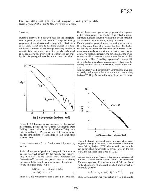
Figure 1: (a) Log-log power spectrum of the vertical
susceptibility profile of the German Continental Deep
Drilling Project pilot borehole. Blackman-Tukey estimate,
smoothed by a Parzen window of 400-m maximum
lag. The straight line (b) has a slope of -0.4 (after Maus
& Dimri, 1995).
Power spectrum of the field caused by scaling
sources
Statistical analysis of gravity and magnetic data requires
realistic statistical models for the density and susceptibility
distribution in the Earth’s crust. Pilkington and
showed that power spectra of density
and susceptibility logs decay approximately linearly when
plotted in log-log scale (Fig. 1)
PF 2.7
Hence, these power spectra are proportional to a power
of the wavenumber. The constant is called a scaling
exponent. Random functions with such a power spectrum
are referred to as self-similar, scaling or fractal.
From a practical point of view, the scaling exponent reflects
the ruggedness of a random function. The higher
the scaling exponent the smoother the function. White
noise corresponds to a scaling exponent of zero. When
comparing scaling exponents, the dimension of the crosssection
on which measurements were made has to be taken
into account. The 1D scaling exponent of a susceptibility
profile, for example, is approximately 1 less than the
scaling exponent of a 2D susceptibility survey of the same
area 3 .
Scaling density and susceptibility distributions give rise
to gravity and magnetic fields which in turn have scaling
(Fig. 2). As in the case of the source distri-
Figure 2: Radially averaged power spectrum of an aeromagnetic
survey in the area of the German Continental
Deep Drilling Project (KTB) after reduction to the pole
and continuation downwards to ground level in log-log
scale. The solid line has a slope of -1.95.
butions, there is a difference in the scaling exponents of
1D and 2D cross-sections of the field 3 . The theoretical
2D power spectrum of the potential field in a horizontal
observation plane caused by a half-space of scaling
sources is given by
(1)
where k is the wavenumber and and are constants. where is a constant (for fixed values of is related to
1419

Figure 3: Radially averaged log power spectrum of the
KTB aeromagnetic survey. The solid line indicates the
model power spectrum for 19.23, = and
= 2.07 (after Maus & Dimri, 1995).
the intensity of density or susceptibility variations,
reflects the anisotropy of the magnetic field (for the gravity
field is the scaling exponent of the field
and is the distance between the observation plane and
the top of the model half-space. Fig. 3 shows the fit of
the model power spectrum defined by eq. (2) to the power
spectrum of a real aeromagnetic data set. In this case the
radially averaged power spectrum was used. However,
radial averaging leads to a loss of information and future
methods are likely to use the original 2D power spectrum,
instead.
Applications
The model power spectrum defined by eq. (2) is governed
by three parameters, and which can be derived by
statistical analysis of a survey and can subsequently be
displayed as maps. All three parameters describe different
aspects of the gravity or magnetic field.
The depth to the top of the sources is particularly interesting
in the study of sedimentary basins, where it may
reflect the depth to the crystalline basement or the depth
to certain intra-basin geological structures.
The Intensity quantifies the amplitude of susceptibility
and density variations while taking into account the distance
of the sources from the observation plane. Hence,
the parameter can be high even for a weak field anomaly,
if the depth to the source anomaly is high at the same
Scaling statistical analysis
1420
Figure 4: A window is moved over the survey area. For
every position of the window an inversion is carried out
using the data within the window. Here, the resulting
depths to source are displayed as a profile.
time. A further attractive feature of the parameter is
that it can be derived from magnetic data without a reduction
to the pole.
The third parameter, the scaling exponent reflects statistical
properties of the source distributions. As discussed
below, it may be useful in separating different
types of geology, such as volcanic from metamorphic, or
Recent from Precambrian.
The optimum values for these parameters are obtained
by inversion. An appropriately sized ‘window is moved
over the data set (Fig. 4), and an inversion of the data
within the window is carried out to derive the best values
for and at every position of the window. The
values for subsequent inversions (= window positions) can
then be plotted as profiles (Fig. 4 & 5), or as maps of
the particular parameter. However, due to a trade-off
between the scaling exponent and the depth to source
only one of these two parameters can be resolved at a
time.
To obtain the depth to source, a constant scaling exponent
has shown to be a reasonable assumption in areas
without major changes in the geology of the basement.
Pilkington and Todoeschuck 7 used a value of = 3, while
7 = 2 was used in another case study 8 (Fig. 4 & 5). Using
a lower scaling exponent leads to greater depth estimates
and vice-versa. Thus, the method can be calibrated by
choosing the scaling exponent in such a way that the inversion
yields the correct depth to source for a window
with known basement depth.
If, on the other hand, the area has outcropping sources

Figure 5: The magnetic profiles used for the inversion are
plotted together in the top graph. The statistical method
quantifies the ruggedness of these profiles in terms of the
scaling exponent and the depth to source, whereas the
amplitude of the field is reflected in the source intensity.
For this particular study the scaling exponent was kept
constant at = 2.
Scaling statistical analysis
then the depth to the top of the sources is known to be
the survey terrain clearance. In this case one can derive
maps of the Intensity and the scaling exponent Fig. 6
shows a profile of the scaling exponent over an area with
outcropping magnetic rocks. It correlates well with the
surface geology. The variations of the scaling exponent
are thought to indicate differences in the distribution of
magnetic minerals within the geological units”.
Conclusions and outlook
Scaling source models have lead to a new understanding of
the power spectrum of gravity and magnetic data. They
have made it possible to map the topography of a crystalline
basement covered by nonmagnetic sediments with
increased precision’. As a by-product, a map of the intensity
of magnetization of the basement can be obtained.
For areas with outcropping sources, maps of the intensity
and the scaling exponent of the source variations can
be derived. Although this has so far only been tried for
magnetic data 5 , it may in fact be an attractive way of
displaying gravity data.
Many of the theoretical questions regarding scaling features
of potential fields are now quite well understood.
Hence, the next step should be to develop efficient algorithms
for high resolution mapping of the scaling parame-
1421
Figure 6: A SW-NE profile of the scaling exponent in
the area of the German Continental Deep Drilling Project
(KTB) with a cartoon of the geological section. The Franconian
line, a major vertical fault, is indicated by FL (after
Maus & Dimri, 1995).
ters and Existing methods of spectral analysis can
be improved by using an anisotropic 2D spectral model,
instead of the radially averaged power spectrum. Furthermore,
the loss of information during gridding can be
avoided by estimating power spectra directly from the
original point-located data.
References
[l]Pilkington, M., and J. P. Todoeschuck, Stochastic inversion
for scaling geology, Geophys. J. Int., 102, 205-217,1990.
[2] Pilkington, M. and J. P. Todoeschuck, Fractal magnetization
of continental crust, Geophys. Res. Lett., 20, 627,630,
1993.
[3] Maus, S., and V. P. Dimri, Scaling properties of potential
fields due to scaling sources, Geophys. Res. Lett., 21,891.894,
1994.
[4] Gregotski, M. E., 0. G. Jensen, and J. Arkani-Hamed, Fractal
stochastic modeling of aeromagnetic data, Geophysics, 56,
1706-1715,1991.
[5] Maus, S. and V. P. Dimri, Potential field power spectrum inversion
for scaling geology, J. Geophys. Res., 100, B7, 12605-
12616,1995.
[6] Maus, S. and V.P. Dimri, Depth estimation from the scaling
power spectrum of potential fields? Geophys. J. Int. 124,113.
120 (1996).
[7] Pilkington, M., M. E. Gregotski, and J. P. Todoeschuck,
Using fractal crustal magnetization models in magnetic interpretation,
Geophys. Prospect., 42, 677.692,1994.
[8] Maus, S., K.P. Sengpiel, and E.W.A. Tordiffe, Variogram
analysis of magnetic data to identify paleochannels of the
Omaruru River in Namibia, to be presented at the SEG annual
meeting in Denver, 1996.