PhD and MPhil Thesis Classes - Antares

Alma Mater Studiorum - Università di Bologna
Facoltà di Scienze Matematiche Fisiche e Naturali
Dottorato di Ricerca in Fisica
XXII ciclo
Study of diffuse flux of high energy
neutrinos through showers with the
ANTARES neutrino telescope
Author: Giada Carminati
Ph.D. Coordinator:
Prof. Fabio Ortolani
Promoter:
Prof. Maurizio Spurio
Bologna - May 4 th 2010

A mia zia Lia
E quindi uscimmo a riveder le stelle.
Dante Alighieri (Inferno - Canto XXXIV)

Contents
Introduction 5
1 High Energy Astronomy 9
1.1 Composition and Energy Spectrum of Cosmic Rays . . . . . . . . . . . . . . 10
1.1.1 The GZK Cutoff . . . . . . . . . . . . . . . . . . . . . . . . . . . . . 12
1.2 Production of Gamma-Rays and Neutrinos . . . . . . . . . . . . . . . . . . 13
1.3 Origin of the Bulk of Cosmic Rays . . . . . . . . . . . . . . . . . . . . . . . 15
1.3.1 Shock Acceleration and Supernova Explosion . . . . . . . . . . . . . 16
1.3.2 Candidate Galactic Neutrino Sources . . . . . . . . . . . . . . . . . . 17
1.4 Origin of Ultra High Energy Cosmic Rays . . . . . . . . . . . . . . . . . . . 18
1.4.1 Acceleration Scenarios and Source Candidates . . . . . . . . . . . . . 18
1.4.2 Decay Scenario . . . . . . . . . . . . . . . . . . . . . . . . . . . . . . 20
1.4.3 Cosmogenic Neutrinos . . . . . . . . . . . . . . . . . . . . . . . . . . 22
2 The ANTARES neutrino telescope 23
2.1 Cherenkov Radiation . . . . . . . . . . . . . . . . . . . . . . . . . . . . . . . 24
2.2 Detector Layout . . . . . . . . . . . . . . . . . . . . . . . . . . . . . . . . . 25
2.3 Detector Status . . . . . . . . . . . . . . . . . . . . . . . . . . . . . . . . . . 29
2.4 Detector Acquisition . . . . . . . . . . . . . . . . . . . . . . . . . . . . . . . 30
2.4.1 Signal Digitization . . . . . . . . . . . . . . . . . . . . . . . . . . . . 30
2.4.2 Data Transmission . . . . . . . . . . . . . . . . . . . . . . . . . . . . 31
2.4.3 Data filtering and storage . . . . . . . . . . . . . . . . . . . . . . . . 32
2.5 Detector Calibration . . . . . . . . . . . . . . . . . . . . . . . . . . . . . . . 32
2.5.1 Time Calibration . . . . . . . . . . . . . . . . . . . . . . . . . . . . . 32
2.5.2 Charge Calibration . . . . . . . . . . . . . . . . . . . . . . . . . . . . 33
2.5.3 Position Calibration . . . . . . . . . . . . . . . . . . . . . . . . . . . 34
2.6 Optical Background . . . . . . . . . . . . . . . . . . . . . . . . . . . . . . . 36

2 CONTENTS
3 Parameterization of Atmospheric Muons 39
3.1 Cosmic Ray Interaction with the Earth’s Atmosphere . . . . . . . . . . . . 39
3.2 Primary Cosmic Ray Models . . . . . . . . . . . . . . . . . . . . . . . . . . 42
3.3 Parametric Formulae of Underwater Muons . . . . . . . . . . . . . . . . . . 45
3.3.1 Muon Energy Loss in Water . . . . . . . . . . . . . . . . . . . . . . . 46
3.3.2 Flux of Muon Bundles . . . . . . . . . . . . . . . . . . . . . . . . . . 47
3.3.3 Energy Spectrum . . . . . . . . . . . . . . . . . . . . . . . . . . . . . 47
3.3.4 Lateral Spread . . . . . . . . . . . . . . . . . . . . . . . . . . . . . . 49
3.3.5 Multiplicity . . . . . . . . . . . . . . . . . . . . . . . . . . . . . . . . 50
3.4 Comparison of Parametric Formulae with Experimental Data . . . . . . . . 50
4 The Simulation of Underwater Atmospheric Muons: MUPAGE 53
4.1 Program Structure . . . . . . . . . . . . . . . . . . . . . . . . . . . . . . . . 53
4.2 Generation of Muon Bundles on the Can Surface . . . . . . . . . . . . . . . 56
4.2.1 Sampling of the Bundle Direction and of the Impact Point . . . . . . 56
4.2.2 Hit-or-Miss Method to Sample the Impact Point . . . . . . . . . . . 58
4.3 Single Muons . . . . . . . . . . . . . . . . . . . . . . . . . . . . . . . . . . . 59
4.4 Multiple Muons . . . . . . . . . . . . . . . . . . . . . . . . . . . . . . . . . . 60
4.4.1 Radial Distance of Muons with Respect to the Bundle Axis . . . . . 60
4.4.2 Coordinates of the Multiple Muons on the Can Surface . . . . . . . 60
4.4.3 Arrival Time of the Muons in the Bundle . . . . . . . . . . . . . . . 62
4.4.4 Muon Energy for Multimuon Events . . . . . . . . . . . . . . . . . . 63
4.5 Livetime of the Simulation . . . . . . . . . . . . . . . . . . . . . . . . . . . . 63
4.6 Comparison of Angular Distributions with ANTARES data . . . . . . . . . 64
5 Ultra High Energy Neutrinos 67
5.1 Atmospheric Neutrinos . . . . . . . . . . . . . . . . . . . . . . . . . . . . . . 68
5.2 Diffuse Neutrino Flux . . . . . . . . . . . . . . . . . . . . . . . . . . . . . . 69
5.3 Neutrino Oscillation Effects on the Diffuse Neutrino Flux . . . . . . . . . . 70
5.4 Neutrino Interactions . . . . . . . . . . . . . . . . . . . . . . . . . . . . . . . 72
5.5 Earth’s Opacity to Neutrinos . . . . . . . . . . . . . . . . . . . . . . . . . . 74
6 Diffuse Neutrino Flux Analysis 77
6.1 Monte Carlo Samples . . . . . . . . . . . . . . . . . . . . . . . . . . . . . . . 77
6.1.1 Atmospheric Muons . . . . . . . . . . . . . . . . . . . . . . . . . . . 78
6.1.2 Atmospheric CC Muon Neutrinos . . . . . . . . . . . . . . . . . . . . 78

CONTENTS 3
6.1.3 CC Electron Neutrinos . . . . . . . . . . . . . . . . . . . . . . . . . . 80
6.1.4 NC Neutrinos . . . . . . . . . . . . . . . . . . . . . . . . . . . . . . . 83
6.2 Rejection of the Background Signal . . . . . . . . . . . . . . . . . . . . . . . 83
6.2.1 Number of lines . . . . . . . . . . . . . . . . . . . . . . . . . . . . . . 84
6.2.2 Fit Quality Parameters . . . . . . . . . . . . . . . . . . . . . . . . . 84
6.2.3 Amplitude . . . . . . . . . . . . . . . . . . . . . . . . . . . . . . . . . 85
6.2.4 Summary of the Selection Criteria . . . . . . . . . . . . . . . . . . . 87
6.3 Comparison between Monte Carlo Atmospheric Muons and Data . . . . . . 88
6.4 Efficiencies and Purities of the Selection Criteria . . . . . . . . . . . . . . . 89
7 Sensitivity to the Diffuse Neutrino Flux through Showers 91
7.1 Diffuse Neutrino Flux Sensitivity . . . . . . . . . . . . . . . . . . . . . . . . 91
7.2 The Real Detector . . . . . . . . . . . . . . . . . . . . . . . . . . . . . . . . 93
7.3 Monte Carlo Samples for Different ANTARES Setups . . . . . . . . . . . . 94
7.3.1 9Line Configuration . . . . . . . . . . . . . . . . . . . . . . . . . . . 94
7.3.2 10Line Configuration . . . . . . . . . . . . . . . . . . . . . . . . . . . 95
7.4 Diffuse Neutrino Flux Analysis for Different Setups . . . . . . . . . . . . . . 95
7.5 Conclusion and Outlook . . . . . . . . . . . . . . . . . . . . . . . . . . . . . 98
A ANTARES Analysis Chain 101
A.1 Monte Carlo Event Generators . . . . . . . . . . . . . . . . . . . . . . . . . 101
A.1.1 MUPAGE . . . . . . . . . . . . . . . . . . . . . . . . . . . . . . . . . 101
A.1.2 Genhen . . . . . . . . . . . . . . . . . . . . . . . . . . . . . . . . . . 102
A.2 Cherenkov Light Production and Detector Simulation . . . . . . . . . . . . 103
A.2.1 KM3 . . . . . . . . . . . . . . . . . . . . . . . . . . . . . . . . . . . . 103
A.2.2 Geasim . . . . . . . . . . . . . . . . . . . . . . . . . . . . . . . . . . 103
A.3 Trigger Selection . . . . . . . . . . . . . . . . . . . . . . . . . . . . . . . . . 104
A.4 Reconstruction Algorithm . . . . . . . . . . . . . . . . . . . . . . . . . . . . 105
A.4.1 Fitting Procedure . . . . . . . . . . . . . . . . . . . . . . . . . . . . 106
A.4.1.1 Particle Track . . . . . . . . . . . . . . . . . . . . . . . . . 106
A.4.1.2 Bright Point . . . . . . . . . . . . . . . . . . . . . . . . . . 107
A.4.1.3 Fit Function . . . . . . . . . . . . . . . . . . . . . . . . . . 108
A.4.1.4 Minimization Procedure . . . . . . . . . . . . . . . . . . . . 109
A.4.2 Event Display . . . . . . . . . . . . . . . . . . . . . . . . . . . . . . . 109
References 113

4 CONTENTS
Summary 119

Introduction
Astronomy, with several thousand years of history, is one of the oldest of the natural
sciences. Most of our knowledge of the Universe comes from the observations of the photons
through the entire electromagnetic spectrum. However, the ultra high energy domain
remains largely unexplored by conventional astronomical methods, because gamma-ray
astronomy observations are limited by the high energy photon interactions with the 2.7 K
cosmic microwave background radiation. As a result, the Universe is opaque to gammarays
from extragalactic sources; photons with energy higher than 10 6 GeV cannot even
survive the journey from the Galactic Center to the Earth.
On the contrary, the observation of high energy neutrinos may help to explain the
dynamics of the most energetic phenomena that occur in the Universe. Due to their nature
(weakly interacting and neutral charge), neutrinos can escape from hot dense sources
without being absorbed during their propagation to the Earth or deflected by extragalactic,
galactic and geo-magnetic fields. Therefore, neutrinos act as cosmic messengers which point
straight back to their source and may identify extragalactic and galactic sources of cosmic
rays. However, due to their small interaction cross sections, a large target mass is essential
to detect them. For this reason cosmic neutrino detectors employ enormous volumes of
natural material such as deep seawater or ice.
A neutrino telescope such as ANTARES can be considered as a fixed target experiment:
A cosmic muon neutrino produced in a cosmic source (Supernova Remnants, Active
Galactic Nuclei, Gamma-Ray Bursts, . . .) which arrives from the hemisphere opposite to
the detector location, crosses the Earth and interacts by a charged current process with a
nucleon of the medium surrounding the telescope and induces a muon. Above a few TeV,
the neutrino-induced upward going muon is (almost) collinear with the incident neutrino
and can travel up to 10 km before reaching the detector. The Cherenkov light emitted by
the muon with an angle θ C 42 ¥ in deep seawater or ice is detected by a three-dimensional
array of photomultiplier tubes (PMTs). The ANTARES detector, located in the Mediterranean
Sea approximately 40 km offshore Toulon (France), comprises 885 PMTs placed

on 12 flexible strings anchored to the seabed and kept vertical by buoys.
Neutrino telescopes are optimized to detect neutrino-induced muons, and most of the
studies conducted so far have focussed on muon reconstruction to discover the cosmic
sources which emit neutrinos. However, the detection of electron neutrinos as well as allflavor
neutrinos produced by neutral current interactions is also possible. These events are
characterized by showers: Electromagnetic showers are generated from secondary electrons
in the charged current reactions of electron neutrinos, while hadronic showers are produced
in all-flavor neutral current reactions.
Through the detection of showers, a search for the integrated contribution from all
neutrino sources, which may produce a diffuse high energy neutrino flux, can be done.
The only way to detect this diffuse flux of high energy neutrinos is to look for an excess of
high energy events in the measured energy spectrum induced by atmospheric neutrinos.
Nevertheless, the most abundant signal seen by a neutrino telescope is due to high
energy downward going muons produced in the extensive air showers resulting from interactions
between cosmic rays and atmospheric nuclei. Although the shielding effect of
the sea reduces their flux, at the ANTARES site the atmospheric muon flux is about six
orders of magnitude larger than the atmospheric neutrino flux. Therefore, atmospheric
muons represent a dangerous background in the search for neutrino events.
This thesis presents a Monte Carlo event generator to simulate underwater/ice atmospheric
muons, known as the MUPAGE code. Based on parametric formulae which permit to
save computing time with respect to a full Monte Carlo generation, MUPAGE produces the
muon event kinematics on the surface of a virtual cylinder surrounding the active volume
of a generic underwater/ice neutrino telescope. The generated output file can subsequently
be used as input in the following steps of a detector-dependent Monte Carlo simulation,
which includes production of Cherenkov light in water/ice and simulation of the signal in
the detection devices.
Using MUPAGE, a Monte Carlo simulation of atmospheric muons corresponding to an
active detector time of 1 year is used to optimize selection criteria to distinguish cosmic
neutrino-induced showers from the background. This novel technique, presented for the
first time in this thesis, takes advantage of the different topology of shower events with
respect to muon tracks. The spatial extension of the Cherenkov light emitted by hadronic
and electromagnetic showers is significantly smaller than the typical size of the detector,
hence the showers can be considered as point-like light sources. On the other hand, a
particle track is considered as a straight line in space. Rejecting all the signal due to muon
tracks induced by atmospheric muons and by atmospheric muon neutrinos, this technique

permits to estimate the sensitivity of the ANTARES detector to the diffuse flux of high
energy (anti-)electron neutrinos.
This thesis is organized as follows. Chapter 1 discusses an overview of the knowledge
of cosmic rays as well as the mechanisms for their production in candidate sources. Chapter
2 presents the ANTARES neutrino telescope. Chapter 3 starts with a brief description
of the interaction of cosmic rays with the atmospheric nuclei and the subsequent creation
and propagation of secondary particles through the atmosphere. This is followed
by the parameterization of underwater/ice atmospheric muons, which considers also the
contribution of multiple muons in a bundle. The details of the MUPAGE code, the Monte
Carlo event generator of underwater/ice atmospheric muons derived from these formulae,
are described in Chapter 4. Chapter 5 discusses an overview of high energy neutrino interactions
and the propagation through the Earth, introducing the theoretical models which
describe the atmospheric neutrino as well as the cosmic neutrino flux. Chapter 6 presents
the diffuse neutrino flux analysis, describing the Monte Carlo data sample used to define
the selection criteria for the rejection of the background signal. To conclude, in Chapter 7
the sensitivity to the diffuse electron neutrino flux of the ANTARES detector is estimated
and an outlook for further developments is given.

Chapter 1
High Energy Astronomy
High energy astronomy derived from the fundamental necessity of extending conventional
astronomy beyond the optical and, more in general, electromagnetic messengers. Also
known as astroparticle physics, this relatively young field of astronomy opens a new window
on the Universe, focussing on high energy cosmic rays, gamma-rays, gravitational waves
and neutrinos.
Neutrinos are of particular interest because they only interact through the weak nuclear
force. Hence they can cross long distances and penetrate regions which are opaque to
photons. Furthermore, due to their neutral electric charge, they are not deflected by any
magnetic fields in the Universe, and therefore point straight back to their source. Thus
neutrinos act as cosmic messengers which can provide information on the dynamics of
the most energetic phenomena of the Universe and possibly the identification of cosmic
ray sources.
However, the small interaction cross section of neutrinos requires a large target mass to
detect them. This is the reason why cosmic neutrino detectors employ enormous volumes
of natural material such as deep seawater or ice. After a pioneering paper published by
Markov [1] half a century ago, the technology is finally in place for neutrino astronomy to
become a reality.
The main results concerning the composition and energy spectrum of cosmic rays
are presented in § 1.1. § 1.2 discusses the production of gamma-rays and neutrinos in
astrophysical objects. Acceleration models and candidate cosmic ray and neutrino sources
are described in § 1.3 and § 1.4, divided in two ranges of energy: up to and above 100 TeV
respectively.

10 High Energy Astronomy
1.1 Composition and Energy Spectrum of Cosmic Rays
The Earth’s exposure to radiation from space was discovered in 1912 by Hess 1 . In the
following decades, cosmic rays were studied with balloon experiments and later with satellites.
However, with increasing energy, the cosmic radiation arrives too infrequent to be
detected directly by the small detectors carried in balloons or spacecraft. In 1938 Pierre
Auger constructed a ground-based experiment discovering extensive air showers, caused
by the interaction of high energy charged particles with the atmosphere. The energy contained
in these showers turned out to be several orders of magnitude higher than the
energy of the cosmic rays measured with balloons. Cosmic ray experiments have therefore
been built on larger and larger scales, in order to detect particles at the highest energies.
The cosmic radiation incident at the top of the terrestrial atmosphere is composed of all
stable charged particles and nuclei. Technically, primary cosmic rays refer to those particles
accelerated at astrophysical sources, and secondaries refer to those particles produced by
spallation of primaries with interstellar gas. Thus, electrons, protons and nuclei synthesized
in stars (such as He, C, O, Fe) are primaries. Nuclei such as Li, Be and B are secondaries.
Antiprotons and positrons are also in large part secondary. About 79% of the primaries
are free protons and about 70% of the rest are helium nuclei [2].
Apart from particles associated with solar flares, the cosmic radiation originates outside
the solar system. The incoming charged particles are ‘modulated’ by the solar wind which
decelerates and partially excludes the lower energy extrasolar cosmic rays from the inner
solar system. There is a significant anticorrelation between solar activity (which has an
alternating eleven-year cycle) and the intensity of the cosmic rays with energies below
about 10 GeV. In addition, the lower energy cosmic rays are affected by the geomagnetic
field, which they must penetrate to reach the top of the atmosphere. Thus the intensity of
any component of the cosmic radiation in the GeV range depends both on location and
time.
The cosmic ray spectrum extends over 13 orders of magnitude, from about 10 8 eV up
to roughly 10 21 eV. With increasing energy, the flux decreases: at 10 11 eV, one particle
m ¡2 s ¡1 bombards the atmosphere; the flux at 10 15 eV is only one particle m ¡2 year ¡1 .
At energies higher than 10 20 eV, the flux is only one particle km ¡2 century ¡1 .
The lowest energy cosmic rays are detected directly by experiments on board of satellites
or high altitude balloons before they are absorbed in the atmosphere. High energy
cosmic rays however are detected indirectly through the extensive air showers by an array
1 Victor Franz Hess was awarded the Nobel Prize for his discovery of cosmic radiation in 1936.

1.1 Composition and Energy Spectrum of Cosmic Rays 11
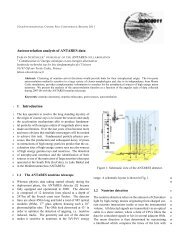
Figure 1.1: The all-particle spectrum from air shower measurements. The shaded area shows
the range of the direct cosmic ray spectrum measurements. Figure taken from [2].
of particle detectors at ground level.
Figure 1.1 shows the measured all-particle spectrum for energies above 10 13 eV. The
flux has been multiplied by E 2.7 in order to display the features of the steep spectrum
that are otherwise difficult to discern.
Above 10 GeV, the flux of the all-particle spectrum is well described by a broken
power-law,
dN
dE 9 E¡γ (1.1)
where N is the number of observed events, E the energy of the primary particle and γ is
the spectral index. The spectral index is about 2.7 up to 3 ¢ 10 15 eV. Above this energy,
the spectral index steepens to about 3.1, introducing the feature known as the knee of the
spectrum. The feature around 10 19 eV is called the ankle of the spectrum and above this
energy the spectral index is again about 2.7.
The change in the slope in the knee region can be explained phenomenologically by
assigning a cutoff energy to the cosmic ray components. This also explains why at around
4 ¢ 10 17 eV, the slope becomes even steeper at the so-called second knee. For relativistic
nuclei with electric charge Ze and energy E in a magnetic field B, the gyroradius is given

12 High Energy Astronomy
by the Larmor radius R L E{ZeB. The propagation of cosmic rays in the Galaxy is
described by the Leaky Box model [3]. In the galactic magnetic field, protons with energy
up to 10 18 eV have a Larmor radius which is smaller than the size of the Galaxy and can
remain confined. Up to these energies, cosmic rays are therefore thought to have a galactic
origin, while at higher energies they can escape from the Galaxy. Heavier nuclei have larger
charges and must therefore be accelerated to larger energies to achieve the same Larmor
radius than protons. Consequently, the heavier element cutoff lies at higher energies and
the composition of cosmic rays for energies above the knee shows a domination of heavier
nuclei over the protons.
Concerning the ankle region, one possible explanation of the flattening of the spectrum
could be the result of higher energy population of particles overtaking a lower energy
population, e.g. an extragalactic flux which starts to dominate over the galactic flux [4].
Furthermore, dimensional analysis related to the Larmor radius and to the fact that, given
the microgauss magnetic field of our Galaxy, no structures are large or massive enough to
reach the energies of the highest energy cosmic rays, limits their sources to extragalactic
objects [5].
1.1.1 The GZK Cutoff
In the highest energy region, not only deflection by the intergalactic magnetic field, but
also the energy losses of cosmic rays in the intergalactic radiation fields, such as microwave,
infrared and radio backgrounds, become important. Soon after the discovery of the Cosmic
Microwave Background radiation (CMB) [6], Greisen [7], Zatsepin and Kuz’min [8]
independently predicted that there would be a cutoff in the spectrum of protons around
6 ¢ 10 19 eV due to photo-production of pions due to interactions with the photons of the
CMB. This phenomenon, known as the GZK cutoff, also limits the possible distance of
any source to several tens of Mpc, the so-called GZK zone.
If cosmic rays are of extragalactic origin, their expected arrival direction distribution
is isotropic for energies below the GZK cutoff. But when their energies exceed the GZK
cutoff energy, the cosmic rays are hardly defected by the intergalactic and/or galactic
magnetic field, and their arrival directions should point back to their sources in the sky, if
the sources are within the GZK zone. Thus a correlation of their arrival directions with the
galactic structure and/or the larger scale of galaxy clusters may be expected [9]. The Pierre
Auger Collaboration reported [10] a correlation of the arrival directions of cosmic rays with
energies exceeding 6 ¢ 10 19 eV with the positions of nearby Active Galactic Nuclei (AGN)
at distances smaller than 75 Mpc. Although this result suggests an anisotropy in the arrival

1.2 Production of Gamma-Rays and Neutrinos 13
Figure 1.2: Expanded view of the high energy end of the cosmic ray spectrum. The most
recent measurements from AGASA [11], HiRes [12] and Auger [13] are shown. Figure taken
from [2].
directions of the cosmic rays, it does not unambiguously identify AGN as the sources of
cosmic rays. Furthermore, it is not confirmed by the other ground-based array experiments
such as HiRes.
Although several experiments have detected cosmic rays above 10 20 eV, the spectral
shape above the ankle is not well determined. The AGASA experiment [11] claimed 11
events above 10 20 eV, while the HiRes [12] and Auger [13] spectra show a significant
steepening of the cosmic ray spectrum above 4 ¢ 10 19 eV, which is consistent with the
prediction of the GZK cutoff.
Figure 1.2 gives an expanded view of the high energy end of the spectrum, showing the
results of the three of ground-based experiments. This figure shows the differential flux
multiplied by a power of the energy, a procedure that enables one to see structure in the
spectrum more clearly, but amplifies small systematic differences in energy assignments
into sizable normalization differences.
1.2 Production of Gamma-Rays and Neutrinos
In general, the acceleration of charged particles by astrophysical sources is described by
two models. The model which describes acceleration of electrons is the so-called lep-

14 High Energy Astronomy
tonic model [14]. Acceleration of protons or other nuclei is described by the so-called
hadronic model [5]. An adequate description of the current experimental situation concerning
gamma-rays can be provided by both models [15]. Since neutrinos are only produced
in the hadronic model, only this model will be discussed.
In the hadronic model, high energy neutrinos and gamma-rays are produced in the
decay of pions which are created in collisions of energetic protons with dense matter or
photon fields.
Accelerated protons interact with photons in the surrounding of the cosmic ray emitters
predominantly via the ∆ resonance:
p γ Ñ ∆ Ñ π 0 X (1.2a)
p γ Ñ ∆ Ñ π¨
X
(1.2b)
Protons can also interact with ambient matter (other protons, neutrons and nuclei),
giving rise to the production of charged and neutral mesons:
p p Ñ π 0 X (1.3a)
p
p Ñ π¨
X
(1.3b)
Neutral pions decay into photons (observed at Earth as γ-rays) with a probability of
almost 98.8%:
π 0 Ñ γγ (1.4)
Charged pions decay into neutrinos with almost 100% probability:
π Ñ ν µ µ
ë ν µ ν e e (1.5a)
π ¡ Ñ ν µ µ ¡ ë ν µ ν e e ¡ (1.5b)
Therefore, in the framework of the hadronic model and in the case of transparent
sources, the energy escaping from the sources is distributed between cosmic rays, γ-rays
and neutrinos. A source is referred to as transparent if its size is larger than the proton
mean free path, but smaller than the meson decay length. For these sources, protons have
large probability of interacting once, and most secondary mesons can decay.
Since the cosmic ray acceleration mechanism also produces neutrinos and high energy
photons, γ-ray sources are in general also candidates for neutrino sources. In the hadronic

1.3 Origin of the Bulk of Cosmic Rays 15
model, the spectral indices of the cosmic ray energy spectrum and the γ-ray and neutrino
spectra are related. It is expected [16] that for nearby sources, they are almost identical.
Hence, γ-ray measurements provide crucial information about primary cosmic rays, and
they constrain the expected neutrino flux.
1.3 Origin of the Bulk of Cosmic Rays
After one century of research, the question of the origin of cosmic rays continues to be
regarded as an unsolved problem. Although the general aspects of the origin of cosmic rays
are considered fairly well-understood, major gaps and uncertainties remain. In general, the
level of uncertainty increases with the cosmic ray energy.
One of the difficulties to distinguish among the various possible scenarios is due to
the fact that the cosmic ray nuclei do not travel in straight lines, but are diffused by the
tangled magnetic fields in the Galaxy. Since cosmic rays with energy below 10 20 eV do not
point back to their sources it is impossible to identify the sources in this way. However,
for the majority of the cosmic rays (i.e. those with energy from 1 to 10 5 GeV per nucleon)
many aspects concerning the origin can be understood in terms of shock acceleration and
diffusive propagation in turbulent magnetic fields in the Galaxy.
The presence in the cosmic radiation of a much greater proportion of secondary nuclei
as spallation products of the abundant primary nuclei, implies that cosmic rays travel
distances thousands of times greater than the thickness of the galactic disk during their
lifetime. This suggests diffusion in a containment volume that includes some or all of the
galactic disk. The fact that the amount of matter traversed decreases as energy increases
suggests that the highest energy cosmic rays spend less time in the Galaxy than the lowest
energy ones. It also suggests that cosmic rays are accelerated before most propagation
occurs. If, on the contrary, acceleration and propagation occurred together, one would
expect a constant ratio of secondary/primary cosmic rays.
Nevertheless, acceleration and transport of cosmic rays are expected to be closely
related. In particular, in the shock acceleration model by supernova blast waves, diffusive
scattering of particles by irregularities in the magnetic field plays a crucial role in the
acceleration as well as the propagation process. Moreover, since acceleration occurs as
the supernova remnant expands into the interstellar medium, there is no sharp division
between acceleration and propagation.

16 High Energy Astronomy
1.3.1 Shock Acceleration and Supernova Explosion
The basic idea of the statistic acceleration mechanism is to transfer macroscopic kinetic
energy of moving magnetized plasma to individual charged particles in the medium due
to repeated collisionless scattering (encounters). Although in each individual encounter
the particle may either gain or lose energy, there is an average net gain of energy after
multiple encounters. Thereby the energy particle is increased significantly and the nonthermal
energy distribution characteristic of particle acceleration is achieved.
In the original paper proposed by Fermi in 1949 [17], charged particles collide with
moving clouds of plasma and begin to diffuse by scattering on the irregularities in the
magnetic field. However, this mechanism, nowadays referred to as the second-order Fermi
mechanism, is not a very efficient acceleration process because the average fractional energy
gain is proportional to pu{cq 2 , where u is the relative velocity of the cloud with respect to
the frame in which the cosmic ray ensemble is isotropic, and c is the light speed.
A more efficient version of the Fermi mechanism is realized when encounters of particles
with plane shock fronts are considered. In this case, the average fractional energy gain
of a particle per encounter is of the first order in the relative velocity between the shock
front and the isotropic cosmic ray front. Currently, the ‘standard’ theory of cosmic ray acceleration
– the so-called Diffusive Shock Acceleration Mechanism (DSAM) – is therefore
based on the first-order Fermi acceleration mechanism. An important feature of DSAM is
that particles emerge out of the acceleration site with a characteristic power-law spectrum
with a spectral index that depends only on the shock compression ratio, and not on the
shock velocity.
The ejected material from a supernova explosion moves out through the interstellar
medium in the form of shock waves at which acceleration can occur. The acceleration hypothesis
is motivated by the fact that the power release in supernovae is about 2 ¢ 10 35 W.
The total power required to supply all the galactic cosmic rays is about 5 ¢ 10 33 W. Even
if there are large uncertainties in these numbers, it appears plausible that an efficiency of
few per cent would be enough for supernova blast waves to energize all the galactic cosmic
rays.
The finite lifetime of the supernova blast wave as a strong shock, however, limits the
maximum energy per particle than can be achieved with this mechanism. For a supernova
with a typical size of 5 pc, the maximum energy is about 10 4 GeV per nucleus. Thus,
since the maximum achieved energy is proportional to the charge per nucleus, according
to this acceleration mechanism the cosmic ray composition becomes progressively enriched

1.3 Origin of the Bulk of Cosmic Rays 17
in heavier nuclei as energy increases beyond the knee region.
The case for supernova explosions as the powerhouse for cosmic rays becomes stronger
with the realization that the first-order Fermi acceleration naturally produces a spectrum
of cosmic rays close to what is observed. Nevertheless the measured spectral index (γ 2.7)
is steeper than the source spectrum (γ 2), because of the energy dependence of cosmic
ray diffusion out of the Galaxy, according to their gyromagnetic radii.
The steepening of the spectrum in the knee region is explained by the end-point of
this kind of acceleration mechanism. To conclude, this model explains a large part of the
spectrum observed from the Earth.
1.3.2 Candidate Galactic Neutrino Sources
The operation of second-generation Imaging Air Cherenkov Technique (IACT) Telescopes,
such as H.E.S.S. [18], VERITAS [19] and MAGIC [20], disclosed the very high energy
gamma-ray sky, revealing a large number of TeV γ-ray sources. Galactic TeV sources
are mainly associated with SuperNova Remnants (SNRs) and X-Ray Binaries, as well
as and with their jetty subclasses: Pulsar Wind Nebulae (PWN) and microquasars [21].
In particular, SNRs and microquasars show peculiar TeV γ-ray emissions that suggest
interactions of accelerated protons on dense media or local radiation fields, that could also
produce TeV neutrino fluxes [22].
A phenomenological approach [23] determines the cosmic ray flux accelerated by SNRs,
required to produce the observed TeV γ-ray flux in the hadronic scenario. In this approach,
interactions between cosmic ray protons and ambient hydrogen clouds result in the production
of mesons which subsequently decay producing photons and neutrinos. Since both
γ-ray and neutrino fluxes depend linearly on the flux of primary cosmic rays, there is also
a linear relation between the γ-ray and the neutrino flux (with a factor of about 2 for
neutrinos, as the photo-production of pions gives the same amounts of π , π ¡ and π 0 ).
If the energy content of the galactic microquasar jets is dominated by electron-proton
plasma, there is the possibility [24] that protons, accelerated at energies larger than
100 TeV by internal shocks within the microquasar jets themselves, could produce TeV
neutrino fluxes through photo-meson interactions with ambient X-ray radiation. Depending
on source parameters, the expected neutrino flux range [25] is Φ ν 10 ¡12 £ 10 ¡10
TeV ¡1 cm ¡2 s ¡1 sr ¡1 .

18 High Energy Astronomy
1.4 Origin of Ultra High Energy Cosmic Rays
The simplest set of assumptions for particle acceleration in the form of DSAM (§ 1.3.1) does
not disclose the origin of cosmic rays with energies greater than roughly 10 17 eV. For these
Ultra High Energy Cosmic Rays (UHECRs), one has to invoke shocks on larger scales,
namely extragalactic shocks. This acceleration scenario is referred to as the bottom-up
scenario. In order to trivially solve the problem of maximum energy achievable, a nonacceleration
mechanism is also possible, referred to as the top-down decay scenario.
In the bottom-up scenario, charged particles are accelerated from lower energies to the
required energies in certain special astrophysical environments. Examples are acceleration
in shocks associated with SNRs, AGN, powerful radio-galaxies, and so on, or acceleration
in the strong electric fields generated by rotating neutron stars with high surface magnetic
fields. On the other hand, in the top-down scenario energetic particles simply arise from
the decay of certain sufficiently massive particles originating from physical processes in
the early Universe, and no acceleration mechanism is invoked at all.
1.4.1 Acceleration Scenarios and Source Candidates
In one possible bottom-up scenario, the supernova blast wave mechanism itself may actually
give energies higher than 10 17 eV. Particles could be accelerated by interactions
with multiple SNRs as they move through the interstellar medium. Moreover, supernovae
probably do not occur in the average interstellar medium. A notable example is Supernova
1987A, which exploded into an environment formed by the wind of its progenitor. This
could raise the maximum energy limit by one or two orders of magnitude [26].
Irrespective of the acceleration mechanism taken into account, a simple dimensional
argument was given by Hillas [27], which allows one to restrict attention to only a few
classes of astrophysical objects as possible sources capable of accelerating particles to a
given energy. In any acceleration scenario, there must be a magnetic field B to keep the
particles confined within the acceleration site. Thus, the size R of the acceleration region
must be larger than the diameter of the orbit of the particle. This argument shows that to
achieve a given maximum energy, the acceleration site must have either a large magnetic
field or a large size (Figure 1.3). Thus, only a few astrophysical sources such as AGN,
radio-galaxies and pulsars satisfy the conditions necessary for acceleration up to 10 20 eV.
Estimates of the typical values of R and B for the central regions of AGN give
R 0.02 pc and B 5 G. These values yield a cutoff energy of approximately 10 19 eV for
protons. However, the energy of accelerated protons is severely degraded due to the photo-

1.4 Origin of Ultra High Energy Cosmic Rays 19
Figure 1.3: Hillas Diagram: Theoretical upper limits of the energy of the particle are determined
by the size and strength of celestial objects.
pion production in interactions with the intense radiation field in and around the central
engine of the AGN. In addition, there are energy losses due to synchrotron and Compton
processes. So neither protons nor heavy nuclei are likely to escape from the central regions
of AGN with such extremely high energies. Nevertheless, the associated ultrahigh energy
neutrinos from the pion decay can escape from AGN cores. The integrated contribution
from all AGN may then produce a diffuse high energy neutrino flux that may be detectable
with a neutrino telescope [28].
The only way to detect this diffuse flux of high energy neutrinos is to look for an
excess of high energy events in the measured energy spectrum induced by atmospheric
neutrinos. It has been pointed out by Waxman and Bahcall [29] that a comparison from
the observations of the diffuse flux of γ-rays and UHECRs leads to an upper bound on
the diffuse neutrino flux of
Eν 2 Φ ν 4.5 ¢ 10 ¡8 GeV cm ¡2 s ¡1 sr ¡1 (1.6)
More details about the Waxman-Bahcall upper limit are given in § 5.2.
Other promising acceleration sites for UHECRs [30] are the so-called hot-spots of

20 High Energy Astronomy
Fanaroff-Riley type II radio-galaxies [31]. The hot-spot is interpreted as a gigantic shock
wave injected by jets emanating from a central active galactic nucleus at relativistic speeds.
The energy loss due to photo-pion production at the source is not significant at hotspots
because the density of the ambient soft photons is thought to be relatively small.
Depending on the magnetic field strength, a maximum energy of up to 10 21 eV seems
to be possible. However, it seems difficult to invoke the radio-galaxies as sources of the
observed Extremely High Energy Cosmic Rays (EHECRs) above 10 20 eV, due to their
large cosmological distances (¡ 100 Mpc) from Earth and the GZK effect.
Acceleration to extremely high energy near the event horizons of spinning supermassive
black holes associated with presently inactive quasar remnants has been suggested by Boldt
and Ghosh [32]. The required effective electromotive force would be generated by blackhole-induced
rotation of externally supplied magnetic field lines threading the horizon.
Another type of sources are gamma-ray bursts (GRBs) which are very short, typically
tens of seconds long, intense flashes of MeV gamma-rays. Various models have been
proposed in order to describe what causes these apparent explosions and which processes
take place during the explosion that leads to the observations. A comprehensive review
is reported in [33]. On the basis of energetics and dynamical considerations, GRBs were
suggested to be UHECR sources [34] via a Fermi mechanism occurring in internal shocks.
GRBs are expected to emit neutrinos during several stages of their evolution [35].
Since GRB neutrino events are correlated both in time and in direction with γ-rays, their
detection is practically background free. A neutrino telescope, triggered by satellite alerts,
could therefore detect them.
Other candidates, motivated by radio observations, are starburst galaxies, common
throughout the Universe, where an exceptionally high rate of star formation has been observed.
The high rate of supernova explosions expected in these regions could enrich the
ambient gas with highly relativistic electrons and protons that interact with the interstellar
medium. Such hidden accelerators of cosmic rays could represent pure high energy neutrino
injectors. A cumulative flux of Eν 2 Φ ν 2 ¢ 10 ¡8¨0.5 GeV cm ¡2 s ¡1 sr ¡1 has been
calculated [36], in agreement with the Waxman-Bahcall upper limit (Eq. 1.6).
1.4.2 Decay Scenario
As previously mentioned, the shock acceleration mechanism is a self-limiting process: For
any given set of values of the acceleration region size R and the magnetic field strength B,
simple criterion of Larmor containment of a particle of charge Ze within the acceleration
region implies that there is a maximum energy E ZeBR up to which the particle can

1.4 Origin of Ultra High Energy Cosmic Rays 21
be accelerated before escaping from the acceleration region.
Because of this difficulty, there is the possibility that the extremely high energy events
may represent a fundamentally different component of cosmic rays in the sense that
these particles may not be produced by any acceleration mechanism at all. These particles
may simply be the result of the decay of some supermassive X particles with mass
m X " 10 20 eV originating from extremely high energy processes in the early Universe. The
sources of the massive X particles could be topological defects such as cosmic strings or
magnetic monopoles that could be formed in the symmetry-breaking phase transitions associated
with Grand Unified Theories at the end of inflation. Alternatively, the X particles
could be certain supermassive metastable relic particles of lifetime comparable to or larger
than the age of the Universe, which could be produced in the early Universe through, for
instance, particle production processes associated with inflation. A comprehensive review
of the top-down scenario can be found, e.g., in [37]. It has to be remarked that mounting
observations pointing out protons as the dominant particles for the EHECRs do not
necessarily rule out superheavy particles as the sources of the highest energy cosmic rays.
Extremely high energy neutrinos are also predicted in a wide variety of top-down
scenarios invoked to produce EHECRs. There are several ways neutrinos can be produced
in the fragmentation of ultra high energy jets. The X particles can decay into quarks,
gluons and leptons [38], which ultimate materialize into, among other particles, nucleons,
γ-rays and neutrinos with energies up to m X . Consequently, besides the photo-production
of pions and subsequent muon decay, neutrinos can be produced by heavy quark decays.
Bottom and charm quarks decay semileptonically about 10% of the time. Furthermore,
top quarks produced in the jets decay nearly 100% of the time to bW ¨. The W -bosons
then decay semileptonically approximately 10% of the time to each neutrino species. In
this scenario, the neutrino flux greatly exceeds the proton flux at energies larger than
10 20 eV.
In the Z-burst scenario [39], ultrahigh energy neutrinos could be the sources of the
GZK air showers. In this scenario, cosmic neutrinos will annihilate on the non-relativistic
relic antineutrinos (and viceversa) at the Z resonance. The Z-boson decays hadronically
about 70% of the time, creating a so-called Z-burst which contains photons and nucleons
with energy near or above the GZK cutoff energy of roughly 5 ¢ 10 19 eV. If the Z-burst
points in the direction of the Earth and it occurs within the GZK distance of Earth
( 100 Mpc), the photons and the nucleons produced by the Z-boson decay may easily
initiate a super-GZK air shower at Earth.
Diffuse high energy neutrino flux measurements and the search for super-PeV neutrinos

22 High Energy Astronomy
can be used to constrain the top-down scenario.
1.4.3 Cosmogenic Neutrinos
In addition to neutrinos generated by high energy cosmic accelerators, there are high
energy neutrinos induced by the propagation of cosmic rays in the local Universe after
their interaction with the CMB [40]. The subsequent pion decay will produce a flux of
so-called GZK or cosmogenic neutrinos. Since neutrinos carry approximately 5% of the
proton energy, this flux is similar to the Waxman-Bahcall bound above 5 ¢ 10 18 eV [41].
In general, about 1% of cosmogenic neutrinos from the UHECR flux is expected.
The detection of these neutrinos will test the hypothesis that the UHECRs are protons
(or possibly somewhat heavier nuclei) of extragalactic origin. On the other hand, an
absence of the GKZ cutoff would reflect into an absence of cosmogenic neutrinos.

Chapter 2
The ANTARES neutrino telescope
A high energy neutrino detector behaves like a telescope when the neutrino direction is
reconstructed with an angular precision of 1 degree or better. This is the case for high
energy charged current muon neutrino interactions. The accurate measurement of the
(anti)muon neutrino direction permits the association with (known) sources. It also allows
the neutrino telescopes to face some of the most fundamental questions in high energy
physics beyond the Standard Model: the nature of Dark Matter through the indirect search
for weakly interacting massive particles (WIMPs); the study of sub-dominant effects of
neutrino oscillations and the violation of Lorentz invariance; the study of relic particles
such as magnetic monopoles or nuclearites in cosmic radiation; the coincident emission of
neutrinos and gravitational waves.
A neutrino telescope is basically a three-dimensional set of arrays of photomultipliers
designed to collect the Cherenkov light (§ 2.1) emitted by neutrino interaction products.
The information provided by the number of photons detected and their arrival times is
used to infer the neutrino track direction and energy.
The ANTARES (Astronomy with a Neutrino Telescope and Abyss environmental Research)
is currently the most sensitive high energy neutrino observatory studying the
Southern Hemisphere including the particularly interesting region of the Galactic Center.
The ANTARES field of view has a sky coverage of 3.5π sr. ANTARES is also a unique
deep-sea marine observatory providing continuous high-bandwidth monitoring of a variety
of sensors dedicated to acoustic, oceanographic and Earth science studies.
The ANTARES Collaboration currently comprises 29 particle physics, astrophysics
and sea science institutes from seven countries (France, Germany, Italy, the Netherlands,
Romania, Russia and Spain).

24 The ANTARES neutrino telescope
Figure 2.1: Schematic view of the production of Cherenkov radiation by a relativistic charged
particle.
2.1 Cherenkov Radiation
Cherenkov radiation [42] is created when a charged particle passes through a medium with
a speed larger than the speed of light in the medium. In this situation, the charged particle
infers a polarization of the molecules along its trajectory. When the dipoles induced by
the polarization restore themselves to equilibrium, a coherent radiation is emitted in a
cone (Figure 2.1).
The angle of the Cherenkov cone depends on the refraction index n of the medium and
the speed v βc of the particle, and can be geometrically calculated. During a time t, the
particle will travel a distance d v βct, while the light will travel a distance d c pc{nqt.
The ratio between d c and d v determines the Cherenkov angle θ C :
cos θ C 1
βn
(2.1)
As high energy neutrinos are relativistic particles (β 1) and the refraction index of sea
water is n 1.364, the Cherenkov angle in sea water is θ C 43 ¥ .
The number of Cherenkov photons N emitted by a particle with unit charge per unit
distance x and unit wavelength λ is [43]
d 2 N
dx dλ 2πα ¢
λ 2 1 ¡ 1
β 2 n 2
(2.2)
where α is the fine-structure constant. Hence a relativistic muon in water emits about
3.5 ¢ 10 4 Cherenkov photons per meter in the 300 – 600 nm wavelength range.

2.2 Detector Layout 25
Mediterranean Sea water
λ 473 nm λ 375 nm
absorption length 60 ¨ 10 m 26 ¨ 3 m
effective scattering length 270 ¨ 30 m 120 ¨ 10 m
Table 2.1: Light propagation parameters for Mediterranean Sea water.
The group velocity of Cherenkov light in a medium v g depends not only on the photon
wavelength and the refractive index of the medium, but also on the wavelength dependence
of the refractive index:
v g c n
¢
1
λ dn
n dλ
c
n g
(2.3)
where n g is the group refractive index of the medium and c is the speed of light. In sea
water in particular, for photons with a wavelength of 460 nm, the group refractive index
is approximately 1.38.
Propagation of light through a medium is governed by absorption and scattering. The
first effect reduces the intensity of the Cherenkov light emitted by the charged particle;
the second effect influences the direction of the Cherenkov photons. Both phenomena
depend on the photon frequency. Photon absorption is characterized by the absorption
length λ abs of the medium, defined as the average distance at which a fraction of e ¡1
of the photons is unabsorbed. Photon scattering in a medium is characterized by the
scattering length λ scat of the medium defined similarly as λ abs , and by the mean scattering
angle xθ scat y. These quantities can be combined into an effective scattering length
λ eff
scat λ scat {p1 ¡ xcos θ scat yq, where xcos θ scat y is the mean cosine of the scattering angle.
The light propagation parameters for Mediterranean Sea water for photons with different
wavelengths are summarized in Table 2.1.
2.2 Detector Layout
The ANTARES detector [44] is located at a depth of 2.475 km in the Mediterranean Sea,
south-east off the coast from Toulon, France (Figure 2.2). An electro-optical cable of about
40 km length serves as the power and data transmission line between the detector and the
ANTARES control room in La Seyne-sur-Mer.
ANTARES is equipped with 885 photomultipliers (PMTs), arranged in triplets on
12 flexible vertical strings.
The basic element is the Optical Module (OM) [46], as shown in Figure 2.3. Each OM
consists of a pressure-resistant glass sphere with a diameter of 43 cm and 15 mm thickness,

26 The ANTARES neutrino telescope
Figure 2.2: The ANTARES detector is located at a depth of 2475 m in the Mediterranean
Sea, about 40 km offshore from Toulon, France (42 ¥ 48’N, 6 ¥ 10’E). Satellite picture taken from
Google Maps [45].
that contains a Hamamatsu R7081-20 PMT. The Hamamatsu R7081-20 is a hemispherical
PMT with a diameter of 25 cm and an effective sensitive area of about 440 cm 2 . It contains
14 amplification stages and has a nominal gain of 5 ¢ 10 7 at a high voltage of 1760 V.
The PMT is sensitive to single photons in the 300 – 600 nm wavelength range; the peak
quantum efficiency is about 25% between 350 and 450 nm. The charge resolution and the
Transit Time Spread (TTS) of the PMT with respect to a single photon are approximately
40% and about 1.3 ns respectively. The dark count rate at the 0.25 photoelectron level is
about 2 kHz. The PMT is surrounded by a µ-metal cage to minimize the influence of the
magnetic field of the Earth on its response. The high voltage is provided by the electronics
board mounted on the PMT socket, which also contains a LED calibration system. A
transparent silicon rubber gel provides the optical and mechanical contact between the
PMT and the glass. The glass hemisphere behind the PMT is painted black and contains
a penetrator which provides the power and data transmission connection to the outside.
The OMs are grouped in triplets to form a storey or floor, as shown in Figure 2.4. They
are mounted at equidistant angles around a titanium Optical Module Frame (OMF), and
point downwards at 45 ¥ with respect to the vertical. The OMs are connected to the Local
Control Module (LCM). The titanium cylinder at the center of the OMF houses the data
transmission electronics of the OMs, as well as various instruments for calibration and
monitoring. A storey may also contain extra instruments that are mounted on the OMF,

2.2 Detector Layout 27
Figure 2.3: Schematic view (left) and picture (right) of an ANTARES optical module.
Figure 2.4: Schematic view (left) and picture (right) of an ANTARES storey.
such as a LED beacon or an acoustic hydrophone.
Storeys are serially connected with Electro-Mechanical Cables (EMCs), which contain
electrical wires for power distribution and optical fibres for data transmission. The distance
between adjacent storeys is 14.5 m. Five storeys linked together constitute a sector, an
individual unit in terms of power supply and data transmission. In each sector, one of the
five LCMs is a Master LCM (MLCM). The data distribution between all LCMs in the

28 The ANTARES neutrino telescope
Figure 2.5: Schematic view of the ANTARES layout.
sector and the String Control Module is handled by the MLCM.
Five sectors linked together form an individual detector line. Each line is anchored to
the seabed by a Bottom String Socket (BSS) and kept vertical by a buoy at the top of
the line and by the buoyancy of the individual OMs. A string is 480 m long, since roughly
100 m from the seabed are left empty to allow for the development of the Cherenkov
cone for upward going particles. The BSS contains a String Control Module (SCM), a
String Power Module (SPM), calibration instruments and an acoustic release system. The
acoustic release allows for the recovery of the complete detector line including BSS except
for a dead-weight. The SPM houses the individual power supplies for all five sectors in
the line. The SCM contains data transmission electronics to distribute data between each
sector and the onshore control room.
The complete detector consists of 12 detector lines in a octagonal configuration, plus a
dedicated instrumentation line (IL), as shown in Figures 2.5 and 2.6. The IL and the top
sector of Line 12 do not contain OMs. Instead, they are equipped with various instruments
for acoustic neutrino detection and for monitoring of environmental parameters. The av-

2.3 Detector Status 29
Figure 2.6: Schematic view of
the ANTARES detector, as seen
from above.
Figure 2.7: Fingerprints of ANTARES.
erage horizontal distance between lines is approximately 60 m. The BSS of each line is
connected to the Junction Box (JB), which is the distribution point of power and data
between the detector lines and the 40 km long Main Electro-Optical Cable (MEOC) to
the onshore control room in La Seyne-sur-Mer.
Figure 2.7 shows x and y coordinates of track fits at the time of the first triggered
hit (§ 2.4.3). The track fits are dominated by downward going atmospheric muons or
muon bundles. The structure of the detector becomes visible because the efficiency of the
trigger algorithm is higher for tracks that pass closer to a detector line. For comparison,
the x and y coordinates of the ANTARES lines are shown in Figure 2.6.
2.3 Detector Status
The ANTARES detector has been fully operational since May 28 th 2008. Prior to its
completion, ANTARES has taken data in intermediate configurations. An overview is
given in Table 2.2. Data taking started in 2006 with the connection of Line 1 on March 2 nd
and Line 2 on September 21 st . On January 29 th 2007, after the connection of Lines 3 – 5,
ANTARES surpassed the Baikal telescope as the largest neutrino telescope on the Northern
Hemisphere. The detector doubled in size on December 7 th 2007 with the connection of
Lines 6 – 10 and the IL. Finally, ANTARES was completed on May 28 th 2008 with the
connection of Lines 11 and 12. Detector lines which showed significant problems during
operation have been recovered, repaired, redeployed and reconnected as shown in the table.
The detector was not operational between June 25 th and September 5 th 2008 due to a fault
in the Main Electro-Optical Cable (MEOC).

30 The ANTARES neutrino telescope
Detector line Connection date Not operational
Line 1 March 2 nd 2006
Line 2 September 21 st 2006
Line 3 January 29 th 2007
Line 4 January 29 th 2007 March 3 rd 2008 – May 28 th 2008
Line 5 January 29 th 2007
Line 6 December 7 th 2007 October 27 th 2009 – present
Line 7 December 7 th 2007
Line 8 December 7 th 2007
Line 9 December 7 th 2007 July 2 nd 2009 – present
Line 10 December 7 th 2007 January 7 th 2009 – November 6 th 2009
Line 11 May 28 th 2008
Line 12 May 28 th 2008 March 12 th 2009 – November 14 th 2009
IL December 7 th 2007
Table 2.2: Operational timeline of the ANTARES detector. The entire detector was not
operational between June 25 th and September 5 th 2008 due to a fault in the MEOC.
2.4 Detector Acquisition
The transport of data and control signals between the PMTs and the onshore control room
and vice versa is handled by the Data AcQuisition (DAQ) system [47]. The DAQ system
involves several steps, such as the signal digitization, the data transmission and the data
filtering and storage.
2.4.1 Signal Digitization
A photon that hits the photo-cathode of a PMT can induce an electrical signal on the
anode of the PMT. The probability for this to happen is characterized by the quantum
efficiency of the PMT. If the amplitude of the signal exceeds a certain voltage threshold,
the signal is read out and digitized by a custom designed front-end chip, the Analogue
Ring Sampler (ARS), located in the LCM. The voltage threshold is set to a fraction of
the single photoelectron average amplitude to suppress the PMT dark current, typically
0.3 photoelectrons. The time the signal crosses the threshold is timestamped by the ARS
with respect to a reference time, provided by a local clock. All clocks in the detector are
synchronized with a 20 MHz onshore master clock. A Time-to-Voltage Converter (TVC)
is used to measure the time of the signal within the 50 ns interval between two subsequent
clock pulses. The TVC provides a voltage which is digitized with an 8-bit Analogue-to-
Digital Converter (ADC) to achieve a timestamp accuracy of about 0.2 ns. Each ARS
contains two TVCs which operate in flip-flop mode to eliminate electronic dead-time. Ad-

2.4 Detector Acquisition 31
ditionally, the charge of the analogue signal is integrated and digitized by the ARS over
a certain time period by using an Analogue-to-Voltage Converter (AVC). The integration
gate is typically set to 35 ns to integrate most of the PMT signal and to limit the contribution
from electronic noise. The combined time and charge information of a digitized
PMT signal is called a hit, and amount to 6 bits. Each PMT is read out by two alternately
operating ARS chips to minimize electronic dead-time. All 6 ARS chips in an LCM
are read out by a Field Programmable Gate Array (FPGA). The FPGA arranges the hits
produced in a certain time window into so-called dataframes, and buffers these dataframes
in a 64 MB Synchronous Dynamic Random Access Memory (SDRAM). The length of the
time window is set to a value much larger than the time it takes for a muon to traverse
the complete detector, typically 13.1072 ms (2 19 ¢ 25 ns) or 104.8576 ms (2 22 ¢ 25 ns).
2.4.2 Data Transmission
Each LCM contains a Central Processing Unit (CPU) which is connected to the onshore
computer system. Each CPU runs two programs that manage the data transfer to shore.
The DaqHarness program handles the transfer of dataframes from the SDRAM to the
onshore control room. The ScHarness program handles the transfer of calibration and
monitoring data, referred to as slow control data. Communication between all offshore
CPUs and the onshore control room is done via optical fibers using the Transmission
Control Protocol and Internet Protocol (TCP/IP). Each LCM CPU in a sector is connected
via a bi-directional Fast Ethernet link (100 Mb/s) and an electro-optical converter
to the MLCM. In the MLCM, these links are electro-optically converted and passed to
an electronic data router (switch). The switch merges the 5 bi-directional Fast Ethernet
links (4 LCM and 1 MLCM CPU) into two uni-directional Gigabit Ethernet links
(1 Gb/s), one for incoming control signals and one for outgoing data. The gigabit signals
are electro-optically converted using an optical wavelength which is unique for each
MLCM in a detector line. The incoming and outgoing optical links of the 5 MLCMs in
a detector line are routed to the String Control Module, where they are (de)multiplexed
into a single optical fiber using Dense Wavelength-Division Multiplexing (DWDM). The
optical fiber from each String Control Module runs through the Junction Box and the
Main Electro-Optical Cable to the onshore control room, where they are (de)multiplexed
into separate MLCM channels using the same wavelengths as in a detector line. The unidirectional
optical MLCM channels from all demultiplexers are linked to an onshore switch
via electro-optical converters. Finally, the switch is connected to a computer farm which
accommodates the detector control and the data processing systems.

32 The ANTARES neutrino telescope
2.4.3 Data filtering and storage
The DAQ system is designed according to the so-called All-Data-To-Shore concept. This
concept entails that no offshore signal selection is done except for the ARS threshold
criterion, and all detected hits are transferred to shore. However, since the vast majority
of detected signals is due to the optical background in the detector (§ 2.6), the data are
filtered in the onshore computing farm to reduce the data storage demands. This is done
by sending all dataframes that belong to the same time window to a common processor
in the onshore computer farm. The complete set of dataframes from all ARS chips in the
detector that correspond to the same time window is referred to as a timeslice, which
consequently contains all hits that were detected in the same time window. Each timeslice
is handled by a different processor, each of which accommodates a dfilter program. The
dfilter program collects all dataframes corresponding to the same timeslice, and applies
a trigger algorithm to search for signals that can be attributed to a charged particle which
traversed the detector. Hence data filtering is done using software rather than hardware,
which has advantages in terms of flexibility and detection sensitivity. Different trigger
algorithms can be applied in parallel to search for specific signatures. The output from
every datafilter is passed to the dwriter program that formats the data using the ROOT
software package [48] and stores them in a database for offline analysis. Similarly, the slow
control data are collected and processed by the scDataPolling program, and written to
the database by the dbwriter program.
2.5 Detector Calibration
The precision with which the direction and energy of charged particles which traverse the
detector can be determined, depends on the accuracy with which the photon arrival times
at the PMTs and the location of those PMTs are measured. ANTARES is designed to
achieve an angular resolution smaller than 0.3 ¥ for muons above 10 TeV [49]. To realize
this resolution, the ANTARES detector comprises several independent calibration systems
that are able to measure and monitor the absolute and relative timing of PMT signals and
the location of all PMTs.
2.5.1 Time Calibration
The relative timing of the photon arrival times on the PMTs are needed to reconstruct the
neutrino direction. Hence the offset of each local clock, caused by the optical path length
to shore, has to be known. The offsets are obtained by an internal clock calibration system.

2.5 Detector Calibration 33
A calibration signal sent by the onshore master clock is echoed back along the same optical
path by each LCM, to measure the relative offset of each LCM with an accuracy of 0.1 ns.
A second calibration system based on a blue (470 nm) LED inside each OM is used to
calibrate the time offset between the PMT photo-cathode up to the read-out electronics.
The internal LED system is used in dedicated data-taking runs to monitor the relative
variation of the PMT transit time. Finally, a calibration system based on optical beacons
in the detector is used to calibrate the relative time offsets between PMTs. The system
comprises four blue (472 nm) LED beacons located on storeys 2, 9, 15 and 21 of each
detector line, and two green (592 nm) LASER beacons on the BSS of Lines 7 and 8. A
small PMT in each LED beacon and a photo-diode in each LASER beacon measure the
time of emission. Dedicated data-taking runs in which one or several beacons are flashed
are performed regularly (typically once per week), to monitor the relative time offsets
between the PMTs and the influence of water on the light propagation.
Measurements obtained by the internal LED and optical beacon systems have shown
that the contribution of the detector electronics to the photon arrival time resolution
is less than 0.5 ns [49]. Therefore the time resolution is dominated by the TTS of the
PMTs (σ TTS 1.3 ns), and the light scattering and chromatic dispersion by the sea
water (σ sea 1.5 ns, for an optical path length of 40 m).
The presence of 40 K (§ 2.6) in the sea water provides a convenient calibration source,
which is used to verify the time offsets between the triplet of PMTs within a storey, as well
as the long term stability of the PMT efficiencies. A mean coincidence rate of 16 ¨ 2 Hz
has been observed. This agrees with the expected rate of 19 ¨ 3 Hz, obtained by Monte
Carlo simulations [50].
Absolute timing is needed to correlate the reconstructed neutrino direction with specific
sources in the Universe. This is achieved by synchronizing the onshore master clock to the
Global Positioning System (GPS) time with an accuracy of 100 ns [47].
2.5.2 Charge Calibration
The charge calibration and threshold tuning of the PMTs and their associated frontend
electronics enables to translate signal amplitudes into units of number of photoelectrons
(p.e.), which are used in the track and energy reconstruction.
All the ARSs (§ 2.4.1) have been calibrated prior to deployment, measuring the transfer
functions of the Analogue-to-Voltage Converter (AVC). This AVC transfer function is an
important parameter for the correction of the so-called walk of the PMT signal, and for
the measurement of the amplitude of each PMT pulse. The principal component used in

34 The ANTARES neutrino telescope
the on-shore calibration procedure is a pulse generator which directly sends signals to a
pair of ARSs operating in a flip-flop mode. The generated pulse has a triangular shape
with 4 ns rise time and 14 ns fall time, somewhat similar to the electrical pulse of a PMT
with variable amplitude. The transfer functions of the dynamic range of the AVCs are
linear and can therefore be parameterized by their slope and intercept. The distributions
of these two parameters for a large sample of ARS chips have demonstrated that they are
homogenous [51]. This implies that the same parameters can be used for all ARSs.
After the deployment, special data-taking runs reading the PMT current at random
times enable the measurement of the so-called pedestal value of the AVC channel. The
single photoelectron peak can be studied using randomly triggered events, since the optical
activity due the 40 K decays and bioluminescent bacteria (§ 2.6) produces, on average,
single photons at the photo-cathode level. The knowledge of the photoelectron peak and
the pedestal is used to estimate the charge over the full dynamical range of the AVC. The
AVC channel values of the pedestal and the single photoelectron peak are used to convert
the analogue charge measurements of the PMT signals into photoelectron units.
Furthermore, since the 40 K coincidence rate is constant, it can be used to monitor the
time evolution of the detector response. The 40 K coincidence rate has shown a regular
decrease indicating a gain decrease of the PMTs. The PMT gain drop is thought to be
due to ageing of the photo-cathode. Indeed, after the period between July and September
2008 when the detector was off for cable repair, the gains seem to have partially recovered
when the PMTs were switched off [51].
2.5.3 Position Calibration
Each detector line is anchored to a BSS on the seabed and kept vertical by the buoyancy
of the individual OMs and a top buoy. Nevertheless, due to the sea current and the
flexibility of the Electro-Mechanical Cables, the radial displacement of a detector line can
be considerable and real time positioning of each line is needed. This is achieved through
two independent systems: an acoustic positioning system and a tiltmeter-compass system.
The acoustic positioning system consists of a three-dimensional array of acoustic
emitters and receivers (hydrophones). The emitters, capable of sending high frequency
(40 – 60 kHz) acoustic signals, are located on the BSS of each line. An additional independent
autonomous emitter is located approximately 145 m from the detector array. Five
hydrophones are located on Storeys 1, 8, 14, 20 and 25 of each detector line. Dedicated
acoustic runs are performed every 2 minutes, during which the transit times between each
emitter and the receivers are recorded. The distances between emitters and receivers are

2.5 Detector Calibration 35
Figure 2.8: The horizontal movements of all hydrophones on Line 10 relative to the bottom
of the line during February 2010; black points represent the hydrophone on Storey 1, red on
Storey 8, blue on Storey 14, green on Storey 20 and magenta on Storey 25.
calculated using the sound velocity which is monitored by several sound velocity profilers
located throughout the detector. The calculated distances are then used to triangulate
the position of each acoustic receiver relative to the acoustic emitters with an accuracy
of 10 cm [52].
The tiltmeter-compass system comprises a tiltmeter and a compass in each LCM. The
two perpendicular tilt angles of a storey, the pitch and roll angles along the North-South
and East-West axes, are monitored by a tiltmeter with an accuracy of 0.2 ¥ . The heading
angle of a storey with respect to the North-South axis is monitored with a compass with
an accuracy of 1 ¥ . The tiltmeter-compass data are also read out every 2 minutes.
The shape of each detector line is reconstructed by performing a global chisquare-like
fit using information from both of these systems. The line shape is used to calculate the
relative position of each PMT in the detector line with respect to the BSS. The absolute
position of the BSS of each line is determined during the connection of a line to the Junction
Box with a Remotely Operated Vehicle (ROV). This is done by acoustic positioning and
water pressure measurements by the ROV, and the GPS location of the ship.
Figure 2.8 shows the movement of various storeys on a line, relative to its center axis.
The extent of the displacement depends on the intensity of the sea current. For typical
currents of few centimeters per second, the displacement is a few meters for the topmost
storeys.

36 The ANTARES neutrino telescope
Figure 2.9: Median rate (in kHz) of measured single photon counts for Line 1 and IL, since
July 2005 until June 2009. The greed, red and blue lines indicate the median counting rates
in storey 1 of the IL, the bottom of Line 1 (Storey 1, OM 1) and the top of Line 1 (Storey 25,
OM 1) respectively.
2.6 Optical Background
Sea water contains two naturally occurring and independent sources of visible light, which
have to be taken into account in neutrino telescopy: the radioactive potassium isotope 40 K
and bioluminescence.
Monitoring of the sea water salinity at the ANTARES shows that it is constant at
about 3.9%. This implies that sea water consists for about 400 ppm of potassium. About
0.012 % of potassium consists of the long-lived radioactive isotope 40 K, which has a halflife
of 1.3 billion years. It can decay to 40 Ca through beta decay (89% of the time) and
to 40 Ar through electron capture and emission of an energetic photon (11 % of the time).
In the beta decay ( 40 K Ñ e ¡ ν 40 e Ca), the maximum electron energy of 1.3 MeV
lies above the Cherenkov threshold in water. In the electron capture ( 40 K e ¡ Ñ 40 Ar*,
followed by 40 Ar* Ñ 40 Ar γ), the photon energy of 1.46 MeV is sufficiently high to
Compton scatter an electron above the Cherenkov threshold. A dedicated Monte Carlo
simulation indicates that the counting rate for each PMT in the ANTARES detector due
to 40 K events is constant at 34 ¨ 7 kHz [53].
The median counting rate per PMT for a number of arbitrary PMTs in ANTARES,
as measured between 2005 and 2009, is shown in Figure 2.9. The corresponding mean
counting rate per PMT, the so-called baseline rate (which on average varies between
60 and 100 kHz), is higher than what is expected from 40 K alone, and is highly time
dependent. It is assumed that the surplus and time variations are due to bioluminescence,
light produced by organisms living in the water. The amount of bioluminescent light
detected in ANTARES is expected to be correlated to the amount of luminescent organisms
in the water, and hence to the sea current velocity. Furthermore, occasionally the baseline

2.6 Optical Background 37
rate increases up to several MHz for short periods of time. These so-called bursts can last
for seconds and are thought to be produced by organisms hitting the PMTs. The fraction
of time during which the instantaneous background rate exceeds the baseline rate by at
least 20% is referred to as the burst fraction.

Chapter 3
Parameterization of Atmospheric
Muons
The most abundant signal seen by a neutrino telescope is due to high energy downward
going muons produced in the extensive air showers resulting from interactions between
primary cosmic rays and atmospheric nuclei. Although the shielding effect of the sea
reduces their flux, at the ANTARES site the atmospheric muon flux is about six orders
of magnitude larger than the atmospheric neutrino flux (Figure 3.1). These atmospheric
muons represent a dangerous background for track reconstruction as their Cherenkov light
can mimic fake upward going tracks. On the other hand, they are a useful tool to test offline
analysis software, to check the understanding of the detector and to estimate systematic
uncertainties.
This chapter starts with a brief description of the interaction of cosmic rays with the
atmospheric nuclei and the subsequent creation and propagation of secondary particles
through the atmosphere (§ 3.1). The primary cosmic ray models used as first inputs in
the Monte Carlo simulations of underwater atmospheric muons are discussed in § 3.2.
Particular interest is given to the HEMAS parameterization [54] from which parametric
formulae [55] have been derived (§ 3.3) and compared to experimental data of some neutrino
telescopes (§ 3.4). These formulae have been subsequently used to develop a fast
event generator, called MUPAGE [56]. This code is one of the main topics of this thesis
and it will be presented in the following chapter.
3.1 Cosmic Ray Interaction with the Earth’s Atmosphere
Cosmic rays with an energy above about 10 12 eV are capable of generating cascade showers
containing thousands of secondary particles through interactions with the atmosphere.

40 Parameterization of Atmospheric Muons
Figure 3.1: Different contributions to muon background as a function of the zenith angle.
Atmospheric muons at a depth of 2 km w.e. are from MUPAGE [56] and atmospheric neutrinoinduced
muons are from calculations by Bartol [57]: The dotted line stands for E ν ¡ 100 GeV
and the dashed-dotted line for E ν ¡ 1 TeV.
During the propagation of the air showers in the atmosphere, the number of particles
initially increases until it reaches a maximum, after which it attenuates as more and more
particles fall below the energy threshold for further particle production (about 1 GeV).
The initial interaction is
CR
N Ñ π¨, π 0 , K¨, K 0 , p, n, . . . , exotic particles
A cosmic-ray-induced air shower can be described by three components: electromagnetic,
muonic and hadronic. The classic discussion by Greisen is reported in [58]. The
shower consists of a core of high energy hadrons that continually feed the electromagnetic
part of the shower, primarily by photons from decay of neutral pions and eta particles.
Each high energy photon generates an electromagnetic subshower through pair production
and bremsstrahlung interactions with the atmosphere. However, as the shower develops,
the number of electrons and positrons declines rapidly after reaching a maximum because
radiation and pair production processes subdivide the energy down to the critical energy
after which electrons quickly lose the remaining energy by ionization. Nucleons and other
high energy hadrons contribute further to the hadronic cascade. Lower energy charged
pions and kaons decay to feed the muonic component.
Below 100 GeV, most pions and kaons produced in the atmosphere decay before they

3.1 Cosmic Ray Interaction with the Earth’s Atmosphere 41
interact. The pion decays (and their branching ratios) are the same decays which produce
astrophysical neutrinos and γ-rays, namely
π Ñ µ ν µ p 100%q (3.1a)
π ¡ Ñ µ ¡ ν µ p 100%q (3.1b)
π 0 Ñ γγ p 98.8%q (3.1c)
Kaons decay with almost 63.5% probability to:
K Ñ µ ν µ (3.2a)
K ¡ Ñ µ ¡ ν µ (3.2b)
These meson decays significantly contribute to the production of atmospheric muon neutrinos.
Another particular important semileptonic decay channel to take into account, with
almost 40.6% of branching ratio, is
KL 0 Ñ π e ¡ ν e (3.3a)
KL 0 Ñ π ¡ e ν e (3.3b)
which is the dominant source of atmospheric electron neutrinos for energies higher than
10 GeV when muon decay is unimportant. Muons indeed are nearly stable and rarely interact
catastrophically, but only lose energy relatively slowly by ionization of the medium.
Therefore, muons give the dominant signal deep in the atmosphere, underground and
underwater.
Production of heavier flavors, especially charm, eventually becomes important for muon
and neutrino fluxes at very high energy. Above 1–10 TeV, the semileptonic decays of very
short-lived charmed particles like D mesons and Λ baryons are the dominant sources,
despite their low production rate. The main contribution comes from the D meson decay
modes, in the charged (almost 9% of probability)
D Ñ K 0 l ν l (3.4a)
D ¡ Ñ K 0 l ¡ ν l (3.4b)
and in the neutral (roughly 3-4% of probability) channels
D 0 Ñ K ¡ l ν l (3.5a)
D 0 Ñ K l ¡ ν l (3.5b)

42 Parameterization of Atmospheric Muons
and from the Λ c baryon decay mode (roughly 2% probability):
Λ c Ñ Λ 0 l ν l (3.6)
where l can be only e or µ.
The role of D s meson decay
D s Ñ l ν l (3.7a)
D s ¡ Ñ l ¡ ν l (3.7b)
is almost negligible (of order to 10 ¡3 ) for the production of e and µ, but has a branching
ratio of almost 7% for the production of τ and ν τ [59].
Because of the short lifetime of these particles, heavy meson and baryon decays are not
inhibited by interactions with the atmosphere for energies below about 10 8 GeV. Muons
and neutrinos generated in heavy flavor decay are called prompt leptons. The energy at
which the contribution of prompt muons to the sea level flux becomes equal to that of
muons from π, K decays is expected to be between 10 TeV and 10 3 TeV, depending on
the charm production model [60].
3.2 Primary Cosmic Ray Models
The two main ingredients that have to enter in the Monte Carlo simulations of atmospheric
muons are the cosmic ray energy spectrum and composition, and the properties of the
inelastic interactions of nucleons with air nuclei. Then, the particles must be propagated
in the atmosphere and in the overburden medium of the detector.
Although the general features of the muon spectrum measured at ground level are well
understood, differences between Monte Carlo computations and experimental data up to
25–30% exist [61]. These differences could reside either in an incorrect knowledge of the
cosmic ray energy spectrum and composition or in the adopted interaction model.
Concerning the cosmic ray composition, different models have been introduced with the
intent of reproducing the cosmic ray energy spectrum behavior for mass group elements. It
is customary in the Monte Carlo computations to account for five mass groups of primaries,
namely H, He, C+N+O, Mg+Si, Fe. This selection follows the fact that these nuclei are
the ones synthesized by nuclear-fusion processes occurring in different stages of massive
star evolution and are subsequently spread out in the Galaxy during supernova explosions.
The most common parameterizations of the primary cosmic rays are: NSU [62], polygonato
[63], HEMAS [54] and FLUKA [64].

3.2 Primary Cosmic Ray Models 43
The HEMAS code was developed to simulate the muon flux underground and it was extensively
used by the MACRO experiment at Gran Sasso (Italy) in the study of the muon
flux and the muon bundle rate [65] at an average depth of 3400 m w.e. Hadronic interactions
in the atmosphere are handled with the hadronic interaction code DPMJET [66]. In
HEMAS, the energy spectrum assumed to generate each mass group is represented by a
function of the form
ΦpEq K i E ¡γ i
(3.8)
where K i and γ i have different values depending on the mass group and E is the energy
per particle. Furthermore, for the same nucleus, they have different values before and after
the knee energy E k . The values of the constants are reported in Table 3.1.
Nucleus Z A K 1 γ 1 K 1 γ 2 E k
[m 2 s sr GeV] ¡1 [m 2 s sr GeV] ¡1 [GeV]
H 1 1 3000 2.56 2.1 ¢ 10 6 3 3 ¢ 10 6
He 2 4 20100 2.74 6 ¢ 10 6 3.12 2 ¢ 10 6
CNO 7 14 600 2.5 3.7 ¢ 10 7 3.24 3 ¢ 10 6
Mg-Si 12 24 877 2.5 6.3 ¢ 10 7 3.25 3 ¢ 10 6
Fe 26 56 311 2.36 4.1 ¢ 10 6 3 2.7 ¢ 10 6
Table 3.1: The constants used in the HEMAS model.
Figure 3.2 shows the comparison of Monte Carlo input spectra, considering the convolution
of the all particle groups (all-particle). The plot represents the differential spectra
multiplied by E 2.7 as a function of energy per particle. The value 2.7 is very close to the
weighted average of the spectral indices of the elements with Z from 1 to 28 deduced by
the best fits to experimental data as presented in [67]: γ Z ¡p2.684 ¨ 0.008q. The ‘theoretical’
spectra will thus appear almost horizontal with a trend to increase (decrease)
according to their spectral indices having values smaller (larger) than the above chosen
value. Moreover, by using a logarithmic scale along the y-axis it is straightforward to appreciate
the percentage deviations of one model from the others, that can vary from 10%
to 100% in absolute value.
The polygonato and the NSU models show the apparent major difference in the shape
of the knee that is much sharper in the former one. The HEMAS parameterization tends
to overestimate the individual spectra and in particular the Fe spectrum with respect to
the other models, as a consequence of a flatter spectral index. However, the knee position
in the all-particle spectrum seems to coincide with that of the polygonato and NSU model.

44 Parameterization of Atmospheric Muons
Figure 3.2: Parameterizations of the all-particle input spectra of Monte Carlo computations
cited in the legend: HEMAS [54], NSU [62], FLUKA [64] and polygonato [63].
The FLUKA model overestimates the contribution of medium nuclei (CNO, Mg-Si and
Fe) by assuming softer spectral indices for their spectra. The effect is that the knee of
the all-particle spectrum is smoother and displaced at a higher energy than in the other
models.
The all-particle spectrum as a function of energy resulting from measurements by some
direct and indirect experiments is shown in Figure 3.3 compared to the Monte Carlo predictions.
As already mentioned, the ‘theoretical’ spectra have been multiplied by E 2.7 and
for comparison so are the experimental data. As a consequence, if the energy normalization
of an experiment is overestimated (underestimated) by a factor κ, the flux intensity
will be overestimated (underestimated) by a factor κ 1.7 . This emphasizes the deviations
between experimental data sets and ‘theoretical’ models.
Although the HEMAS parameterization seems to overestimate the overall flux with
respect to the other parameterizations as well as the observations, it should be remarked
that the observable variables are obtained after the unfolding with the interaction model.
For this reason, HEMAS in combination with the DMPJET interaction model have been
preferred over other models, since they were deeply used and cross-checked with the results
of the underground MACRO experiment. Additionally, the input primary cosmic
ray spectrum is based on a phenomenological model obtained by MACRO [65]. Moreover,
HEMAS is optimized to reproduce the multiplicity distribution of muons in bundles and

3.3 Parametric Formulae of Underwater Muons 45
Figure 3.3: All-particle input spectra deduced by direct (ATIC [68] and RUNJOB [69]) and
indirect (KASKADE [70], DICE [71], CASA-BLANCA [72], TUNKA [73] and Akeno [74])
measurements and the parameterizations used in the Monte Carlo simulations (HEMAS [54],
NSU [62], FLUKA [64] and polygonato [63]).
the lateral distribution of muons inside the bundle at different depths of standard rock.
3.3 From the HEMAS Model to the Parametric Formulae
of Underwater Muons
A parameterization of the multiple muon flux and energy spectra [55] has been deduced
from the results of a full Monte Carlo simulation of the primary cosmic ray flux, interactions
and shower propagation in the atmosphere. The latest version of the HEMAS code
was used: HEMAS-DPM [75].
The reliability of the code is restricted to secondary particles with energies above
500 GeV. Muons that have a lower energy at sea level are discarded because their survival
probability for depths larger than 1.5 km w.e. is very small, and completely negligible at
2 km w.e.
The so-called prompt muons (§ 3.1) and other short-lived particles produced in the
interactions of cosmic rays with the atmosphere are not included in the Monte Carlo simulation.
An unknown uncertainty factor due to these processes should be included for muon
residual energies higher than roughly 10 TeV.

46 Parameterization of Atmospheric Muons
Figure 3.4: Muon energy loss in water from [76]: p = e e ¡ pair production;
b = bremsstrahlung; pn = photo-nuclear interaction; ion = ionization.
3.3.1 Muon Energy Loss in Water
Muons that traverse through matter lose energy by ionization and by radiative processes:
bremsstrahlung, direct production of e e ¡ pairs, and photo-nuclear interactions. In the
ionization process, the muon interacts with the electric field generated by the electron
cloud of the atom. In the radiative processes, the muon interacts with the nuclear electric
field of the atom.
The total muon energy loss may be expressed as a function of the amount of matter
traversed X as [2]
¡ dE µ
dX a bE µ (3.9)
where a is the ionization loss and b is the fractional energy loss by the three radiative
processes. Figure 3.4 shows the energy loss due to different interactions in water as a
function of the muon energy. As can be seen, ionization is nearly independent of energy,
whereas the radiative processes are proportional to the muon energy.
The quantity ɛ a{b defines a critical energy below which continuous ionization loss
is more important than radiative losses.
In the full Monte Carlo simulation, the muons in the atmospheric showers that reached
the sea level were propagated down to 5 km of water using MUSIC [76], a three-dimensional
muon propagation code which uses recent and accurate cross sections of the muon interactions
with matter.

3.3 Parametric Formulae of Underwater Muons 47
Figure 3.5: Flux of muon bundles as function of multiplicity m at depth h 2.5 km w.e. for
five different zenith angles, θ 0 ¥ , 20 ¥ , 40 ¥ , 60 ¥ and 70 ¥ as computed with Eq. (3.10).
3.3.2 Flux of Muon Bundles
The flux of single and multiple muons (so-called muon bundles) with multiplicity m is
obtained as a function of vertical depth h and zenith angle θ [77], using two free parameters
(K and ν), as:
Kph, θq
Φpm, h, θq (3.10)
m νph,θq
The validity range of the vertical depth h is between 1.5 and 5 km w.e., the validity range
of the zenith angle θ is up to 85 degrees.
Figure 3.5 shows how the flux of muon bundles of increasing multiplicity m decreases
with the zenith angle.
3.3.3 Energy Spectrum
Assuming a power-law for the primary beam energy, the expected muon energy distribution,
at a slant depth X h{ cos θ, is described by [78]:
dN
dplog 10 E µ q G ¤ E µe bXp1¡γq rE µ ɛp1 ¡ e ¡bX qs ¡γ (3.11)
where γ is the spectral index of the primary cosmic rays and ɛ is defined from the parameters
of the muon energy loss formula (Eq. 3.9). γ and ɛ are used as free fit parameters
and b is fixed. G Gpγ, ɛq represents a normalization constant so that the integral over
the muon energy spectrum (Eq. 3.11) from 1 GeV to 500 TeV is equal to one.

48 Parameterization of Atmospheric Muons
Figure 3.6: Differential energy spectra (normalized to unit area) of vertical (θ 0 ¥ ) single
muons at different depths (h = 2, 3, 4 and 5 km w.e.). The marker points (superimposed to
h = 2 km w.e.) correspond to the values obtained with the full Monte Carlo simulation. Figure
taken from [55].
Figure 3.6 shows the energy distribution of vertical (θ 0 ¥ ) single muons at various
depths. The energy spectrum is evaluated by multiplying the normalized energy distribution
(Eq. 3.11) with the flux (Eq. 3.10) of vertical single muons: Φ 1 Φpm 1, h, θ 0 ¥ q.
For instance, at h = 3 km w.e., Φ 1 1.6 ¢ 10 ¡4 (m 2 s sr) ¡1 . The total muon flux is
Φ T
° m Φpm, h 3 km w.e., θ 0¥ q 2.2 ¢ 10 ¡4 (m 2 s sr) ¡1 . Note that, as each
integrated energy spectrum is normalized to 1, Eq. (3.11) gives only the shape of the
distribution.
The situation is more complicated for multiple muons. Particles resulting from hadronair
interactions are produced in clusters. The number of charged hadrons follows a negative
binomial distribution, whose characteristic depends on their primary energy. The transverse
momentum p t of the mesons follows in part an exponential-law distribution and in
part a power-law distribution [75, 79]; most of the energy is concentrated in the very forward
region (i.e. near the longitudinal axis). Muons produced in the decay of secondary
mesons which reach a given water depth h follow the energy distribution of the parent
mesons. As a consequence, in a muon bundle, the most energetic muons are expected to
arrive closer to the shower axis. This effect is shown in Figure 3.7, obtained from the Monte

3.3 Parametric Formulae of Underwater Muons 49
Figure 3.7: Differential energy spectra (normalized to unit area) of double muons (m 2)
assuming vertical direction (θ 0 ¥ ) and depth h = 3.5 km w.e., at five different distances from
the bundle axis: R 3, 10, 30, 50 and 70 m. The marker points (superimposed to R = 3 m)
correspond to the values obtained with the full Monte Carlo simulation. Figure taken from [55].
Carlo parameterization in [55] assuming the vertical direction and a depth h 3.5 km w.e.
Hence, the energy spectrum (Eq. 3.11) of muon bundles depend not only on the vertical
depth h and on the zenith angle θ, but also on the muon bundle multiplicity m and on
the muon radial distance R from the shower axis.
3.3.4 Lateral Spread
The muon lateral distribution in a plane perpendicular to the shower axis can be described
as [54]
dN
dR C R
pR R 0 q α (3.12)
where R is the distance from the shower axis and C, R 0 and α are parameterization
constants.
Figure 3.8 shows the normalized lateral distribution of vertical double muons at different
depths h as obtained from Monte Carlo parameterization in [55].
The average distance of all muons in a bundle to the shower axis depends on the bundle
multiplicity m, on the vertical depth h and on the zenith angle θ. At a given depth, the
average distance to the shower axis of each muon in a bundle slightly decreases when the

50 Parameterization of Atmospheric Muons
Figure 3.8: Lateral distribution (normalized to unit area) for vertical double muons (m 2)
at four different depths (h = 2, 3, 4 and 5 km w.e.). Figure taken from [55].
multiplicity m increases. This can be qualitatively understood because bundles with high
multiplicities are generally produced by primary parents of high energies.
3.3.5 Multiplicity
The distribution of the muon multiplicities in a bundle depends on the vertical depth h
and on the zenith angle θ. The dependence of the multiplicity distribution on these two
variables is the following: for a fixed zenith angle θ, bundles with high multiplicity are
suppressed when h increases; for a fixed vertical depth h, bundles with high multiplicity
are suppressed when θ increases (Figure 3.9). In both cases the number of muons in the
bundle decreases because increasing h or θ is equivalent to increasing the path length in
the water through which muons travel.
3.4 Comparison of Parametric Formulae with Experimental
Data
A comparison of the zenith distribution evaluated at a fixed depth using Eq. (3.10) with
some experimental data has been performed [80]. Figure 3.10 shows a comparison between
the predicted muon zenith angular distribution at three different depths and the
measurements of the ANTARES [81] and Baikal [82] underwater neutrino telescopes and

3.4 Comparison of Parametric Formulae with Experimental Data 51
Figure 3.9: Average muon event multiplicity m h as function of the cosine of the zenith angle θ
at the fixed sea depth h = 2 km for energies larger than 20 GeV. Figure taken from [81].
the AMANDA-II [83] under-ice experiment. The AMANDA data (triangular markers)
superimposed to the line at a vertical depth h = 1.68 km w.e. have been converted to
intensities relative to the underwater depths, taking into account the lower ice density
ρ ice = 0.917 g cm ¡2 .
The comparison demonstrates that the analytical solution provides a good represen-
Figure 3.10: Muon flux as a function of the cosine of zenith angle θ as measured by
ANTARES [81], AMANDA-II [83] and Baikal [82] at three different depths. The results obtained
by the parametric formulae at the three depths are superimposed as full lines.

52 Parameterization of Atmospheric Muons
tation of the experimental data so far collected. This is true also in the case of the Baikal
experiment, at a depth h = 1.17 km w.e., nominally outside the range of validity of the parameterization.
Note that not all experiments have declared their systematic uncertainties.

Chapter 4
The Simulation of Underwater
Atmospheric Muons:
the MUPAGE Code
The development of an event generator of atmospheric muons for neutrino telescopes deduced
from the parametric formulae introduced in Chapter 3 is one of the main topics of
this thesis. This chapter describes MUPAGE (MUon GEnerator from PArametric formulae),
a standalone C++ code, already published in [56]. It produces, in an ASCII table,
the muon event kinematics on the surface of the so-called can, an imaginary cylinder surrounding
the active volume of a generic underwater/ice neutrino telescope. The ASCII
table can subsequently be used as input in the following steps of a detector-dependent
Monte Carlo simulation, which includes production of light in water/ice and simulation of
the signal in the detection devices. Some applications of MUPAGE can be found in [84].
§ 4.1 presents the structure of the MUPAGE code. § 4.2 describes the generation of
events on the surface of the can, in which a Hit-or-Miss method [85] is applied. Events
can be single muons (§ 4.3) or the more complex multiple muons (§ 4.4). There is neither
bias nor ordering (in energy, multiplicity and zenith angle) in the simulation. All events
have the same weight, thus the output file reproduces a real data file. For each run the
livetime is computed as described in § 4.5. In § 4.6, using MUPAGE as event generator,
the angular distributions of reconstructed atmospheric muon tracks have been computed
and subsequently compared with the ANTARES data.
4.1 Program Structure
MUPAGE needs some input parameters, as described in [56], such as the detector configuration
(Figure 4.1), the density of the detector medium and the ranges of the various

54 The Simulation of Underwater Atmospheric Muons: MUPAGE
Figure 4.1: Sketch of the geometrical meaning of some input parameters. The cylinder surrounding
the instrumented volume is the can, with radius R can and height H can . The events
are generated on an extended can, with R ext R can R ecr [56]. The lower disk is at a depth
H max with respect to the sea/ice surface. The origin of the detector coordinate system lies on
the cylinder axis, but it does not necessarily coincide with the center of the cylinder.
simulation parameters (e.g. multiplicity, zenith angle, muon energy).
As shown in Figure 4.1, the radius of the generation volume must be increased by
a quantity R ecr , in order to accept peripheral muons in large bundles. These peripheral
muons are due to the high multiplicities of bundles (which at roughly 2 km w.e. depth can
reach up to 10 3 muons per bundle) and to the fact that muons can be hundreds of meters
far from the shower axis. The radius of the generation cylinder is thus R ext R can R ecr .
In the following, the can refers to the extended can.
A MUPAGE event is a bundle of muons with multiplicity m c on the can. As schematically
described by the flowchart in Figure 4.2, the bundle multiplicity, direction and impact
point of the shower axis on the can surface are generated first. Then, for each muon in the
bundle, the distance from the shower axis, the energy and the coordinates of the impact
point on the can surface are calculated. Since the multiplicity m of the bundle is generated
according to the muon flux, it can happen that some muons in the bundle do not
geometrically intercept the can surface. Therefore they are not written in the output file.
The output file thus contains all the information about each generated event: the
coordinates of the muon impact point on the can surface, the direction cosines of the
muon, the muon energy and the time delay at the can surface of the i th muon in the

4.1 Program Structure 55
Figure 4.2: Flowchart of the MUPAGE event generator. The smooth-angle rectangles indicate
the extraction of uniformly distributed random values. The decisional rhombuses in bold select
values according to formulas reported in § 3.3.2, § 3.3.3 and § 3.3.4, with a Hit-or-Miss method.
The procedure is iterated for N gen events.
bundle with respect to the first muon in the same bundle pi 1q. It is assumed that all
muons in the same bundle travel parallel to the shower axis with the speed of light, and
that they intersect with any plane perpendicular to the shower axis at the same time.

56 The Simulation of Underwater Atmospheric Muons: MUPAGE
Since MUPAGE generates the events according to their abundance, no weighting of
the events is needed and the output file reproduces a real data file: Each set of events
corresponds to a certain observation time period, the so-called livetime (§ 4.5), which is
reported in a second ASCII output file.
4.2 Generation of Muon Bundles on the Can Surface
4.2.1 Sampling of the Bundle Direction and of the Impact Point
As a first step, a generic bundle with muon multiplicity m ¦ P rm min , m max s 1 , random
zenith angle θ ¦ P rθ min , θ max s 2 and azimuth angle φ P r0, 2πs in the detector frame is
generated. The zenith angle is defined as the angle with respect to the positive z-axis.
The azimuth angle is the angle in the x-y plane. Variables that have to be selected by
a Hit-or-Miss method, as described in the following, will be denoted with a ¦ . The pseudorandom
number generator used in the program is the Mersenne Twister algorithm [86]
and it is included in the ROOT libraries (TRandom3 class) [48].
The bundle axis with direction (θ ¦ , φ) intercepts the can in a random point of coordinates
(x ¦ , y ¦ , z ¦ ). To calculate this point, one has to generate first a random point pX R , Y R q
in the plane perpendicular to the shower which includes the origin. As L x and L y in Figure
4.3 are defined as L x 2R ext and L y H can sin θ ¦ 2R ext cos θ ¦ , the coordinates X R
and Y R can assume the values:
¢
Hcan
¡ sin θ ¦
2
¡R ext ¤X R ¤ R ext (4.1a)
R ext cos θ ¦ ¤Y R ¤ H can
sin θ ¦ R ext cos θ ¦ (4.1b)
2
As muons are downward going particles, events on the lower disk of the can (z ¦ Z min
in Figure 4.1) are not considered. Therefore the point (X R , Y R ) on the plane perpendicular
to the shower direction can be on the upper disk or on the lateral surface of the can. It
lies on the upper disk (grey area of Figure 4.3) if:
Y R ¡ H can
2
sin θ ¦ ¡ R ext cos θ ¦ (4.2)
and
X 2 R
R 2 ext
rY R ¡ pH can {2q sin θ ¦ s 2
pR ext cos θ ¦ q 2 ¤ 1 (4.3)
1 m min and m max are given as input parameters, as described in [56]. The default values are m min 1
and m max 100.
2 θ min and θ max are given as input parameters, as described in [56]. Because MUPAGE is based on the
parametric formulae described in § 3.3 and in [55], the validity range of zenith angle θ is r0 ¥ , 85 ¥ s.

4.2 Generation of Muon Bundles on the Can Surface 57
Figure 4.3: Left: sketch of the plane Π perpendicular to the shower axis. The muon bundle
has zenith angle θ with respect to the detector z-axis. The interception point of the shower
axis is uniformly distributed on the can projection on the plane Π and is generated outside
the black region. The events generated in the grey area lie on the upper disk of the can; the
events generated in the white are lie on the can lateral surface.
Therefore, if both conditions of Eqs. (4.2) and (4.3) are valid, the shower axis impacts
on the upper disk of the can and its coordinates (x ¦ , y ¦ , z ¦ ) are:
x ¦ ¡X R
y ¦
Y R
cos θ ¡ H can
¦ 2
z ¦ Z max
tan θ ¦
(4.4a)
(4.4b)
(4.4c)
Otherwise, i.e. if Eqs. (4.2) and (4.3) are not both valid, the shower axis hits the lateral
surface. In this case, the intersection point has coordinates:
x ¦ R ext cos φ 1
y ¦ R ext sin φ 1
(4.5a)
(4.5b)
Y R cos θ
bR ¦
z ¦ ext 2
¡ X2 R
sin θ ¦
Z min Z max
2
(4.5c)
¢
where φ 1 3
φ
2 π ¡ arccos ¡ X
R
. The points (x ¦ , y ¦ , z ¦ ) are distributed uniformly
R ext
on the can surface (with the exclusion of the lower disk).

58 The Simulation of Underwater Atmospheric Muons: MUPAGE
4.2.2 Hit-or-Miss Method to Sample the Impact Point
The procedure described in § 4.2.1 extracts uniformly h ¦ , θ ¦ and m ¦ , but the muon
flux Φph, θ, mq, Eq. (3.10), decreases with increasing depth h, zenith angle θ and muon
multiplicity m. A Hit-or-Miss method [85] is used to reproduce the correct dependence
of the number of events on these variables. For each set of parameters (h ¦ , θ ¦ , m ¦ ), the
number of events arriving on the projected area Spθ ¦ q in a small solid angle ∆Ωpθ ¦ q
centered around θ ¦ is computed as:
N proj ph ¦ , θ ¦ , m ¦ q Φph ¦ , θ ¦ , m ¦ q ¤ Spθ ¦ q ¤ ∆Ωpθ ¦ q (4.6)
where
Spθ ¦ q πR 2 ext ¤ cos θ ¦ 2R ext H can ¤ sin θ ¦ (4.7a)
∆Ωpθ ¦ q 2πrcospθ ¦ ¡ 0.5 ¥ q ¡ cospθ ¦ 0.5 ¥ qs (4.7b)
A random number u is then generated according to:
0 u N max ΦpH min , θ min , m min q ¤ Spθ 1 q ¤ ∆Ωpθ 1 q (4.8)
N max corresponds to the set of values ph, θ, mq for which the function Φph, θ, mq ¤ Spθq ¤
∆Ωpθq is maximum. This function has a maximum for the minimum value of the detector
depth ph H min q, corresponding to the can upper disk, and for the minimum value of the
range of muon multiplicities pm m min q. The maximization in terms of the θ variable is
more complex, due to the not trivial dependence of Φph, θ, mq ¤ Spθq ¤ ∆Ωpθq on θ.
In order to save computing time, the maximum of ΦpH min , θ, m min q ¤ Spθq ¤ ∆Ωpθq
is computed as the product of the maximum of the functions ΦpH min , θ, m min q and
Spθq ¤ ∆Ωpθq. The former has a maximum in correspondence of θ min . The latter has a
maximum, from Eqs. (4.7), for zenith angle
θ 1 π 2
¢
1
2 arctan ¡ R
ext
2H can
(4.9)
Using this approximation, N max is evaluated as in Eq. (4.8). The parameter set (h ¦ , θ ¦ , m ¦ )
is accepted if:
u N proj ph ¦ , θ ¦ , m ¦ q (4.10)
In the following, to simplify the notation, (h, θ, m) will be used and the impact point
coordinates become (x, y, z).
Figure 4.4 shows that the number of generated events on the can surface decreases
with increasing depth h, as expected.

4.3 Single Muons 59
Figure 4.4: Events generated on the can surface of the ANTARES detector (see Chapter 2)
after the application of the Hit-or-Miss method described in the text.
4.3 Single Muons
The underwater/ice flux of atmospheric muons is dominated by events reaching the detector
with multiplicity m 1, the so-called single muons. In this case the muon direction
is assumed to be coincident with the shower axis and the impact point is (x, y, z). The
arrival time of the muon on the can surface is t 0. The muon energy E is extracted
according to Eq. (3.11), whose parameters depend on the vertical depth h of the impact
point on the can surface and on the muon zenith angle θ.
A value of log 10 E ¦ is randomly generated in the range between log 10 E min ¡3 and
log 10 E max 2.7 (E min = 0.001 TeV and E max = 500 TeV). The value E ¦ is accepted (or
rejected) according to the Hit-or-Miss method: a random number u 1 is generated between 0
and the maximum of Eq. (3.11) at depth h and zenith θ:
¢
0 u 1 dN
ph, θ; Eµ max q (4.11)
dplog 10 E µ q
The maximum of Eq. (3.11) corresponds to Eµ max ɛp1 ¡ e¡bX q
, where ɛ defines the
γ ¡ 1
critical energy below which continuous ionization loss is more important than radiative
losses (parameters a and b, respectively, of Eq. (3.9)), and γ is the spectral index of the
primary cosmic rays (Eq. 3.11). The value E ¦ is accepted if:
u 1
dN
ph, θ; E*q (4.12)
dplog 10 E µ q

60 The Simulation of Underwater Atmospheric Muons: MUPAGE
4.4 Multiple Muons
4.4.1 Radial Distance of Muons with Respect to the Bundle Axis
For events with muon multiplicity m ¡ 1, the distance R of each muon from the bundle axis
(in a plane perpendicular to the axis) is calculated, according to the radial distribution,
Eq. (3.12). R depends on the depth h, the bundle multiplicity m and the zenith angle
θ. It is useful to define a new reference frame Bundle Axis Frame, shortened as BAF,
where the z BAF -axis points in the direction of the shower axis (Figure 4.5). Each muon is
located in a point pX, Y q of the plane Π perpendicular to the shower axis. The distance
of the point pX, Y q from the origin of the BAF is called R i (the muon radial distance).
R ¦ i
is sampled randomly between R min and R max (both values from input parameters).
The Hit-or-Miss method is used to accept (or reject) the value R i ¦ . A random number u2
is generated between 0 and the maximum of the lateral distribution function pdN{dRq at
the given h, θ and m. R ¦ i
is accepted if:
u 2
dN
dR ph, θ, m, R¦ i q (4.13)
The coordinates in the BAF are computed from the selected R i as X R i ¤ cos β and
Y R i ¤ sin β, where β is a random number between 0 and 2π.
4.4.2 Coordinates of the Multiple Muons on the Can Surface
The shower axis (SA) intercepts the can in the impact point (computed in § 4.2.1) with
coordinates px, y, zq px SA , y SA , z SA q. Then, referring to Figure 4.5, for each muon in the
bundle:
- pX, Y q = coordinates of the muon in the BAF ;
- px µ , y µ , z µ q = coordinates of the muon in the laboratory frame;
- pv x , v y , v z q psin θ cos φ, sin θ sin φ, cos θq = direction of the muon in the laboratory
frame;
- px i , y i , z i q = projection of the point px µ , y µ , z µ q on the can surface.
When the point pX, Y q in the BAF is known, the point px µ , y µ , z µ q in the laboratory
frame can be computed using a general matrix A resulting from the composition of three
rotations [87]. In the so-called ‘X-convention’ the rotations are defined by the Euler angles
pΦ, Θ, Ψq, where the first rotation is by an angle Φ around the z-axis, the second one is by
an angle Θ P r0, πs around the x-axis and the third one is by an angle Ψ around the z-axis

4.4 Multiple Muons 61
Figure 4.5: Lateral view of the can (the rectangle). The shower axis has direction pv x , v y , v z q
and intercepts the detector in the point px SA , y SA , z SA q. m muons are generated on the plane Π
perpendicular to the shower axis and m c ¤ m intercept the can. A muon has coordinates pX, Y q
in the BAF and px µ , y µ , z µ q in the laboratory frame. The point px i , y i , z i q is the projection of
the point px µ , y µ , z µ q along the muon direction on the can. The time delay of each muon is
evaluated from the distance between the points px i , y i , z i q and px µ , y µ , z µ q.
(again). There is a univocal relationship between the three Euler angles and the zenith pθq
and azimuth pφq angles:
Φ ¡π{2
Θ θ
(4.14a)
(4.14b)
Ψ φ π{2 (4.14c)
The transformation of the point pX, Y q in the BAF into the point px µ , y µ , z µ q in the
laboratory frame is defined as:
¤
¥ x µ
y µ
z µ
¤
A ¥ X Y
0
(4.15)
where the matrix A is related to the Euler angles according to [87]
¤
cos Φ cos Ψ ¡ cos Θ sin Φ sin Ψ cos Φ sin Ψ cos Θ sin Φ cos Ψ sin Θ sin Φ
A ¥ ¡ sin Φ cos Ψ ¡ cos Θ cos Φ sin Ψ ¡ sin Φ sin Ψ cos Θ cos Φ cos Ψ sin Θ cos Φ
sin Θ sin Ψ ¡ sin Θ cos Ψ cos Θ

62 The Simulation of Underwater Atmospheric Muons: MUPAGE
The coordinates of the impact point of each muon on the can are obtained using the
projection of each point px µ , y µ , z µ q along the direction pv x , v y , v z q. This is done using
the straight line defined by the three parametric equations px i , y i , z i q px µ , y µ , z µ q
kpv x , v y , v z q, where k pZ max ¡ z µ q{v z .
The impact point of the i th muon in the bundle is on the upper disk of the can if
the straight line intercepts the plane z Z max with x 2 i y2 i ¤ R 2 ext. In this case, the
coordinates are:
px i , y i , z i q px µ kv x , y µ kv y , Z max q (4.16)
If x 2 i y2 i ¡ R2 ext, the impact point px i , y i , z i q lies on the can lateral surface or it does not
intercept the can at all.
The intersection of the straight line with the lateral surface of the can (defined by
equation x 2 y 2 R 2 ext) gives a second degree equation aΛ 2 2bΛ c 0, with a v 2 x v 2 y,
b v x x µ v y y µ and c x 2 µ y 2 µ ¡ R 2 ext. The solutions are Λ¨ p¡b ¨ ?∆q{a,
with
∆ b 2 ¡ ac. If ∆
possible impact points are:
0, the i th muon does not intercept the can. For ∆ ¥ 0 the two
px i , y i , z i q px µ Λ v x , y µ Λ v y , z µ Λ v z q (4.17a)
px i , y i , z i q px µ Λ ¡ v x , y µ Λ ¡ v y , z µ Λ ¡ v z q (4.17b)
As atmospheric muons are downward going, the solution with the larger value z i is
chosen. If z i
Z min , the i th muon does not intercept the can. The number of muons
intercepting the can surface determines the bundle multiplicity m c ¤ m at the can.
4.4.3 Arrival Time of the Muons in the Bundle
All muons in the bundle are assumed to arrive at the same time on the plane Π perpendicular
to the shower axis. In general, each muon reaches the can surface at a different
time.
The distance between the impact point of the i th muon P i px i , y i , z i q and the coordinates
of that muon on the plane Π in the laboratory frame P µ px µ , y µ , z µ q is:
b
dpP i , P µ q sign ¤ px i ¡ x µ q 2 py i ¡ y µ q 2 pz i ¡ z µ q 2 (4.18)
The arrival time of the first muon in the list (i 1) on the can surface is taken as
t 1 0. All the remaining muons, labeled with i 2, . . . , m c , can intercept the can earlier
pt i
0q or later pt i ¡ 0q. The relative time is computed from the distance dpP i , P µ q defined
by Eq. (4.18). Since distances are intrinsically positive, the evaluation of the relative delay

4.5 Livetime of the Simulation 63
between muons in the bundle requires the definition of the sign in Eq. (4.18). Referring to
Figure 4.5, if z µ z i the distance is assumed positive (sign 1), otherwise it is negative
(sign ¡1). The delay t i of the i th muon with respect to the first one is:
t i dpP i, P µ q ¡ dpP 1 , P µ1 q
c
(4.19)
where c is the speed of light. Since the distances can be either positive or negative, also
t i (in ns) will assume either positive or negative values.
4.4.4 Muon Energy for Multimuon Events
The last step is the choice of the energy of each muon in a multimuon bundle according
to the energy distribution, Eq. (3.11). The muon energy extracted from this distribution
depends on vertical depth h, zenith angle θ, on the multiplicity m of the shower and on
the radial distance R of the muon from the shower axis. The steps described in § 4.3 for
the energy of single muons are repeated for the evaluation of the energy of each muon in
the bundle.
4.5 Livetime of the Simulation
MUPAGE automatically computes the detector livetime corresponding to the number of
generated events N gen on the can surface. The number of simulated events Np∆Ω i q in a
small solid angle ∆Ω i 2πpcos θ 1i ¡ cos θ 2i q, with multiplicity m m min and with shower
axis intercepting the can upper disk, are evaluated in 33 bins 1 . The expected rate of muon
events with multiplicity m min on the can upper disk with area πRext 2 at the depth H min ,
and in the solid angle ∆Ω i is:
9N MC p∆Ω i q ΦpH min , θ i , m min q ¤ S ¤ ∆Ω i rs ¡1 s (4.20)
where θ i pθ 1i θ 2i q{2, and S πR 2 ext cos θ i [m 2 ] is the projected area of the upper disk.
The equivalent livetime for each bin is:
T p∆Ω i q Np∆Ω i q{ 9N MC p∆Ω i q rss (4.21)
The livetime with its statistical error is computed as the weighted average of the 33
different solid angle regions of T p∆Ω i q, which have the same value, within statistical errors.
1 The first bin is 0 ¥ θ 10 ¥ , then 30 bins of 2 degrees are considered. The last two bins are
70 ¥ θ 76 ¥ and 76 ¥ θ 85 ¥ , respectively. The bin size was chosen in order to have a constant or at
least an adequate statistical sample in each bin.

64 The Simulation of Underwater Atmospheric Muons: MUPAGE
Figure 4.6: Zenith angle distribution of reconstructed tracks. Black points represent data.
The solid line corresponds to the simulation with MUPAGE as event generator. The grey band
represents the systematic uncertainties, with respect to the solid line.
4.6 Comparison of Angular Distributions with ANTARES
data
Using MUPAGE as event generator, the angular distributions of the reconstructed atmospheric
muon tracks have been computed. The entire Monte Carlo chain includes the production
of Cherenkov light in water, the simulation of the signal on the PMTs, the trigger
selection and the application of the reconstruction algorithm, using the codes described in
Appendix A.
In order to save computing time, two different samples have been performed, which are
the official MUPAGE production available within the ANTARES Collaboration. The first
sample includes 312 files with muon multiplicity up to 100, which corresponds to about
1.6 ¢ 10 9 atmospheric bundles generated on the can surface, with a livetime equivalent to
about 30 effective days. The second sample includes 1 file with muon multiplicity between
101 and 1000, which corresponds to 5 ¢ 10 4 atmospheric bundles generated on the can
surface, with a livetime equivalent to about 36 effective days.
To simulate the background noise due to 40 K decay and bioluminescence (§ 2.6), the
run 38712 acquired on November 18 th 2008 has been implemented in the trigger algorithm
(§ A.3). For this run, the baseline rate is 63 kHz and the burst fraction is 17%.
To compare the Monte Carlo angular distributions with data, a data sample taken

4.6 Comparison of Angular Distributions with ANTARES data 65
Figure 4.7: Azimuth angle distribution of reconstructed tracks. Black points represent data.
The solid line corresponds to the simulation with MUPAGE as event generator.
around November 18 th 2008 is considered, in order to avoid biasing due to a different
configuration of the detector or a different background. Between all runs acquired on that
period, only runs which fulfill the following quality criteria have been selected:
- at least 700 out of 885 installed optical modules are active during a run ( 80%);
- the baseline rate (§ 2.6) is below 120 kHz;
- the burst fraction (§ 2.6) is less than 20%.
The 18 selected runs correspond to an active detector time of about 1.2 effective days.
Figure 4.6 shows the zenith angle distribution of the reconstructed tracks. The systematic
errors on the Monte Carlo expectations are due to uncertainties in the detector
description and in the knowledge of the environmental parameters. In a study made for
the 5 Line setup of the ANTARES detector [88], the overall uncertainty on the total num-
45%
ber of reconstructed tracks is estimated as
¡40%. This evaluation is overestimated for the
12 Line configuration, and a new analysis of systematic uncertainties is in progress. The
reconstructed event rate is 3.1 Hz in the data and 3.3 Hz in the Monte Carlo sample.
As mentioned in § 3.2, the uncertainties due to the primary cosmic ray composition
and hadronic interaction models (not included in grey band of Figure 4.6) affect the Monte
Carlo expectations up to 30%.

66 The Simulation of Underwater Atmospheric Muons: MUPAGE
Figure 4.7 shows the azimuth angle distribution of the reconstructed tracks. Although
the azimuth angle distribution is uniform for atmospheric muons which do not have a
favorite direction, the structure of the ANTARES detector (Figure 2.6) clearly favors
certain azimuth angles over others. To emphasize this effect, the systematic errors are not
included in the plot.

Chapter 5
Ultra High Energy Neutrinos
Assuming that at acceleration sites a fraction of high energy cosmic rays interacts with the
ambient matter or photon fields, TeV γ-rays are produced by the π 0 decay, while neutrinos
are produced by charged pion decay. This is the so-called astrophysical hadronic model. In
this framework, the energy spectrum of secondary particles follows the same power-law of
the progenitor cosmic rays and it is possible to constrain the expected neutrino flux from
sources where γ-rays are observed. Due to this connection between cosmic rays, neutrinos
and γ-rays, it is also possible to put upper bounds on the expected neutrino flux from
extragalactic sources, since the neutrino generation rate will never exceed the generation
rate of high energy protons. Indeed, neutrinos due to their neutral nature cannot be
directly accelerated.
In addition to stars, the Galaxy contains interstellar thermal gas, magnetic fields and
cosmic rays which have roughly the same energy density. The inhomogeneous magnetic
fields diffusively confine the cosmic rays within the Galaxy. Cosmic ray hadronic interaction
with the interstellar medium produce a diffuse flux of γ-rays and neutrinos (expected to
be equal within a factor of roughly 2). The flux at Earth is expected to be correlated to
the gas column density in the Galaxy: the largest emission is expected from directions
along the line of sight which intersects most matter [28].
Apart from atmospheric muons, other sources of background for the study of the
diffuse neutrino flux are atmospheric neutrinos, which are described in § 5.1. A particular
theoretical upper bound on the diffuse neutrino flux, the so-called Waxman-Bahcall limit,
is discussed in § 5.2. In a detailed calculation of the upper limit of the diffuse flux of high
energy neutrinos, the neutrino oscillation effects (§ 5.3) have to be taken into account.
§ 5.4 describes the neutrino interactions with matter, while § 5.5 discusses the attenuation
of the neutrino flux due to propagation through the Earth.

68 Ultra High Energy Neutrinos
Figure 5.1: Atmospheric conventional muon neutrino flux parameterized by Bartol [57] (in
gray) and prompt neutrino flux according to the RQPM charm production model [90] (in red).
5.1 Atmospheric Neutrinos
Atmospheric neutrinos originate from the interaction of primary cosmic rays with the
terrestrial atmosphere (§ 3.1). The decays in flight of charged pions and kaons, Eqs. (3.1),
(3.2) and (3.3), often referred to as the conventional atmospheric lepton flux, dominates
to about 1–10 TeV. Above this energy range, the dominant sources are the semileptonic
decays of very short-lived charmed particles like D and Λ, Eqs. (3.4), (3.5) and (3.6).
The latter is known as the prompt atmospheric lepton flux. Whereas cosmic neutrinos
reflect the cosmic ray spectrum near the source (dN{dE 9 E ¡2 ), as described in § 1.1,
the atmospheric neutrino spectrum is proportional to E ¡3.6 (above 100 GeV), almost two
powers of the energy steeper than the cosmic ray spectrum.
Currently the most commonly used conventional atmospheric neutrino flux calculation
is the Bartol group neutrino flux [57]. The Bartol model assumes that neutrinos travel in
the same direction as their primaries.
In [89] a review of different models describes prompt lepton production, including
prompt neutrinos. Among these charm production models, the highest prompt neutrino
production model is considered in this thesis: the Recombination Quark Parton Model
(RQPM) [90]. It is a phenomenological non-perturbative model, taking into account the
intrinsic charm contribution, in which a c¯c is coupled to more than one constituent of the

5.2 Diffuse Neutrino Flux 69
projectile hadron.
Since the prompt lepton flux is almost independent of lepton flavor, detection depth
and zenith angle, Figure 5.1 shows just a line using the muon neutrino vertical flux at
sea level. Instead, the Bartol flux depends on the lepton flavor as well as the zenith angle
and is therefore represented by a shaded band. The lower limit of the band represents
the flux from the vertical direction, while the upper limit is the flux from the horizontal
direction. Furthermore, the conventional flux takes into account the propagation through
the Earth (§ 5.5).
5.2 Diffuse Neutrino Flux
As already mentioned in § 1.4.1, a possible way to observe extragalactic neutrino sources is
through the measurement of the cumulative flux in the whole sky. The only way to detect
this diffuse flux of high energy neutrinos is by looking for a surplus of high energy events
in the measured energy spectrum over the background of the atmospheric neutrinos.
Theoretical models can derive upper bounds on the high energy neutrino flux produced
in astronomical sources, by using the observation of the diffuse fluxes of γ-rays and
UHECR. One of these bounds, the Waxman-Bahcall (W&B) bound [29] is based on the
fluxes of cosmic rays measured at Earth at energies between 10 16 and 10 20 eV, and is used
as a reference bound on the neutrino flux coming from different extragalactic sources.
W&B pointed out that cosmic ray observations set a model-independent upper bound
on the intensity of high energy neutrinos produced by photo-meson interactions in sources
with a size not much larger than the proton photo-meson mean free path. This bound applies,
in particular, to neutrino production by either AGN or GRBs. It is assumed that the
spectral shape of cosmic rays up to the GZK cutoff is dN{dE 9 E ¡2 , as typically expected
from the Fermi acceleration mechanism. The limit is numerically derived by assuming
that all of the energy of the high energy protons produced in the astronomical sources is
transferred in photo-pion or nucleon-proton interactions and that the neutrinos produced
by the decay of charged pions carry 5% of the proton energy. The W&B limit is considered
a rather loose bound, since the charged pion produced by photo-pion interactions actually
receives only about 20% of the initial proton energy.
W&B computed the upper limit of muon neutrino (ν µ
Eq. (1.6) and re-written here for convenience, as:
E 2 ν
ν µ ) flux, already reported in
dN ν
dE ν
4.5 ¢ 10 ¡8 GeV cm ¡2 s ¡1 sr ¡1 (5.1)
taking also into account the redshift energy loss of neutrinos.

70 Ultra High Energy Neutrinos
Figure 5.2: Atmospheric conventional and prompt muon neutrino flux (in gray) and Waxman-
Bahcall (W&B) upper limit for a E ¡2 diffuse flux of high energy neutrinos of one flavor (in
black). The upper limit is divided by two to take into account the neutrino oscillation effects
(see Eq. (5.8) in § 5.3).
Using observational constraints, they also showed that neither magnetic fields in the
source nor intergalactic magnetic fields affect the upper bound.
Figure 5.2 shows the W&B upper limit for a E ¡2 diffuse flux of high energy muon neutrinos.
In order to take into account the neutrino oscillation effects on the flux (described
in § 5.3), the upper bound has been divided by two. For comparison, the atmospheric
(conventional and prompt) muon neutrino flux (§ 5.1) is shown as a shaded band. This
flux takes already into account the propagation through the Earth (§ 5.5). The lower limit
of the band represents the flux from the vertical direction, while the upper limit is the
flux from the horizontal direction.
5.3 Neutrino Oscillation Effects on the Diffuse Neutrino
Flux
As already mentioned in § 1.2, high energy neutrinos are produced in astrophysical sources
mainly through the decay of charged pions, e.g. π Ñ µ ν µ Ñ e ν e ν µ ν µ (Eq. 1.5).
Therefore, neutrino fluxes of different flavors at the source are expected to be in the ratio
(ν l ν l combined)
ν e : ν µ : ν τ 1 : 2 : 0 (5.2)

5.3 Neutrino Oscillation Effects on the Diffuse Neutrino Flux 71
However, neutrino oscillations induce flavor changes while neutrinos propagate in vacuum
or in matter. Neutrino oscillations were observed in atmospheric neutrinos, in solar
neutrino experiments and on Earth based accelerator and reactor experiments. A complete
review about neutrino oscillations can be found e.g. in [91].
If neutrinos have masses, then there is a spectrum of three neutrino mass eigenstates, ν i
(i 1, 2, 3), that are the analogues of the charged lepton mass eigenstates, l (l e, µ, τ).
The superposition of neutrino mass eigenstates ν i gives the weak flavor eigenstates ν l
through the elements of the unitary neutrino mixing matrix U, the so-called Pontecorvo-
Maki-Nakagawa-Sakata matrix [92]:
¸
|ν l y U li ¦ |ν iy (5.3)
i
On Earth, all oscillations are averaged out, so that the probability of a neutrino changing
flavor from α to β is given by [93]:
¸
P pν α Ñ ν β q |U αi| ¦ 2 e ¡im2 i L{2E |U βi | 2 (5.4)
i
where L is the distance traveled by the neutrino from production to detection and E
is the neutrino energy. Assuming CP T invariance, the probability for oscillation of an
antineutrino is the same as that for a neutrino (except that the mixing matrix U is replaced
by its complex conjugate).
In the special case where only two mass eigenstates (e.g. ν 2 , ν 3 ), two flavor eigenstates
(e.g. ν µ , ν τ ), and one mixing angle (e.g. θ 23 ) are involved, the unitary mixing matrix U
takes the form
U ν
µ ν2 cos θ 23 ν 3 sin θ 23
ν τ ¡ν 2 sin θ 23 ν 3 cos θ 23
(5.5)
Hence, the probability that a muon neutrino ν µ changes flavor in a tau neutrino ν τ is:
¢
P pν µ Ñ ν τ q sin 2 2θ 23 sin 2 1.27∆m 2 L
(5.6)
E
and the survival probability for a pure ν µ beam is:
¢
P pν µ Ñ ν µ q 1 ¡ sin 2 2θ 23 sin 2 1.27∆m 2 L
E
(5.7)
where ∆m 2 m 2 3 ¡ m2 2 is in units of eV2 {c 4 , L is in units of km and E is in units of GeV.
According to the neutrino oscillation parameters ∆m 2 and the mixing angles θ, the
flavor ratio of neutrinos at the astrophysical origin, Eq. (5.2), changes to the flavor ratio
observed on Earth as:
ν e : ν µ : ν τ 1 : 1 : 1 (5.8)

72 Ultra High Energy Neutrinos
Figure 5.3: Charged current (blue lines) and neutral current (red lines) cross sections for
neutrino (solid lines) and antineutrino (dashed lines) interactions on isoscalar nucleon targets,
according to the CTEQ6-DIS parton distributions [96]. The thick black solid line represents
the sum of the four reactions.
5.4 Neutrino Interactions
Neutrino interactions with matter are to a large extent dominated by the inelastic neutrino
scattering on atomic nuclei, for which the cross section is generally several orders
of magnitude larger than for the interaction between neutrinos and atomic electrons. An
exception to this is the so-called Glashow resonance, which is discussed below.
Neutrinos can interact with a nucleon via weak interactions by exchanging a charged
W -boson in the charged current (CC) interaction
ν l N Ñ W ¡ Ñ l ¡ X (5.9a)
ν l N Ñ W Ñ l X (5.9b)
or by exchanging a neutral Z-boson in the neutral current (NC) interaction
where N pneutron
ν l N Ñ Z 0 Ñ ν l X (5.10a)
ν l N Ñ Z 0 Ñ ν l X (5.10b)
protonq{2 is an isoscalar nucleon.
Details on calculations of the cross sections for deep inelastic neutrino-nucleon scattering
at neutrino energies between 10 9 and 10 21 eV are presented in [94]. These calculations

5.4 Neutrino Interactions 73
Figure 5.4: Cross sections for electron neutrino interactions (solid line) and for anti-electron
neutrino interactions (dashed line) on atomic nuclei and electrons, according to the CTEQ6-
DIS parton distributions [96]. The contribution of the neutrino-electron scattering at the
Glashow resonance is clearly visible in the antineutrino distribution.
are based on the CTEQ4-DIS (Deep Inelastic Scattering) parton distributions [95]. The
current version (CTEQ6 [96]) of the parton distributions takes into account the most recent
experimental results, but in the calculations of the deep inelastic scattering does not
differ from the previous ones.
Figure 5.3 shows the cross sections for the CC and NC reactions, Eqs. (5.9) and (5.10),
of the muon neutrino (solid lines) and anti-muon neutrino (dotted lines) on isoscalar
nucleon targets as a function of the neutrino energy E ν . The thick solid line represents the
sum of all reactions. The difference between the neutrino and antineutrino cross sections
are due to dynamics of the weak interactions and the dominance of the valence quarks. At
low energies the cross sections rise linearly with E ν . For energies exceeding about 10 4 GeV,
the cross sections are damped by the W -boson propagator. For the range of neutrino
energies of interest here, the cross sections for reactions involving electron neutrinos are
identical to those of muon neutrinos.
Because of the small electron mass, neutrino-electron interactions can generally be
neglected with respect to neutrino-nucleon interactions. There is however an exceptional
case: resonant formation of the intermediate boson W ¡ in ν e e interactions at 6.3 PeV
(E res
ν M 2 W {2m e 6.3 ¢ 10 6 GeV), also known as the Glashow resonance [97]. Figure 5.4

74 Ultra High Energy Neutrinos
Figure 5.5: Neutrino interaction signatures: ν i -nucleon NC interaction (a), ν µ -nucleon CC interaction
(b), ν e -nucleon CC interaction (c).
shows the cross sections for electron neutrino interactions with atomic nuclei and electrons
(solid line), in which the neutrino-nucleon interactions dominate, and for anti-electron neutrino
interactions with atomic nuclei and electrons (dashed line), in which the contribution
of the neutrino-electron interactions rules in the neighborhood of the Glashow resonance.
The NC and CC interactions result in different signatures in the detector, as shown
in Figure 5.5. The case of CC interactions of tau neutrinos is not discussed in this thesis.
For E ν ¡ 10 GeV, the interaction will disintegrate the nucleus and produce a hadronic
shower (HS). In water, a hadronic shower can travel up to few tens of meters. In the case
of an NC interaction, this is the only signal produced, as the outgoing neutrino will escape
the detector medium without interacting another time. In the case of a CC interaction, the
signature depends on the flavor of the outgoing lepton which is determined by the flavor
of the neutrino. In the case of an electron neutrino, the outgoing electron will quickly
lose its energy in the medium, resulting in an electromagnetic shower (ES). The spatial
dimensions of an electromagnetic shower are similar to a hadronic shower. In the case
of a muon neutrino, the outgoing muon has a much larger mass than an electron and a
considerable lifetime of 2 ¤ 10 ¡6 s. This enables a muon to travel up to 10 km before it
decays.
5.5 Earth’s Opacity to Neutrinos
The rise of the CC and NC cross sections with energy is mirrored in the decrease of the
(water-equivalent) interaction length [98]
L int
1
σ νN pE ν qN A
(5.11)
where N A 6.022 ¢ 10 23 cm ¡3 w.e. is Avogadro’s number. The energy dependence of
the interaction lengths for neutrinos and antineutrinos on nucleons is shown in Figure 5.6.

5.5 Earth’s Opacity to Neutrinos 75
Figure 5.6: Charged current (blue lines) and neutral current (red lines) interaction lengths
for neutrino (solid lines) and antineutrino (dashed lines) on nucleon targets, computed with
the CTEQ6-DIS parton distributions [96]. The thick black solid line represents the sum of the
four reactions.
Due to the smaller cross section of NC interactions, the corresponding interaction length
is larger than the CC interaction one.
At the Glashow resonance, the reaction ν e e Ñ W ¡ Ñ X significantly attenuates an
anti-electron neutrino beam propagating through the Earth. The water-equivalent interaction
length is evaluated as
L peq
int 1
σ νe pE ν qp10{18qN A
(5.12)
where p10{18qN A is the number of electrons in a mole of water.
To good approximation, the Earth may be regarded as a spherically symmetric ball
with a complex internal structure consisting of a dense inner and outer core and a lower
mantle of medium density, covered by a transition zone, lid, crust and oceans [99]. A
convenient representation of the density profile of the Earth is given by the Preliminary
Earth Model [100], plotted in Figure 5.7.
The Earth’s diameter exceeds the total interaction length of neutrinos with energy
higher than about 10 TeV (Figure 5.8). Thus, neutrinos with higher energies preferentially
enter the detector at larger zenith angles. In the interval 2 ¢ 10 6 GeV ¤ E ν ¤ 2 ¢ 10 7 GeV,
resonant ν e e scattering adds dramatically to the attenuation of anti-electron neutrinos. At
resonance, the interaction length due to the reaction ν e e Ñ W ¡ Ñ X is 60 km w.e. There-

76 Ultra High Energy Neutrinos
Figure 5.7: Density profile of the
Earth according to the Preliminary Earth
Model [100].
Figure 5.8: Total interaction lengths for
(anti)neutrino-nucleon interactions. The
diameter of the Earth, according to the
parameterization in Figure 5.7, is also
shown.
fore, the resonance is effectively extinguished for anti-electron neutrinos that traverse the
Earth.

Chapter 6
Diffuse Neutrino Flux Analysis
To study the sensitivity of the ANTARES detector to a diffuse flux of high energy neutrinos
which produce showers in the detector, specific selection criteria have to be defined in order
to discard the background signal. The background signal is represented by atmospheric
muons and neutrinos, while the signal comprises cosmic neutrinos.
Specific Monte Carlo samples have been generated to simulate the background and the
signal, which are described in § 6.1. The selection criteria for reconstructed events to reject
the background signal are discussed in § 6.2. These criteria do not discriminate upward
going from downward going events, leaving the signal isotropically distributed over 4π.
After the selection criteria have been applied to the Monte Carlo data samples, a comparison
between atmospheric muons and a sample of real data has been performed (§ 6.3).
To conclude, § 6.4 presents efficiencies and purities of the selected signal events.
6.1 Monte Carlo Samples
This section describes the different Monte Carlo data samples that have been generated
to perform the study of the diffuse flux of high energy neutrinos. The atmospheric muons
as well as the atmospheric and cosmic neutrinos have been specifically produced for this
analysis. Regarding the atmospheric muon neutrinos, the official Monte Carlo production
as used within the ANTARES Collaboration has been applied.
To simulate the optical background due to 40 K decay and bioluminescence (§ 2.6),
data run 38712 acquired on November 18 th 2008 has been applied to the simulation of the
trigger algorithm (§ A.3). For this run, the baseline rate is 63 kHz and the burst fraction
is 17%.

78 Diffuse Neutrino Flux Analysis
6.1.1 Atmospheric Muons
A dedicated simulation of atmospheric muons has been performed for this analysis, which
subsequently became an official production available within the ANTARES Collaboration.
The atmospheric muon flux is about six orders of magnitude larger than the atmospheric
neutrino flux (Figure 3.1) and represents the most abundant signal seen by a
neutrino telescope. Although the computing time required by MUPAGE (Chapter 4) is
very small with respect to a full Monte Carlo simulation of atmospheric muons, the subsequent
steps in the Monte Carlo analysis chain (Appendix A), such as the Cherenkov light
production and the detector response, are very time consuming 1 .
A study which compares the muon bundle energy with the number of reconstructed hits
has shown that, if the number of reconstructed hits is greater than 60 (minimum number
of reconstructed hits in an event of cosmic muon or electron neutrinos), the energy of an
atmospheric muon bundle is greater than a few TeV. Therefore, the atmospheric muon
flux has been generated with an energy threshold of 1 TeV and an equivalent livetime of
1 year. The energy threshold is the minimum energy of all muons in the bundle. Hence, if
the bundle comprises a single muon, this muon will have an energy of at least 1 TeV. On
the other hand, if the bundle comprises multiple muons, the sum of all the muon energies
will be larger than at least 1 TeV.
In order to save further computing time, the generation have been divided in 6 ranges
of muon multiplicity. Table 6.1 reports the number of generated events for each muon
multiplicity range as well as the number of events surviving after the application of the
trigger criteria (§ A.3) and of the event reconstruction, using the BBFit reconstruction
algorithm described in § A.4. After the reconstruction, the six muon multiplicity samples
have been summed in a unique sample (Total in Table 6.1).
6.1.2 Atmospheric CC Muon Neutrinos
For the Monte Carlo sample of charged current atmospheric muon neutrinos, the official
production available within the ANTARES Collaboration has been used. This production
takes into account the conventional atmospheric neutrino flux (Bartol [57], § 5.1) and it
has been generated with an energy spectrum proportional to E ¡1.4 in order to increase
the statistics. The genhen program (§ A.1.2) assigns for each generated event 3 weights,
1 The computing time required to produce the other official MUPAGE production available within the
ANTARES Collaboration (described in § 4.6), which corresponds to an equivalent livetime of 30 days, was
11 days for the MUPAGE generation and 488 days for the Cherenkov light production and the detector
response (on a 2.33 GHz computer, using Scientific Linux 4).

6.1 Monte Carlo Samples 79
Range of Muon Multiplicity Generated Triggered Reconstructed
1 7.08 ¢ 10 8 2.79 ¢ 10 7 (4%) 2.21 ¢ 10 7 (3%)
2 4.34 ¢ 10 8 2.67 ¢ 10 7 (6%) 2.23 ¢ 10 7 (5%)
3 2.45 ¢ 10 8 1.93 ¢ 10 7 (8%) 1.67 ¢ 10 7 (7%)
4 – 10 3.88 ¢ 10 8 4.18 ¢ 10 7 (11%) 3.80 ¢ 10 7 (10%)
11 – 100 5.40 ¢ 10 7 8.88 ¢ 10 6 (16%) 8.41 ¢ 10 7 (16%)
101 – 1000 5.50 ¢ 10 5 1.49 ¢ 10 5 (27%) 1.43 ¢ 10 7 (26%)
Total 1.83 ¢ 10 9 1.25 ¢ 10 8 (7%) 1.08 ¢ 10 8 (6%)
Table 6.1: Number of events in the atmospheric muon samples, in order to simulate an
equivalent livetime of 1 year, after generation, trigger selection and reconstruction. The given
percentages refer to the number of generated events (first column).
which are described in detail in § A.1.2. Using the weight w3, it is possible to reobtain
the flux that was used in the generation with its appropriate energy spectrum which is
proportional to E ¡3.6 . Furthermore, it is also possible to re-weight the events adding the
prompt (e.g. RQPM [90]) flux to the conventional flux.
The (anti)neutrino Monte Carlo data samples have been generated isotropically over
4π with an energy range between 10 and 10 7 GeV. In order to save computing time, the
production has been divided in 4 groups: upward going neutrino and antineutrino, and
downward going neutrino and antineutrino.
Table 6.2 reports the number of generated events for each sample as well as the number
of events surviving after the application of the trigger criteria (§ A.3) and the reconstruction,
using the BBFit reconstruction algorithm described in § A.4.
Figure 6.1 shows the energy distribution of the four categories of atmospheric CC
muon neutrinos, after weighting the events according to the atmospheric conventional and
prompt flux. The flux of reconstructed antineutrinos (dashed lines) is smaller than for
Particle Generated Triggered Reconstructed
up-going ν µ 9.0 ¢ 10 11 1.05 ¢ 10 6 (1 ¢ 10 ¡6 ) 9.60 ¢ 10 5 (1 ¢ 10 ¡6 )
up-going ν µ 4.0 ¢ 10 11 4.90 ¢ 10 5 (1 ¢ 10 ¡6 ) 4.46 ¢ 10 5 (1 ¢ 10 ¡6 )
down-going ν µ 9.0 ¢ 10 11 4.17 ¢ 10 6 (5 ¢ 10 ¡6 ) 3.63 ¢ 10 6 (4 ¢ 10 ¡6 )
down-going ν µ 8.9 ¢ 10 11 4.43 ¢ 10 6 (5 ¢ 10 ¡6 ) 3.86 ¢ 10 6 (4 ¢ 10 ¡6 )
Total 3.1 ¢ 10 12 1.01 ¢ 10 7 (3 ¢ 10 ¡6 ) 8.89 ¢ 10 6 (3 ¢ 10 ¡6 )
Table 6.2: Number of events in the atmospheric CC muon neutrino samples, after generation,
trigger selection and reconstruction. The given percentages refer to the number of generated
events (first column).

80 Diffuse Neutrino Flux Analysis
Figure 6.1: Energy distribution of atmospheric CC muon neutrinos. The thick red lines represent
upward going neutrinos, while the thin blue lines represent downward going neutrinos.
neutrinos (solid lines), because they have a smaller interaction cross section (§ 5.4). The
flux of reconstructed downward going (anti)neutrinos (thin blue lines) at low energies is
smaller than for upward going (anti)neutrinos (thick red lines), due to the PMT orientation
in the ANTARES detector (§ 2.2). The PMTs look downwards with an inclination of 45 ¥
with respect the vertical, as shown in Figure 2.4. At energies larger than roughly 40 TeV,
when the Earth starts to be opaque for neutrinos (§ 5.5), the downward going and the
upward going neutrinos give almost the same contribution.
6.1.3 CC Electron Neutrinos
A dedicated production of charged current electron neutrinos has been generated taking
into account the conventional (Bartol [57]) and the prompt (RQPM [90]) flux (§ 5.1). In
order to increase the statistics at high energies, it has been generated with energy spectrum
proportional to E ¡1.4 . As already mentioned, the use of the weight w3 calculated by the
genhen program and described in § A.1.2, gives back the selected flux of atmospheric
neutrinos with its corresponding energy spectrum proportional to E ¡3.6 . Furthermore, to
simulate a cosmic neutrino flux, e.g. according to Waxman-Bahcall (§ 5.2), the generated

6.1 Monte Carlo Samples 81
events must simply be weighted with
w2 ¤ E ¡2 ¤ 4.5 ¢ 10 ¡8¨ GeV cm ¡2 s ¡1 sr ¡1
Hence, the same Monte Carlo data sample can be used to reproduce either the background
due to atmospheric electron neutrinos or the signal of cosmic electron neutrinos.
The (anti)neutrino Monte Carlo data samples have been generated with energy range
between 10 4 and 10 8 GeV and are isotropic over 4π. Since the computing time of the
geasim program (which produces the Cherenkov light and simulates the detector response)
increases at increasing neutrino energies, as described in § A.2.2, the generation has
been divided in 4 ranges of energy: 10 4 ¡ 10 5 GeV, 10 5 ¡ 10 6 GeV, 10 6 ¡ 10 7 GeV and
10 7 ¡ 10 8 GeV. Separate samples for upward going neutrino and antineutrino, and downward
going neutrino and antineutrino have been generated, in order to not introduce biases
when the events are weighted afterwards.
Table 6.3 reports the number of generated events for each sample as well as the number
of events surviving after the application of the trigger criteria (§ A.3) and the reconstruction,
using the BBFit reconstruction algorithm (§ A.4).
Figure 6.2 shows the energy distribution of the four categories of atmospheric CC
electron neutrinos, after each event has been weighted according to the atmospheric energy
spectrum. The peak around 6.3 PeV for antineutrinos (dashed lines) is the so-called
Glashow resonance, described in § 5.4. The contribution of downward going neutrinos
(thin blue lines) is larger than the contribution of upward going neutrinos (thick red lines)
because of the Earth’s opacity at this energy range (§ 5.5). Note that antineutrinos at the
energy of the Glashow resonance should not be able to traverse the Earth, since at those
energies their interaction length is 60 km w.e. However, as can be seen from Figure 6.2,
they are present in the Monte Carlo simulation. These unphysical neutrinos are caused
Particle Generated Triggered Reconstructed
up-going ν e 2.14 ¢ 10 5 1.50 ¢ 10 5 (70%) 1.49 ¢ 10 5 (70%)
up-going ν e 1.98 ¢ 10 5 1.36 ¢ 10 5 (69%) 1.34 ¢ 10 5 (68%)
down-going ν e 2.20 ¢ 10 5 1.48 ¢ 10 5 (67%) 1.46 ¢ 10 5 (66%)
down-going ν e 2.03 ¢ 10 5 1.35 ¢ 10 5 (67%) 1.33 ¢ 10 5 (66%)
Total 8.36 ¢ 10 5 5.69 ¢ 10 5 (68%) 5.62 ¢ 10 5 (67%)
Table 6.3: Number of events in the CC electron neutrino samples, after generation, trigger
selection and reconstruction. The given percentages refer to the number of surviving events
with respect to the number of generated events (first column).

82 Diffuse Neutrino Flux Analysis
Figure 6.2: Energy distribution of reconstructed atmospheric CC (anti-)electron neutrinos.
The thick red lines represent upward going, while the thin blue lines represent downward
going (anti)neutrinos. The peak around 6.3 PeV for antineutrinos (dashed lines) is the socalled
Glashow resonance, described in § 5.4.
Figure 6.3: Energy distribution of reconstructed atmospheric CC (anti-)electron neutrinos,
after the exclusion of wrongly generated upward going anti-electron neutrinos (see text for
details). The thick red lines represent upward going neutrinos and antineutrinos, while the
thin blue lines represent downward going neutrinos and antineutrinos.

6.2 Rejection of the Background Signal 83
by an error in the computation of the Earth’s absorption of anti-electron neutrinos. Since
before the deadline of this thesis it was not possible to redo the simulation, upward going
anti-electron neutrinos with energies larger than 3 ¢ 10 6 GeV have been excluded.
Furthermore, even if downward going anti-electron neutrinos around the Glashow resonance
could be a little bit overestimated, this possible effect is not taken into account.
Figure 6.3 shows the energy distribution of upward going (red thick line) and downward
going (thin blue line) atmospheric (anti-)electron neutrinos after the exclusion of upward
going anti-electron neutrinos with energies larger than 3 PeV.
6.1.4 NC Neutrinos
Although a dedicated production of neutral current neutrinos has been generated, unexpected
behavior has been noticed in the sample which will require further investigations.
Hence, the contribution of the NC interactions have been excluded from the following
analysis.
6.2 Rejection of the Background Signal
The background signal to cosmic high energy neutrinos identified by showers is mainly
due to the atmospheric muons and to atmospheric neutrinos.
In this section, a novel technique to identify the signal from the background is developed.
It is based on the application of a number of selection criteria on different variables
with respect to the reconstructed events in the Monte Carlo data samples described in the
previous section (§ 6.1).
Since the events are reconstructed with BBFit algorithm (§ A.4), two categories of
events have to be discarded from the following analysis: events with less than 5 hits and
events with cos θ ¨1. The first exclusion is due to the fact that no fit is attempted
for events which have less than 5 hits. The second one is due to the fact that the reconstruction
algorithm does not always converge towards a definite set of values for all fitting
parameters. In this case the program sets the value of the reconstructed zenith angle cosine
(cos θ) equal to 1 or ¡1.
Although most of the background signal is due to atmospheric muons which are downward
going, it has been preferred to avoid a cut on the particle direction. This choice is
mainly due to preserve the isotropy over 4π of the signal. This decision is motivated by
the fact that at the considered neutrino energies, the amount of downward going cosmic
neutrinos is larger than the number of upward going neutrinos because of the Earth’s

84 Diffuse Neutrino Flux Analysis
Particle Events per year
Atmospheric µ 9.18 ¢ 10 7
Atmospheric ν µ 8.56 ¢ 10 3
Atmospheric ν e 15.2
E ¡2 ν e 36.5
Table 6.4: Number of expected events per year at reconstruction level, before any cut, for
background and for the signal given by Eq. (6.1).
opacity (§ 5.5).
Table 6.4 shows the number of expected events per year for each Monte Carlo sample.
The cosmic electron neutrinos (E ¡2 ν e ) have been weighted according to the flux
E 2 ν
dN ν
dE ν
10 ¡7 GeV cm ¡2 s ¡1 sr ¡1 (6.1)
Note that this normalization is irrelevant in the definition of selection criteria, or on the
computation of the ANTARES sensitivity.
6.2.1 Number of lines
The first cut that have been applied concerns the number of lines used to reconstructed
an event, referred to as nline. Most of the atmospheric muons are reconstructed with
two lines (about 77%), as shown in Figure 6.4. Hence only events with nline ¡ 2 have
been selected.
6.2.2 Fit Quality Parameters
A cut on the fit quality parameter Q (Eq. A.14) can been applied by taking advantage of
the different topology of the events. The atmospheric muons and neutrino-induced muons
are reconstructed as tracks (§ A.4.1.1), while the electromagnetic showers induced by CC
electron neutrinos are reconstructed as bright points (§ A.4.1.2).
The quantity chi2 refers to the fit quality parameter Q divided by the number of degrees
of freedom. A cut on the difference between the bright point chi2 (bchi2) and the track chi2
(tchi2) allows the rejection of a further roughly 22% of reconstructed atmospheric muons,
as shown in Figure 6.5. Hence, only events with bchi2 – tchi2
1 have been selected.
Figure 6.5 shows some peculiarities. A peak between ¡1 and 0 for the atmospheric
CC muon neutrinos (dash-dotted line), and one peak between ¡25 and ¡22 in the cosmic
electron neutrino distribution (in gray). The peak in the atmospheric CC muon neutrino
distribution, shown in more detail in Figure 6.6, is due to downward going events (thin

6.2 Rejection of the Background Signal 85
Figure 6.4: Number of reconstructed events per year as a function of the number of detector
lines used in the reconstruction. The events are cosmic electron neutrinos (in gray),
atmospheric muons (solid line), atmospheric CC muon neutrinos (dash-dotted line) and atmospheric
CC electron neutrinos (dashed line). As can be seen, for a significant fraction of the
cosmic electron neutrinos all detector lines are present.
blue line). These events, after the nline ¡ 2 cut, have more probability to be reconstructed
as bright points than as tracks (i.e. bchi2 tchi2). This is even more accentuated at low
energies (up to a few TeV). A possible explanation concerns the PMT orientation of the
ANTARES detector (§ 2.2), where the PMTs look downwards with an inclination of 45 ¥
with respect the vertical (see Figure 2.4). The peak in the astrophysical CC electron
neutrino distribution is due to the Glashow resonance (§ 5.4) in the downward going
antineutrino distributions, as shown in more detail in Figure 6.7.
6.2.3 Amplitude
The last cut based on the total amplitude is intended to totally exclude the contribution
of the atmospheric muons.
As explained in § 2.4.1, when the amplitude of a PMT signal exceeds 0.3 photoelectrons,
the signal is read out and digitized by the Analogue Ring Sampler (ARS). As
described in § 2.5.2, prior to deployment, a study has shown that all ARSs behave in the
same way [51]. During data taking, special data runs are taken to measure the so-called

86 Diffuse Neutrino Flux Analysis
Figure 6.5: Distributions of the difference between the bright point chi2 and the track chi2.
The figure shows four distributions which are all normalized to unit area and which contain
only events with nline ¡ 2: cosmic electron neutrinos (in gray), atmospheric muons (solid line),
atmospheric CC muon neutrinos (dash-dotted line) and atmospheric CC electron neutrinos
(dashed line).
Figure 6.6: Number of reconstructed atmospheric
CC muon (anti)neutrinos per
year (after the nline ¡ 2 cut) as function
of the difference between the bright point
chi2 and the track chi2. The thin blue line
represents the downward going events and
the thick red line the upward going events;
the sum of them is the dash-dotted line.
Figure 6.7: Number of reconstructed astrophysical
CC electron (anti)neutrinos
per year as function of bchi2 – tchi2. In
thick red lines the upward going neutrinos
and thin blue lines the downward going
neutrinos. The antineutrinos are in
dashed lines. The total contribution of
these four categories is represented by the
black line.

6.2 Rejection of the Background Signal 87
pedestal of the Analogue-to-Voltage Converter (AVC) as well as the position of the single
photoelectron peak. These quantities are used to estimate the charge over the full dynamical
range of the AVC, which is used to convert the analogue charge measurements of the
PMT signals into photoelectron units.
The BBFit reconstruction algorithm approximates each storey as a space point centered
on a vertical detector line. After the application of time and charge calibrations (§ 2.5),
the hits in the event are time ordered and merged on each storey if closer than 20 ns. In
this case, the time of the first hit is taken and the charges are summed.
The total amplitude is the sum of the amplitudes of all the hits in an event (in photoelectrons)
and is referred to as amp. Table 6.5 shows the number of atmospheric muons
per year which pass different selection criteria on the variable amp. With the selection
criterion amp ¡ 2300 p.e. no atmospheric muons survive.
Cut Events per year
amp ¡ 500 p.e. 7414
amp ¡ 1000 p.e. 408
amp ¡ 1500 p.e. 48
amp ¡ 2000 p.e. 7
amp ¡ 2100 p.e. 3
amp ¡ 2200 p.e. 2
amp ¡ 2300 p.e. 0
Table 6.5: Number of expected atmospheric muons per year which pass different amp selection
criteria.
6.2.4 Summary of the Selection Criteria
Table 6.6 shows the number of surviving events per year for background and signal (last
column) after each subsequent selection criterion.
Cuts Atm. µ Atm. CC ν µ Atm. CC ν e E ¡2 ν e
No cut 9.18 ¢ 10 7 3.56 ¢ 10 3 15.2 36.5
nline ¡ 2 2.12 ¢ 10 7 1.22 ¢ 10 3 10.2 28.8
bchi2 – tchi2 1 1.06 ¢ 10 6 2.05 ¢ 10 2 9.70 27.0
amp ¡ 2300 p.e. 0 7.51 ¢ 10 ¡3 0.37 5.2
Table 6.6: Event rate per year after each subsequent selection criterion.

88 Diffuse Neutrino Flux Analysis
Figure 6.8: Distribution of the sum of the amplitudes of all the hits in an event: total amplitude
(in photoelectron). The reconstructed events per month have passed the nline ¡ 2 and
the bchi2 – tchi2 1 cuts: atmospheric muons (solid line) and selected data of November 2008
(black points).
6.3 Comparison between Monte Carlo Atmospheric Muons
and Data
The comparison between Monte Carlo atmospheric muons and data is only done outside
the so-called black box region. In this region, only events that pass the first two cuts
(i.e. nline ¡ 2 and bchi2 – tchi2 1) are selected, while the events that pass the last cut
(i.e. amp ¡ 2300 p.e.) are excluded.
The data set comprises the data acquired in the month of November 2008. This choice is
due to the fact that in the Monte Carlo samples the optical background has been simulated
using data run 38712 acquired on November 18 th 2008. The chosen data set must have
on average the same detector configuration as used in the Monte Carlo simulations, such
as the number of active OMs, baseline rate and burst fraction (§ 2.6). Hence, only runs
fulfilling the so-called silver quality criteria have been selected:
- at least 700 out of 885 installed optical modules are active during a run ( 80%);
- the baseline rate is below 120 kHz;

6.4 Efficiencies and Purities of the Selection Criteria 89
Figure 6.9: Efficiencies of the selection criteria as a function of the generated neutrino energy.
- the burst fraction is less than 40%.
The 258 selected data runs 1 correspond to an active detector time of about 20 effective
days.
Figure 6.8 shows a comparison between the total amplitude distributions of Monte
Carlo atmospheric muons and data after the nline ¡ 2 and bchi2 – tchi2
1 selection
criteria. The Monte Carlo atmospheric muon simulation seems to overestimate the total
amplitude of the signal. Hence setting a selection criterion at amp ¡ 2300 p.e. can be
considered as a conservative choice.
6.4 Efficiencies and Purities of the Selection Criteria
The selection efficiency is defined as the fraction of reconstructed signal events, i.e. astrophysical
electron neutrinos, which pass a selection criterion:
Efficiency N signal
cut
N signal (6.2)
Figure 6.9 shows the efficiencies of each subsequent selection criterion as a function of
the generated neutrino energy.
1 Silver runs from data run 36850 to data run 37470.

90 Diffuse Neutrino Flux Analysis
The selection purity is defined as the fraction of reconstructed signal events which pass
a selection criterion over the total number (signal and background) of reconstructed events
which pass the same selection criterion:
Purity
N signal
cut
N signal
cut N background
cut
(6.3)
Efficiencies and purities for cosmic electron neutrinos (E ¡2 ν e ), after each subsequent
selection criterion, are shown in Table 6.7.
E ¡2
Cuts Efficiency Purity
nline ¡ 2 0.79 1.4 ¢ 10 ¡6
bchi2 – tchi2 1 0.74 2.5 ¢ 10 ¡5
amp ¡ 2300 p.e. 0.14 0.93
Table 6.7: Cumulative efficiencies and purities of the signal events after each selection criterion
applied in this analysis.
ν e

Chapter 7
Sensitivity to the Diffuse Neutrino
Flux through Electromagnetic
Showers
After the identification of suitable selection criteria which reject most of the background
signal described in Chapter 6, the sensitivity of the ANTARES detector to the diffuse
flux of high energy electron neutrinos which induce electromagnetic showers is estimated
in § 7.1 for a detector livetime of 1 year. Some considerations regarding the ANTARES
running configurations from December 7 th 2007 until December 31 st 2009 are discussed
in § 7.2. Therefore, the Monte Carlo electron neutrino samples are adapted to reproduce
the real detector setups (§ 7.3). In § 7.4, the realistic ANTARES sensitivity for 335 active
days is calculated and subsequently compared to other experiments. Finally, § 7.5 discusses
the outlook of this analysis.
7.1 Diffuse Neutrino Flux Sensitivity
With the selection criteria applied in the previous chapter, the background signal due
to atmospheric muons has been totally eliminated. Furthermore, the background signal
due to atmospheric CC muon neutrinos can also be neglected since it is three order of
magnitude smaller than the signal, as shown in Table 6.6. The only background signal
which survives the cuts is due to atmospheric CC electron neutrinos with an expected
rate n b of 0.37 events per year. For the signal, due to astrophysical CC electron neutrinos, a
hypothetical flux of Eν 2 Φ 10 ¡7 GeV cm ¡2 s ¡1 sr ¡1 was assumed, leading to an expected
rate n s of 5.2 events per year.
The sensitivity is defined as the average upper limit on the diffuse flux of neutrinos
that would be obtained by an ensemble of experiments with the expected background and

92 Sensitivity to the Diffuse Neutrino Flux through Showers
Figure 7.1: Energy spectra of cosmic (anti-)electron neutrino events, E ¡2 pν e ν e q, that
pass all the selection criteria. The peak between 10 6.7 and 10 6.9 GeV is due to the Glashow
resonance for downward going anti-electron neutrinos.
no true signal. The average upper limit is the sum of the expected upper limits at 90%
confidence level in the Feldman-Cousins unified approach [101], weighted by their Poisson
probability of occurrence
µ 90 pn b q
8¸
n obs 0
µ 90 pn obs , n b q pn bq n obs
pn obs q!
e ¡n b
(7.1)
where n b is the expected number of background events and n obs is the number of observed
events. Over an ensemble of identical experiments, the upper limit on the expected signal
flux ΦpEq corresponds to the set of selection criteria that minimizes the so-called model
rejection factor µ 90 {n s [102], and hence minimizes the average flux upper limit that would
be obtained over the hypothetical experimental ensemble
ΦpEq 90 ΦpEq µ 90
n s
(7.2)
In this analysis, the expected background n b is the event rate of the atmospheric CC
electron neutrino flux, which corresponds to 0.37 events per year. Therefore, the average
upper limit is µ 90 p0.37q 2.75. Since n s is equal to 5.2 events per year and the
flux E 2 ν ΦpEq 10 ¡7 GeV cm ¡2 s ¡1 sr ¡1 , the diffuse electron neutrino flux sensitivity is
E 2 ν Φ 90%CL 5.3 ¢ 10 ¡8 GeV cm ¡2 s ¡1 sr ¡1 (7.3)
with the central 90% of the E ¡2 signal found between the energies of 10 5.2 and 10 7.2 GeV,
as shown in Figure 7.1.

7.2 The Real Detector 93
7.2 The Real Detector
The sensitivity to the diffuse flux of high energy neutrinos calculated in Eq. (7.3) refers
to the ANTARES detector livetime of 1 year, with all the 12 lines and with an average of
712 active OMs out of 885. The number of active OMs is taken from data run 37218, which
is used in the simulation of the trigger algorithm used to process the Monte Carlo data
samples described in § 6.1. However, the real detector has different configurations which
change run by run.
From December 7 th 2007, when Lines 6 – 10 were connected, until December 31 st 2009
the detector has acquired data in different setups (Table 2.2) with 10 active lines, 9 active
lines and 12 active lines. To estimate the percentage of effective days for each configuration,
only runs which fulfill the so-called silver quality criteria have been selected:
- at least 80% of working optical modules are active during a run;
- the baseline rate (§ 2.6) is below 120 kHz;
- the burst fraction (§ 2.6) is less than 40%.
To satisfy the first condition, the minimum number of active OMs for the 9Line configuration
is 500, for the 10Line configuration is 571, while for the 12Line is 700. Figure 7.2
shows the distributions of the number of active OMs in the 3081 selected runs 1 . These
runs correspond to an active detector time of about 335 effective days.
The range of active OMs, the number of selected runs and the equivalent number of
effective days are reported in Table 7.1 for each configuration.
Detector Setup Active OMs Number of Runs Effective Days
9Line 500 – 570 945 136.1 (40.6%)
10Line 571 – 700 1167 128.4 (38.4%)
12Line 700 – 885 969 70.0 (21.0%)
Table 7.1: Range of active OMs, number of selected runs, equivalent number of effective days
and percentage with respect to the total 335 days for each detector configuration.
To estimate a more realistic diffuse neutrino flux sensitivity, the Monte Carlo data
samples can be processed to reproduce these 3 detector setups and then summed together
taking into account the different livetimes.
1 Silver runs from data run 30508 to data run 45536.

94 Sensitivity to the Diffuse Neutrino Flux through Showers
Figure 7.2: Distribution of the number of active optical modules in the 3081 considered runs.
7.3 Monte Carlo Samples for Different ANTARES Setups
Since the background signal due to atmospheric muons and atmospheric muon neutrinos
has been already rejected with the selection criteria described in § 6.2 and optimized for
the 12Line configuration, there is no need to reprocess them for the other two ANTARES
configurations. Using the same selection criteria defined with the 12Line setup on a detector
with a smaller number of OMs (9 and 10Line), the rejection of the background is even
more conservative. Therefore, only the CC electron neutrino sample (§ 6.1.3) has to be
reprocessed in order to take into account the new detector configurations.
7.3.1 9Line Configuration
To simulate an average of 540 active OMs, the geasim output files of the Monte Carlo CC
electron neutrino samples (§ 6.1.3) have been processed in the simulation of the trigger
algorithm (§ A.3) using data run 33341 acquired on April 3 rd 2008 to simulate the optical
background (§ 2.6). For this run, the baseline rate is 55 kHz and the burst fraction is 16%.
For the 9Line setup, the number of generated events for each Monte Carlo sample, the
number of events surviving after the application of the trigger criteria and the number
of reconstructed events are summarized in Table 7.2. As usual, the BBFit reconstruction
algorithm as described in § A.4 was used. This table is equivalent to Table 6.3 for the
12Line configuration.

7.4 Diffuse Neutrino Flux Analysis for Different Setups 95
Particle Generated Triggered Reconstructed
up-going ν e 2.14 ¢ 10 5 1.45 ¢ 10 5 (68%) 1.43 ¢ 10 5 (67%)
up-going ν e 1.98 ¢ 10 5 1.42 ¢ 10 5 (66%) 1.40 ¢ 10 5 (65%)
down-going ν e 2.20 ¢ 10 5 1.31 ¢ 10 5 (65%) 1.28 ¢ 10 5 (64%)
down-going ν e 2.03 ¢ 10 5 1.30 ¢ 10 5 (64%) 1.25 ¢ 10 5 (63%)
Total 8.36 ¢ 10 5 5.49 ¢ 10 5 (66%) 5.38 ¢ 10 5 (64%)
Table 7.2: Number of events in the CC electron neutrino samples, after generation, trigger
selection for the 9Line configuration and reconstruction. The given percentages refer to the
number of surviving events with respect to the number of generated events (first column).
7.3.2 10Line Configuration
To simulate an average of 604 active OMs, the same geasim output files of the Monte
Carlo CC electron neutrino samples have been processed in the simulation of the trigger
algorithm (§ A.3) using data run 32185 acquired on February 2 nd 2008 to simulate the
optical background (§ 2.6). For this run, the baseline rate is 55 kHz and the burst fraction
is 15%.
For the 10Line setup, the number of generated events for each Monte Carlo sample,
the number of events surviving after the application of the trigger criteria and the number
of the reconstructed events with BBFit algorithm are summarized in Table 7.3. It has to
be noted that the trigger criteria adopted during data acquisition with the 10Line configuration
are slightly different than the ones used for the other two setups. The so-called
T3 trigger (§ A.3) has been activated in the online trigger algorithm since March 2008,
while the run used to simulate the detector status (and the optical background) is taken
from the previous month. However, even if in the Monte Carlo samples this trigger is not
active, this should have no effect on this analysis because the majority of the signal induces
hits in all the detector lines and will be totally collected by the 3N trigger. Only for relatively
low energy events this is not the case. Hence, the Monte Carlo samples are adequate
also for the subsequent periods of the 10Line configuration in which the T3 trigger was
operating.
7.4 Diffuse Neutrino Flux Analysis for Different Setups
The selection criteria defined for the 12Line configuration (§ 6.2) are applied to these
new Monte Carlo samples of CC electron neutrinos. It has to be remarked that upward
going anti-electron neutrinos with energies higher than 3 PeV are excluded because the

96 Sensitivity to the Diffuse Neutrino Flux through Showers
Particle Generated Triggered Reconstructed
up-going ν e 2.14 ¢ 10 5 1.41 ¢ 10 5 (66%) 1.40 ¢ 10 5 (66%)
up-going ν e 1.98 ¢ 10 5 1.39 ¢ 10 5 (64%) 1.38 ¢ 10 5 (63%)
down-going ν e 2.20 ¢ 10 5 1.27 ¢ 10 5 (63%) 1.26 ¢ 10 5 (63%)
down-going ν e 2.03 ¢ 10 5 1.26 ¢ 10 5 (62%) 1.25 ¢ 10 5 (61%)
Total 8.36 ¢ 10 5 5.33 ¢ 10 5 (64%) 5.29 ¢ 10 5 (63%)
Table 7.3: Number of events in the CC electron neutrino samples, after generation, trigger
selection for the 10Line configuration and reconstruction. The given percentages refer to the
number of surviving events with respect to the number of generated events (first column).
Glashow resonance was not included in the Earth’s absorption probability. The hypothetical
flux of the signal, due to astrophysical CC electron neutrinos, is assumed again
as Eν 2 Φ 10 ¡7 GeV cm ¡2 s ¡1 sr ¡1 .
Table 7.4 shows the number of reconstructed atmospheric and cosmic electron neutrino
events per year for the 3 ANTARES configurations (namely 9Line, 10Line and 12Line)
before any selection criterion and after all the selection criteria. The cumulative efficiencies
for the signal (Eq. 6.2) are 11% for the 9Line setup, 14% for the 10Line and the 12Line
setups. The cumulative purities (Eq. 6.3) are 95% for the 9Line setup, 94% for the 10Line
and 93% for the 12Line setup.
The three Monte Carlo samples are then summed, taking into account that ANTARES
has collected data for 136.1 active days in the 9Line configuration, for 128.4 active days
in the 10Line configuration and for 70.0 active days in the 12Line configuration, with the
specifications summarized in Table 7.1.
The expected number of background events n b due to atmospheric CC electron neutrino
flux corresponds to 0.27 events per year, with an average upper limit µ 90 p0.27q 2.67. Assuming
as usual a hypothetical cosmic neutrino flux of Eν 2 Φ 10 ¡7 GeV cm ¡2 s ¡1 sr ¡1 ,
the expected signal n s is equal to 4.4 events per year. Therefore, the sensitivity to the
9Line setup 10Line setup 12Line setup
Cuts Atm. CC ν e E ¡2 ν e Atm. CC ν e E ¡2 ν e Atm. CC ν e E ¡2 ν e
No cut 13.6 33.9 13.2 33.3 15.2 36.5
All cuts 0.19 3.8 0.29 4.5 0.37 5.2
Table 7.4: Event rate per year of reconstructed events (i.e. atmospheric and cosmic CC
electron neutrinos) for 9Line, 10Line and 12Line configurations before any selection criterion
and after all the selection criteria.

7.4 Diffuse Neutrino Flux Analysis for Different Setups 97
Figure 7.3: Diffuse flux sensitivity at 90% confidence level to isotropic electromagnetic shower
events in 335 active days of the ANTARES detector (dash-dotted line) as determined in this
analysis, in comparison with the predicted Waxman-Bahcall upper bound [29] (thick solid line)
and with experimental upper limits (thin solid lines): AMANDA-II [103, 104], Baikal [105] and
Auger [106]. The fractions of these limits are explained in the text.
diffuse flux of high energy neutrinos and antineutrinos through electromagnetic showers
in 335 days of livetime of the ANTARES detector is
E 2 ν Φ 90%CL 6.1 ¢ 10 ¡8 GeV cm ¡2 s ¡1 sr ¡1 (7.4)
with the central 90% of the E ¡2 signal found between the energies of 10 5.3 and 10 7.2 GeV.
The energy spectra of cosmic electron neutrino events that pass all the selection criteria
is similar to Figure 7.1.
Figure 7.3 shows the diffuse flux sensitivity computed in Eq. (7.4) in comparison
with the theoretical Waxman-Bahcall (W&B) upper limit (§ 5.2). The original value of
this bound (Eq. 5.1) is calculated for a flux of muon neutrinos but can be transformed
into a bound on the flux of electron neutrinos because of neutrino oscillation effects between
the source and the Earth (§ 5.3). The neutrino flavor ratio observed at Earth is
ν e : ν µ : ν τ 1 : 1 : 1 (Eq. 5.8). Therefore, the W&B upper limit has to be divided by
two. Similarly, the experimental results, which are derived with respect to all three neutrino
flavors, are divided by three and compared to the single-flavor result obtained in

98 Sensitivity to the Diffuse Neutrino Flux through Showers
this thesis. The AMANDA-II neutrino telescope in Antartica ice reported two upper limits:
the first one (AMANDA-II 2000 [103]) refers to a period of 197 active days between
February and November 2000; the second one (AMANDA-II 2000-02 [104]) refers to a
period of roughly 459 active days between February 2000 and November 2002. The diffuse
all-flavor neutrino flux of the Baikal underwater Cherenkov detector NT200 [105] has been
derived using data collected in 1038 active days between April 1998 and February 2003.
The array of water-Cherenkov detectors of the Pierre Auger Observatory has also placed
a limit on the diffuse all-flavor neutrino flux [106] using data collected from January 2004
and February 2009. It has to be noticed that the Auger limit has been calculated only
taking into account downward going neutrinos.
The result of Eq. (7.4) is a factor of about 1.5 lower than the upper limit placed
by AMANDA-II [104] for 456.8 days of livetime. The sensitivity for a single-flavor flux
given by AMANDA-II for the same livetime period is of 6.0 ¢ 10 ¡8 GeV cm ¡2 s ¡1 sr ¡1 ,
assuming a mean of 0.43 background events and a data expectation of 0.33 event. The two
results are of same order of magnitude as expected due the similarity of the instrumented
volume sizes. AMANDA-II analysis concentrated on ultra high energy neutrino events at
the horizon, while in this analysis all directions are considered.
7.5 Conclusion and Outlook
In this thesis, a novel technique to identify shower-like events from track-like events has
been developed. Using suitable selection criteria, a sensitivity to the diffuse flux of high energy
neutrino events which induce showers in the ANTARES detector has been calculated.
This sensitivity is lower than the upper limit placed by other experiments, in particular
AMANDA-II which has a size comparable with the ANTARES one, because no cut on the
direction of the incoming particles has been made, but isotropic electromagnetic shower
events are considered.
In the future, this technique will be applied also to the Monte Carlo samples of
(anti)neutrinos interacting via neutral current (NC) reactions. The selection criteria optimized
for the charge current (CC) electron neutrinos should be valid also for NC interactions
because of the similar behavior of hadronic and electromagnetic showers in
the ANTARES detector. The NC interactions will increase the number of signal as well
as background events by a relative small fraction. Indeed, for NC anti-electron neutrinos
there is no Glashow resonance; the cross sections for NC reactions for the considered energy
ranges are roughly 40% smaller than the cross sections for CC reactions; approximately

7.5 Conclusion and Outlook 99
50% of the energy is carried out by the secondary neutrino and the remaining energy goes
to particles which travel longer distances in water then electrons.
As the main background rejecting criterion involves the total amplitude of the hits in
an event (§ 6.2.3), a more detailed study of the charge of the hits is useful. The dedicated
data-taking runs which are used to perform the charge calibration (§ 2.5.2) can be used to
test the real response of the detector at events with such large amplitudes (¡ 2300 p.e.).
Finally, using the selection criteria optimized for the Monte Carlo samples, the search
for the diffuse flux of high energy neutrinos and antineutrinos which induce showers will
be done with the data collected by ANTARES. Hence, the ANTARES effective area with
respect to shower-like events has to be evaluated, and an energy estimator has to be
developed.

Appendix A
ANTARES Analysis Chain
In this appendix, a description of the ANTARES analysis chain is presented, as far as
it was used for the presented study. § A.1 describes the Monte Carlo event generators
of atmospheric muons, and of atmospheric and cosmic neutrinos. The Cherenkov light
production and the detector simulation are described in § A.2. The implementation of the
optical background in Monte Carlo simulations and the trigger selections are introduced
in § A.3. Finally, the reconstruction algorithm is presented in § A.4.
A.1 Monte Carlo Event Generators
The ANTARES analysis chain starts with the generation of muons or neutrinos reaching
the can surface 1 of the ANTARES detector.
The dimensions of the can are computed by adding 2.5 absorption lengths λ abs (§ 2.1)
to the instrumented volume. Hence, the ANTARES can size is:
"
Hcan 587.09 m
R can 238.68 m
For this analysis, atmospheric muons are generated with the MUPAGE code, while
neutrinos are generated with the genhen code.
A.1.1
MUPAGE
The MUPAGE code [56] has been described in details in Chapter 4. This analysis uses the
latest version of MUPAGE (v2 2 ).
As described in § 4.1, the ANTARES can in MUPAGE has to be extended in order to
accept peripheral muons. Hence the radius of the can becomes R can 338.68 m.
1 The can is a virtual cylinder surrounding the active volume of a generic underwater/ice neutrino
telescope.
2 Official version v2 corresponds to v3r4 within the ANTARES Collaboration.

102 ANTARES Analysis Chain
Note that MUPAGE generates the events according to their abundance, and therefore no
weighting of the events is needed. Each set of events corresponds to a certain livetime (§ 4.5)
in units of seconds. Hence to obtain the event rate (in Hz), the number of events has to
be divided by the calculated livetime.
A.1.2
Genhen
The atmospheric neutrino flux reaching the can surface of the ANTARES detector is
simulated with the FORTRAN code genhen [107]. The latest version of genhen (v6r4
within the ANTARES Collaboration) allows to generate all neutrino flavors with NC or
CC interactions, according to the CTEQ6-DIS [96] parton distribution functions (described
in § 5.4). The Glashow resonance for (anti-)electron neutrinos as well as the propagation
through the Earth of upward going (anti)neutrinos (§ 5.5) are also taken into account.
The output of genhen includes the kinematics information of the primary neutrino: its
energy, flavor, direction, position of the interaction vertex and of the long-lived secondary
particles produced in the interaction.
The program provides the possibility to generate events according to different models
of the atmospheric conventional neutrino flux, such as the Bartol flux [57], as well as the
prompt flux, such as the RQPM [90]. The differential flux of atmospheric neutrinos chosen
in the generation is implemented in the weight w3 as Φ. The weights of each event are
defined as:
w1: contains the can volume [m 3 ].
w2: contains the generation weight. For the generation of neutrino interactions, which are
flat in cosine of zenith angle and flat in E ¡γ :
w2 w1 ¤ I θ ¤ I E ¤ E γ ¤ σpEq ¤ ρ N A ¤ P Earth ¤ F
(A.1)
where I θ [sr] is the angular phase factor 2πrcospθ max q ¡ cospθ min qs; I E is the energy
phase space factor pE 1¡γ
max ¡ E 1¡γ
min q{p1 ¡ γq if γ 1, or lnpE max{E min q for γ 1; the
factor E γ takes into account that the generation has been done flat in E ¡γ , hence
I E ¤E γ is measured in GeV; σpEq [m 2 ] is the total neutrino cross section for neutrino
energy E; ρ N A is the number of target nucleons per m 3 ; P Earth is the probability
for the neutrino to traverse the Earth (depending on energy and zenith angle); and
F is the number of seconds per year [s/year].
Hence, w2 has the following units: GeV m 2 s sr year ¡1 .

A.2 Cherenkov Light Production and Detector Simulation 103
w3: is defined as
w3 w2 ¤ Φ
(A.2)
where Φ is the differential flux of neutrinos (in units of GeV ¡1 m ¡2 s ¡1 sr ¡1 ) as
selected during the generation (e.g. the Bartol flux) before penetrating the Earth.
Therefore, w3 has the simple units [year ¡1 ] which can be understood as a ‘rate per
year’.
Therefore, weighting the generated events with w3, one has the number of atmospheric
neutrino events per year according to the generated flux Φ (e.g. the Bartol flux). While, to
obtain the number of astrophysical neutrino events per year, the generated events have to
be weighted with w2¢E ¡2 ¢ a cosmic neutrino flux, such as the Waxman-Bahcall (§ 5.2).
A.2 Cherenkov Light Production and Detector Simulation
The tracking of particles through the ANTARES active volume, the production of Cherenkov
light by charged particles and the detector response, such as the signal digitization
(§ 2.4.1), are simulated using the KM3 package in the case of muons. The geasim code
is used for all other particles.
A.2.1
KM3
The KM3 package of FORTRAN codes [108] allows for a full simulation of the ANTARES
response to the passage of high energy muons including the effect of photon scattering
in the water. As the number of photons emitted along the muon trajectory is large, the
simulation of the light production is very time consuming. For this reason, a set of tables
storing amplitude and time of Cherenkov photons hitting the PMTs is created. They
are constructed taking into account the water properties of the ANTARES site (light
absorption length and scattering model), the characteristics of the OMs (geometry and
efficiency, § 2.2) and the position, distance and orientation of an OM with respect to a
given muon track.
For this analysis, the latest version of KM3 (v3r6 within the ANTARES Collaboration)
has been used.
A.2.2
Geasim
The tracking of particles other than muons is done with the geasim package which is based
on GEANT 3.21 [109]. All relevant physics processes that can occur during the passage

104 ANTARES Analysis Chain
Figure A.1: Average CPU time for one event in geasim as a function of the neutrino energy.
of particles through the water are taken into account, as well as the characteristics of the
OMs (geometry and efficiency, § 2.2). However, scattering effects are not simulated; the
number of photons is only decreased according to the attenuation length.
For hadronic showers, no parameterizations are implemented and every single particle
in the shower is tracked down to the Cherenkov level. This is very time consuming and
energy dependent. As shown in Figure A.1, the average CPU time 1 necessary to process one
event in the simulation of this thesis rises almost exponentially with energy. The average
CPU time is determined by processing at least 300 events for each decade of energy.
The significant processing time makes the production of events above roughly 10 PeV a
considerable task. There are also some known errors in the cross sections from GEANT 3.
The authors of geasim therefore do not recommend the usage above 100 TeV, although
events have been produced within this work up to energies of 100 PeV without displaying
any obvious flaws other than technical ones 2 .
For this analysis, the latest version of geasim (v4r10 within the ANTARES Collaboration)
has been used.
A.3 Trigger Selection
In order to identify potentially interesting events, an online trigger algorithm [110] is
applied to real data. The trigger algorithm search for hits which are causally connected
and/or have a sufficiently large amplitude. When the trigger conditions are fulfilled, a
1 Using a 2.33 GHz computer and Scientific Linux 4.
2 For example, the maximum number of tracking steps (10000) is reached for some of the showers
produces at the highest energies, and the program simply discards the track. Hence not all tracks are
followed down to the Cherenkov level.

A.4 Reconstruction Algorithm 105
so-called physics event is built.
The trigger conditions define a L0 hit as a hit with amplitude larger than 0.3 p.e. An
L1 hit is defined either as 2 L0 hits in coincidence within 20 ns in two OMs of the same
storey or as a single L0 hit with an amplitude larger than 3 p.e.
The most common applied selection criteria are referred to as 3D-scan Trigger (shortened
as 3N) and/or 2T3 Trigger (shortened as T3). The 3N Trigger requires at least 5
causally connected L1 hits. A 1T3 cluster is defined as 2 L1 hits in adjacent or next-toadjacent
storeys, in coincidence within 100 ns or 200 ns, respectively. The T3 trigger seeks
for time coincidence between two 1T3 clusters, in the whole detector, within 2.2 µs. These
two 1T3 clusters can be located on the same detector line or on different lines. In the
former case, 3 L1 hits on three adjacent storeys can lead to a triggered event.
An offline code (TriggerEfficiency [111]) is dedicated to the treatment of Monte Carlo
events. It adds the background hits due to 40 K and bioluminescence (§ 2.6) and applies the
same trigger criteria defined in the online trigger, to select candidate events in the Monte
Carlo samples. The background added to Monte Carlo samples is taken from data to
reproduce the real acquisition conditions such as the number of active OMs, low efficiency
PMTs, baseline rate and bursts due to bioluminescence.
A.4 Reconstruction Algorithm
Several reconstruction algorithms are available to process (real and Monte Carlo) triggered
events in the ANTARES analysis chain. A brief description of the results on the neutrino
event reconstruction can be found in [112]. The analysis described in this thesis uses the
so-called BBFit reconstruction algorithm [113], which is included in the BBdisp package.
The latest version of this package (v3r5 within the ANTARES Collaboration) has been
used.
As an official documentation of BBFit is not available yet, a description of this strategy
is presented here.
The BBFit algorithm is based on a chisquare-like minimization and is designed to
reconstruct muon tracks as well as so-called bright point events. A bright point is a pointlike
light source which emits a single light flash (assumed as isotropic) at a given moment.
The model of a bright point applies not only to artificial light sources such as LED and
laser beacons (§ 2.5.1), but also to sparks (as have been occasionally observed in some
optical modules) and to light from hadronic and electromagnetic showers, for which the
spatial extension of the shower is significantly smaller than the typical size of the detector.

106 ANTARES Analysis Chain
BBFit approximates each storey as a space point centered on a vertical detector line.
After the application of time and charge calibrations (§ 2.5), the hits in the event are time
ordered and merged on each storey if closer than 20 ns. In this case, the time of the first
hit is taken and the charges are summed. In order to augment the weight of coincidences
with respect to single high charge pulses, the total charge is further increased by 1.5 p.e.
if the hits originate from different OMs of the same storey. All hits, merged or single,
having a minimal charge of 2.5 p.e. are defined as step-1 hits. Next, a selection analogous
to the Trigger T3 requirements (§ A.3) is applied: A cluster of step-1 hits requires the
presence of 2 step-1 hits within 80 ns on two adjacent storeys or within 160 ns on nextto-adjacent
storeys. Only detector lines having at least one cluster are considered in the
prefit selection, in order to avoid the attribution of isolated noise hits to a track. Finally,
at least 5 hits in the whole detector lines are required to start the fit.
A.4.1
Fitting Procedure
If all selected hits are on a single detector line, a reconstruction algorithm for single line is
started, otherwise multi-line fit procedure is applied. The analysis presented in this thesis
uses only the multi-line fit as described in the following.
A.4.1.1
Particle Track
A particle track is considered as a straight line in space (multiple scattering and other
effects which could deviate the particle from its straight trajectory are ignored). The
particle is assumed to move with the speed of light in vacuum. All space-time points ÝÑ p
on the track can be parameterized as
ÝÑ p ptq ÝÑ q pt0 q cpt ¡ t 0 q ÝÑ v
where ÝÑ q pt 0 q is the particle position at time t 0 and ÝÑ v
(A.3)
represents the track direction.
The track can be defined by a total of 5 parameters: three values to fix ÝÑ q for a given
time and two angles to define ÝÑ v . Considering an exactly vertical detector line along the
z-axis, i.e. given by (0, 0, z), from purely geometrical considerations the point of closest
approach between the detector line and the particle track can be defined. The point of
closest approach along the z-axis is
z c q z ¡ v z p ÝÑ q ¤ ÝÑ v q
1 ¡ v 2 z
(A.4)
through which the particle passes at time
t c t 0
q z v z ¡ p ÝÑ q ¤ ÝÑ v q
cp1 ¡ v 2 zq
(A.5)

A.4 Reconstruction Algorithm 107
at a distance
b
d c q p 2 xpt c q p 2 ypt c q pp z pt c q ¡ z c q 2 (A.6)
If the track is exactly vertical, i.e. parallel to the detector line (condition |v z | ¡ 0.9999
in the code), then t c t 0 and z c q z are chosen.
To build a fitting function it is necessary to know the arrival time t γ of a Cherenkov
photon at the detector line position (0, 0, z), its corresponding travel path d γ and its
inclination with respect to the detector line cos θ γ :
d γ pzq
n
?
n 2 ¡ 1
a
d 2 c pz ¡ z c q 2 p1 ¡ v 2 zq (A.7)
t γ pzq pt c ¡ t 0 q
1
pz ¡ z c q v z
c
n 2 ¡ 1
n
d γ pzq
(A.8)
cos θ γ pzq p1 ¡ v 2 zq z ¡ z c
d γ pzq
v z
n
(A.9)
These equations hold exactly for Cherenkov photons of a given wavelength. Dispersion
and group velocity effects, as well as delays due to light scattering in a medium, are
ignored. A refractive index n = 1.38 is used in the code.
A.4.1.2
Bright Point
A bright point is defined by four parameters: its position ÝÑ q and its time t 0 . In analogy
with the definitions of the point of closest approach as done for particle tracks, it is
straightforward to see that for a bright point z c q z , t c t 0 and
d c
b
qx 2 qy 2 (A.10)
The photon arrival time t γ , its travel length d γ and its angle with respect to a given
arrival point z along the detector line can thus be determined in analogy to the case of a
particle track:
a d γ pzq d 2 c pz ¡ q z q 2 (A.11)
t γ pzq t 0
n
c d γ
(A.12)
cos θ γ pzq z ¡ q z
d γ
(A.13)
As for particle tracks, it is assumed that all photons have one particular wavelength,
such that a refractive index of n = 1.38 is appropriate.

108 ANTARES Analysis Chain
A.4.1.3
Fit Function
The fitting function exploits the time difference between the hit times t i and the expected
arrival times of photons from the track or bright point t γ , as in a standard χ 2 fit. Furthermore,
the expected amplitude versus distance relation of the measured hit amplitudes a i
is used.
Q ¸
i1
N hit
ptγ ¡ t i q 2
σ 2 i q
apa i q dpd γ q
xayd 0
(A.14)
The timing error σ i is set to 10 ns for a i ¡ 2.5 p.e. and to σ i = 20 ns otherwise. These
values might seem large with respect to the transit time spread of 1.3 ns for the ANTARES
PMTs, but have been confirmed by exploring the time residuals of typical track fits.
The second term is not organized as a difference between theoretical value and measured
amplitude in order to avoid penalties from large theoretical amplitudes. Instead, the
chosen form gives a penalty to the combination of high amplitude and large distance. The
product is normalized by the average amplitude xay to compensate for the fact that higher
energy tracks or showers will produce more light at the same distance. The normalization
d 0 = 50 m serves to balance the weight between the two terms. Hit amplitudes a i and
photon travel distances d γ are not taken directly from the calibrated detector measurements.
The amplitudes are first corrected for the angular acceptance of the storey. A very
simple form can be numerically derived from the arrangement of the OMs in a storey and
the corresponding angular acceptance function of a single OM. This leads to a corrected
hit amplitude a 1 i of
a 1 i
2a i
cos θ γ 1
The average amplitude xay is calculated from these corrected hit amplitudes
(A.15)
xay 1
¸
N hit
a 1 i
N hit 1
(A.16)
To be used in the fit function, the amplitudes are further modified
apa i q
b a 0 a 1 i
(A.17)
a 2 0 a1 i 2
The function apa i q introduces an artificial saturation such that for a 1 i ! a 0 one finds back
a a 1 i , whereas for a1 i " a 0, one gets a a 0 : the saturation value of a 0 = 10 p.e. This
limits the influence of the large dispersion in the dynamic ranges of the different modules
which is currently not simulated.

A.4 Reconstruction Algorithm 109
A similar trick is applied to the photon travel distance
b
dpd γ q d 2 1 d2 γ (A.18)
For large distances d γ " d 1 one finds back d d γ , whereas for very small distances
d γ ! d 1 one gets d d 1 with d 1 = 5 m. This avoids an excessive pull of the fit object
towards the detector line.
The somewhat arbitrary choice of introducing Eqs. (A.17) and (A.18) can be justified
by the following consideration. The intensity of Cherenkov light decreases linearly with
distance (ignoring dispersion and similar effects). Thus one can write a 1 i d γ a 0 d 1 , which
corresponds to the observation that about 50 p.e. can be measured for a minimally ionizing
particle at 1 m distance, or equivalently 1 p.e. is seen at a distance of 50 m. Using this
identity, one can show that apa 1 i q dpd γq a 1 i d γ, i.e. the two functions have absolutely no
effect on the product of amplitude times distance.
A.4.1.4
Minimization Procedure
The MIGRAD function of the MINUIT package [114] is used to perform the actual
minimization. Eqs. (A.7), (A.8), (A.9), (A.11), (A.12) and (A.13) are used to obtain
d γ , t γ , cos θ γ for a given particle track or bright point. A loop is performed over all detector
lines which have selected hits, and for each line a coordinate transformation is done to
place the line at the nominal position px, yq p0, 0q. After minimization, the value of the
fit quality Q divided by the number of degrees of freedom is retained for further analysis
and it is stored in the resulting n-tuple. The covariance matrix is not used.
The multi-line bright point fit is insensitive to the choice of its initial parameters which
are simply fixed to constant values: ÝÑ q p0, 0, 250q m and t 0 0. The multi-line track fit
requires a prefit, however. The usual ‘DUMAND’ prefit is used, which represents a linear
fit through the positions of the hits while allowing for a variable particle speed. The result
of the prefit is not used for further analysis.
A.4.2
Event Display
The BBdisp package includes also an application (BBdispfil) which fills a two-dimensional
event display. For each detector line, the horizontal axis indicates hit time (in ns) and the
vertical axis shows the height above the seabed of the fired storey (in m).
In this appendix, two examples of the event display are shown. Both of them refer to
the reconstruction of Monte Carlo events. In practice, this 2-D event display is used to
check in real time the acquisition of data events.

110 ANTARES Analysis Chain
Figures A.2 shows an example of a downward going Monte Carlo muon, which is reconstructed
as a track. The value (in degrees) of the reconstructed zenith angle is displayed
in the top-left corner and it is compared with the value of the generated zenith angle
in the Monte Carlo sample (so-called MC truth). If the zenith angle has a value larger
than 90 degrees the event is downward going, otherwise it is upward going. In this specific
example, the muon is reconstructed on 10 out of 12 detector lines. In each display, corresponding
to each detector line, the black crosses represent hits in a time window of 3 µs
around the trigger, full circles indicate hits participating in the trigger and open boxes
designate those hits which have been used in the fit.
Figure A.3 shows an example of an upward going Monte Carlo electron neutrino, which
is reconstructed as a bright point. In the bright point case, the reconstruction algorithm
does not compute any zenith angle for construction. It is therefore impossible to evaluate if
the event was originally downward or upward going. In this specific example, the electron
neutrino is reconstructed on 11 out of 12 detector lines.

A.4 Reconstruction Algorithm 111
Figure A.2: A downward going Monte Carlo muon reconstructed as a track on 10 out of
12 detector lines. The value (in degrees) of the reconstructed zenith angle is displayed in the
top-left corner and it is compared with the value of the generated zenith angle in the Monte
Carlo sample (‘MC truth’). In each display, the curve shows the signature of the reconstructed
muon track, i.e. the z-position of the Cherenkov cone with respect to the seabed, as a function
of the time. The black crosses represent hits in a time window of 3 µs around the trigger,
full circles indicate hits participating in the trigger and open boxes designate those hits which
have been used in the fit.

112 ANTARES Analysis Chain
Figure A.3: An upward going Monte Carlo electron neutrino reconstructed as a bright point
on 11 out of 12 detector lines. In each display, the curve shows the signature of the reconstructed
shower event, i.e. the z-position of the Cherenkov cone with respect to the seabed, as
a function of the time. The black crosses represent hits in a time window of 3 µs around the
trigger, full circles indicate hits participating in the trigger and open boxes designate those
hits which have been used in the fit.

References
[1] M.A. Markov, On high energy neutrino
physics, Proceedings of the 10 th Int. Conf.
on High Energy Physics, Rochester, NY,
U.S.A. (1960).
[2] C. Amsler et al. (Particle Data Group),
Astrophysics and Cosmology, 24. Cosmic
Rays, Phys. Lett. B667, 254-260 (2008).
[3] V.L. Ginzburg, Y.M. Khazan, V.S.
Ptuskin, Origin of Cosmic Rays: Galactic
models with halo, Astrophysics and Space
Science 68, 295-314 (1980).
[4] D.J. Bird et al. (HiRes Collaboration),
The cosmic ray energy spectrum observed
by the Fly’s Eye, Astrophys. J. 424, 491-
502 (1994).
[5] F. Halzen, D. Hooper, High-energy
neutrino astronomy: the cosmic ray connection,
Rep. Prog. Phys. 65, 1025-1078
(2002).
[6] A.A. Penzias, R.W. Wilson, A Measurement
of excess antenna temperature
at 4080-Mc/s, Astrophys. J. 142, 419-421
(1965).
[7] K. Greisen, End to the Cosmic Spectrum?,
Phys. Rev. Lett. 16, 748-750
(1966).
[8] G.T. Zatsepin, V.A. Kuz’min, Upper
Limit of the Spectrum of Cosmic Rays,
JETP Lett. 4, 78-80 (1966).
[9] M. Nagano, A.A. Watson, Observation
and implications of the ultrahigh-energy
cosmic rays, Rev. Mod. Phys. 72, 689-732
(2000).
[10] J. Abraham et al. (Pierre Auger Collaboration),
Correlation of the Highest-Energy
Cosmic Rays with Nearby Extragalactic
objects, Science 318, 938-943 (2007);
J. Abraham et al. (Pierre Auger Collaboration),
Correlation of the highest-energy
cosmic rays with the positions of nearby
active galactic nuclei, Astropart. Phys. 29,
188-204 (2008);
J.D. Hague (for the Pierre Auger Collaboration),
Correlation of the Highest Energy
Cosmic Rays with Nearby Extragalctic
Objects in Pierre Auger Observatory
Data, Proceedings of the 31 st ICRC,
̷Lódź, Poland (2009).
[11] M. Takeda et al. (AGASA Collaboration),
Energy determination in the Akeno
Giant Air Shower Array experiment, Astropart.
Phys. 19, 447-462 (2003).
[12] R.U. Abbasi et al. (HiRes Collaboration),
First Observation of the Greisen–
Zatsepin–Kuzmin Suppression, Phys. Rev.
Lett. 100, 101101 (2008).
[13] J. Abraham et al. (Pierre Auger Collaboration),
Observation of the Suppression of
the Flux of Cosmic Rays above 4¢10 19 eV,
Phys. Rev. Lett. 101, 061101 (2008);
F. Schüssler (for the Pierre Auger Collaboration),
Measurement of the cosmic
rays energy spectrum above 10 18 eV using
the Pierre Auger Observatory, Proceedings
of the 31 st ICRC, ̷Lódź, Poland (2009).
[14] F. Aharonian et al., High energy astrophysics
with ground-based gamma ray
detectors, Rep. Prog. Phys. 71, 096001
(2008).
[15] V. Berezinsky et al., Astrophysics of
Cosmic Rays, North-Holland, Amsterdam,
The Netherlands (1990).
[16] C. Stegmann et al., Potential neutrino
signals in a northern hemisphere neutrino
telescope from galactic gamma-ray
sources, Astrophys. Space Sci. 309, 429-
433 (2007).
[17] E. Fermi, On the Origin of the Cosmic
Radiation, Phys. Rev. 75, 1169-1174
(1949).
[18] E. de Oña Wilhelmi (for the H.E.S.S.
Collaboration), Status of the H.E.S.S.
telescope, AIP Conf. Proc. 1112, 16-22
(2009).

114 REFERENCES
[19] R.A. Ong et al., Highlight Talk: Recent
Results from VERITAS, Proceedings of
the 31 st ICRC, ̷Lódź, Poland (2009), e-
Print: arXiv:0912.5355 [astro-ph.HE].
[20] E. Carmona (for the MAGIC Collaboration),
Results from the MAGIC gammaray
telescope, J. Phys.: Conf. Ser. 171,
012046 (2009).
[21] F. Aharonian, The Very-High-Energy
Gamma-Ray Sky, Science 315, 70-72
(2007).
[22] M.C. Gonzalez-Garcia, F. Halzen,
S. Mohapatra, Identifying Galactic
PeVatrons with neutrinos, Astropart.
Phys. 31, 437-444 (2009).
[23] F.L. Villante, F. Vissani, Method to
extract the primary cosmic ray spectrum
from very high energy γ-ray data and
its application to SNR RX J1713.7-3946,
Phys. Rev. D76, 125019 (2007).
F.L. Villante, F. Vissani, How precisely
can neutrino emission from supernova
remnants be constrained by gamma
ray observations?, Phys. Rev. D78, 103007
(2008).
[24] A. Levinson, E. Waxman, Probing Microquasars
with TeV Neutrinos, Phys.
Rev. Lett. 87, 171101 (2001).
[25] C. Distefano et al., Neutrino Flux
Predictions for Known Galactic Microquasars,
Astrophys. J. 575, 378-383
(2002).
[26] H.J. Völk, P.L. Biermann, Maximum
energy of cosmic-ray particles accelerated
by supernova remnant shocks in stellar
wind cavities, Astrophys. J. 333, L65-L68
(1988).
[27] A.M. Hillas, The Origin of Ultra-High-
Energy Cosmic Rays, Ann. Rev. Astron.
Astrophys. 22, 425-444 (1984).
[28] T. Chiarusi, M. Spurio, High-Energy
Astrophysics with Neutrino Telescope,
Eur. Phys. J. C65, 649-701 (2010).
[29] E. Waxman, J. Bahcall, High energy
neutrinos from astrophysical sources: An
upper bound, Phys. Rev. D59, 023002
(1998);
J. Bahcall, E. Waxman, High energy
astrophysical neutrinos: The upper bound
is robust, Phys. Rev. D64, 023002 (2001).
[30] P.L. Biermann, The origin of the highest
energy cosmic rays, J. Phys. G: Nucl.
Part. Phys. 23, 1-27 (1997).
[31] B.L. Fanaroff, J.M. Riley, The morphology
of extragalactic radio sources of
high and low luminosity, Mon. Not. Roy.
Astron. Soc. 167, 31-36 (1974).
[32] E. Boldt, P. Ghosh, Cosmic rays remnants
of quasars?, Mon. Not. Roy. Astron.
Soc. 307, 491-494 (1999).
[33] P. Meszaros, Gamma-ray bursts, Rep.
Prog. Phys. 69, 2259-2321 (2006).
[34] E. Waxman, Cosmological Gamma-Ray
Bursts and the Highest Energy Cosmic
Rays, Phys. Rev. Lett. 75, 386-389 (1995).
[35] P. Sapienza, G. Riccobene, Highenergy
neutrino astronomy, Riv. Nuovo
Cimento 32, 591-650 (2009).
[36] A. Loeb, E. Waxman, The cumulative
background of high energy neutrinos from
starburst galaxies, JCAP 05, 003 (2006).
[37] P. Bhattacharjee, G. Sigl, Origin and
Propagation of Extremely High Energy
Cosmic Rays, Phys. Rep. 327, 109-247
(2000).
[38] P. Bhattacharjee, C.T. Hill, D.N.
Schramm, Grand Unified Theories, Topological
Defects, and Ultrahigh-Energy
Cosmic Rays, Phys. Rev. Lett. 69, 567-570
(1992).
[39] T. Weiler, Resonant Absorption of
Cosmic-Ray Neutrinos by the Relic-
Neutrino Background, Phys. Rev.
Lett. 49, 234-237 (1982);
T.J. Weiler, Cosmic-ray neutrino annihilation
on relic neutrinos revisited:
a mechanism for generating air showers
above the Greisen-Zatsepin-Kuzmin
cutoff, Astropart. Phys. 11, 303-316
(1999).
[40] R. Engel, D. Seckel, T. Stanev, Neutrinos
from propagation of ultrahigh energy
protons, Phys. Rev. D64, 093010
(2001).

REFERENCES 115
[41] E. Waxman, Extra galactic sources
of high energy neutrinos, Phys.
Scripta T121, 147-152 (2005).
[42] P.A. Čherenkov, Visible Radiation Produced
by Electrons Moving in a Medium
with Velocities Exceeding that of Light,
Phys. Rev. 52, 378-379 (1937).
[43] J.D. Jackson, Classical Electrodynamics,
3rd Ed., John Wiley and Sons, Inc.,
New York, NY, U.S.A. (1998).
[44] P. Coyle (for the ANTARES Collaboration),
Highlight Talk: The ANTARES
Deep-Sea Neutrino Telescope: Status and
First Results, Proceedings of the 31 st
ICRC, ̷Lódź, Poland (2009), e-Print:
arXiv:1002.0754 [astro-ph.HE].
[45] http://maps.google.com
[46] P. Amram et al. (ANTARES Collaboration),
The ANTARES optical module,
Nucl. Instrum. Methods A484, 369-383
(2002).
[47] J.A. Aguilar et al. (ANTARES Collaboration),
The data acquisition system for
ANTARES neutrino telescope, Nucl. Instrum.
Methods A570, 107-116 (2007).
[48] http://root.cern.ch
[49] M. Ageron et al. (ANTARES Collaboration),
The ANTARES Optical Beacon
System, Nucl. Instrum. Methods A578,
498-509 (2007).
[50] J.A. Aguilar et al. (ANTARES Collaboration),
Measurement of the atmospheric
muon flux with a 4 GeV threshold in the
ANTARES neutrino telescope, Astropart.
Phys. 33, 86-90 (2010).
[51] B. Baret (for the ANTARES Collaboration),
Charge Calibration of the
ANTARES high energy neutrino telescope,
Proceedings of the 31 st ICRC, ̷Lódź,
Poland (2009), e-Print: arXiv:0908.0810
[astro-ph.IM].
[52] A.M. Brown (for the ANTARES Collaboration),
Positioning system of the
ANTARES Neutrino Telescope, Proceedings
of the 31 st ICRC, ̷Lódź, Poland
(2009), e-Print: arXiv:0908.0814 [astroph.IM].
[53] J. Brunner, Upgrade of K40 simulation,
ANTARES-PHYS-2006-005.
[54] C. Forti et al., Simulation of atmospheric
cascades and deep-underground muons,
Phys. Rev. D42, 3668-3689 (1990).
[55] Y. Becherini et al., A parameterisation
of single and multiple muons the deep
water or ice, Astropart. Phys. 25, 1-13
(2006).
[56] G. Carminati et al., Atmospheric MUons
from PArametric formulas: a fast GEnerator
for neutrino telescopes (MUPAGE),
Comput. Phys. Commun. 179, 915-923
(2008);
M. Bazzotti et al., An update of the
generator of atmospheric muons from
parametric formulas (MUPAGE), Comput.
Phys. Commun. 181, 835-836 (2010).
[57] V. Agrawal et al., Atmospheric neutrino
flux above 1 GeV, Phys. Rev. D53, 1314-
1323 (1996);
G.D. Barr et al., Three-dimensional calculation
of atmospheric neutrinos, Phys.
Rev. D70, 023006 (2004).
[58] K. Greisen, Cosmic Ray Showers, Ann.
Rev. Nucl. Part. Sci. 10, 63-108 (1960).
[59] L. Pasquali, M.H. Reno, Tau neutrino
fluxes from atmospheric charm, Phys. Rev.
D59, 093003 (1999).
[60] T.S. Sinegevskays, S.I. Sinegovsky,
Prompt muon contribution to the flux underwater,
Phys. Rev. D63, 096004 (2001).
[61] P. Le Coultre, The L3+Cosmics experiment,
Nuclear Phys. B (Proc. Suppl.) 122,
161-169 (2003).
[62] S.I. Nikolsky, J.N. Stamenov, S.Z.
Ushev, Composition Of Cosmic Radiation
At Energies Approximately 10 15 eV
And Above, Sov. Phys. JETP 60, 10-21
(1984) [Zh. Eksp. Teor. Fiz. 87, 18-36
(1984)].
[63] J.R. Hörandel, On the knee in the energy
spectrum of cosmic rays, Astropart.
Phys. 19, 193-220 (2003).
[64] A. Fassò et al., The physics models
of FLUKA: status and recent developments,
Proceedings of CHEP 03,

116 REFERENCES
La Jolla, CA, U.S.A. (2003), e-Print:
arXiv:physics/0306162.
[65] M. Ambrosio et al. (MACRO Collaboration),
High energy cosmic ray physics
with underground muons in MACRO. I.
Analysis methods and experimental results,
Phys. Rev. D56, 1407 (1997);
M. Ambrosio et al. (MACRO Collaboration),
High energy cosmic ray physics with
underground muons in MACRO. II. Primary
spectra and composition, Phys. Rev.
D56, 1418 (1997).
[66] J. Ranft, Dual parton model at cosmic
ray energies, Phys. Rev. D51, 64 (1995).
[67] B. Wiebel-Sooth et al., Cosmic Rays.
VII. Individual element spectra: prediction
and data, Astron. Astrophys. 330,
389-398 (1998).
[68] A.D. Panov et al., The results of ATIC-2
experiment for elemental spectra of cosmic
rays, Bull. Rus. Acad. Sci.: Phys. 71, 494
(2007).
[69] V.A. Derbina et al. (RUNJOB Collaboration),
Cosmic-ray spectra and composition
in the energy range of 10-1000 TeV
per particle obtained by the RUNJOB
experiment, Astrophys. J. 628, L41-L44
(2005).
[70] T. Antoni et al., KASKADE measurements
of energy spectra for elemental
groups of cosmic rays: Results and
open problems, Astropart. Phys. 24, 1-25
(2005).
[71] S.P. Swordy, D.B. Kieda, Elemental
composition of cosmic rays near the
knee by multiparameter measurements of
air shower, Astropart. Phys. 13, 137-150
(2000).
[72] J.W. Fowler et al., A measurement of
the cosmic ray spectrum and composition
at the knee, Astropart. Phys. 15, 49-64
(2001).
[73] D.V. Chernov et al., Primary energy
spectrum and mass composition determined
with the TUNKA EAS Cherenkov
array, Int. J. Mod. Phys. A20, 6799-6801
(2005);
N.M. Budnev et al., Cosmic Ray Energy
Spectrum and Mass Composition from
10 15 to 10 17 eV by Data of the Tunka
EAS Cherenkov Array, Proceedings of the
29 th ICRC, Pune, India (2005), e-Print:
arXiv:astro-ph/0511215.
[74] M. Nagano et at., Energy spectrum of
primary cosmic rays between 10 14.5 and
10 18 eV, J. Phys. G: Nucl. Part. Phys. 10,
1295-1314 (1984).
[75] G. Battistoni et al., Study of the high
energy cosmic ray cascades using the dual
parton model, Astropart. Phys. 3, 157-184
(1995).
[76] P. Antonioli et al., A three-dimensional
code for muon propagation through the
rock: MUSIC, Astropart. Phys. 7, 357-368
(1997).
[77] Ch. Berger et al. (Fréjus Collaboration),
Experimental study of muon bundles observed
in the Fréjus detector, Phys. Rev.
D40, 2163-2171 (1989).
[78] T.K. Gaisser, Cosmic Rays and Particle
Physics, Cambridge University Press,
Cambridge, U.K. (1990).
[79] M. Ambrosio et al. (MACRO Collaboration),
High statistics measurement of
the underground muon pair separation
at Gran Sasso, Phys. Rev. D60, 032001
(1999).
[80] M. Spurio et al., A parameterisation of
the flux and energy spectrum of single and
multiple muons in deep water/ice, Proceedings
of the 31 st ICRC, ̷Lódź, Poland
(2009), e-Print: arXiv:0910.4259 [hepph].
[81] M. Bazzotti (for the ANTARES Collaboration),
Measurement of the atmospheric
muon flux with the ANTARES detector,
Proceedings of the 31 st ICRC, ̷Lódź,
Poland (2009), e-Print: arXiv:0911.3055
[astro-ph.HE].
[82] I.A. Belolaptikov et al., The Baikal
underwater neutrino telescope: Design,
performance, and first results, Astropart.
Phys. 7, 263-282 (1997).
[83] P. Desiati, K. Bland (for the
AMANDA Collaboration), Response

REFERENCES 117
of AMANDA-II to Cosmic Ray Muons,
Proceedings of the 28 th ICRC, Tsukuba,
Japan (2003).
[84] G. Carminati et al., MUPAGE: a fast atmospheric
MUon GEnerator for neutrino
telescopes based on PArametric formulas,
Proceedings of the 31 st ICRC, ̷Lódź,
Poland (2009), e-Print: arXiv:0907.5563
[astro-ph.IM]
[85] J. von Neumann, Various techniques
used in connection with random digits,
Monte Carlo Method, in A.S. Householder,
G.E. Forsythe, and H.H. Germond,
eds., National Bureau of Standards Applied
Mathematics Series, N. 12 (Washington,
D.C.: U.S. Government Printing Office,
1951): 36-38.
[86] M. Matsumoto, T. Nishimura,
Mersenne Twister: A 623-dimensionally
equidistributed uniform pseudo-random
number generator, ACM Trans. on Modeling
and Computer Simulation 8, 3-30
(1998).
[87] H. Goldstein, Classical Mechanics, 2nd
Ed., Addison-Wesley, Cambridge, MA,
U.S.A. (1980).
[88] J.A. Aguilar et al. (ANTARES Collaboration),
Zenith distribution and flux
of atmospheric muons measured with the
5-line ANTARES detector, Submitted to
Astropart. Phys.
[89] C.G.S. Costa, The prompt lepton cookbook,
Astropart. Phys. 16, 193-204 (2001).
[90] E.V. Bugaev et al., Prompt Leptons in
Cosmic Rays, Nuovo Cimento 12, 41-73
(1988).
[91] C. Giunti, Neutrino flavour states and
the quantum theory of neutrino oscillations,
J. Phys. G: Nucl. Part. Phys. 34,
R93-R109 (2007).
[92] Z. Maki, M. Nakagawa, S. Sakata,
Remarks on the Unified Model of Elementary
Particles, Progr. Theor. Phys. 28,
870-880 (1962);
B. Pontecorvo, Neutrino Experiments
and the Problem of Conservation of Leptonic
Charge, Sov. Phys. JETP 26, 984-
988 (1968) [Zh. Eksp. Teor. Fiz. 53, 1717-
1725 (1967)].
[93] C. Amsler et al. (Particle Data Group),
Standard Model and Related Topics,
13. Neutrino Mass, Mixing, and Flavor
Change, Phys. Lett. B667, 163-171 (2008).
[94] R. Gandhi et al., Neutrino interactions
at ultrahigh energies, Phys. Rev. D58,
093009 (1998).
[95] H.L. Lai et al. (CTEQ Collaboration),
Improved parton distributions from global
analysis of recent deep inelastic scattering
and inclusive jet data, Phys. Rev. D55,
1280-1296 (1997).
[96] J. Pumplin et al. (CTEQ Collaboration),
New generation of parton distributions
with uncertainties from global QCD analysis,
JHEP 07, 012 (2002).
[97] S.L. Glashow, Resonant Scattering of
Antineutrinos, Phys. Rev. 118, 316-317
(1960).
[98] R. Gandhi et al., Ultrahigh-energy neutrino
interactions, Astropart. Phys. 5, 81-
110 (1996).
[99] A. Bolt, Inside the Earth, Freeman, San
Francisco, CA, U.S.A. (1982).
[100] A. Dziewonski, Earth Structure,
Global, in: The Encyclopedia of Solid
Earth Geophysics, David E. James ed.,
Van Nostrand Reinhold, New York, NY,
U.S.A. (1989), as cited in [98].
[101] G.J. Feldman, R.D. Cousins, Unified
approach to the statistical analysis of
small signals, Phys. Rev. D57, 3873-3889
(1998).
[102] G.C. Hill, K. Rawlins, Unbiased cut
selection for optimal upper limits in neutrino
detectors: the model rejection potential
technique, Astropart. Phys. 19, 393-
204 (2003).
[103] M. Ackermann et al. (AMANDA Collaboration),
Search for neutrino-induced
cascades with AMANDA, Astropart.
Phys. 22, 124-138 (2004).
[104] M. Ackermann et al. (IceCube Collaboration),
Search for ultra-high-energy
neutrinos with AMANDA-II, Astrophys.
J. 675, 1014-1024 (2008).

118 REFERENCES
[105] V. Aynutdinov et al., Search for a
diffuse flux of high-energy extraterrestrial
neutrinos with the NT200 neutrino
telescope, Astropart. Phys. 25, 140-150
(2006).
[106] J. Tiffenberg (for the Pierre Auger
Collaboration), Limits on the diffuse flux
of ultra high energy neutrinos set using the
Pierre Auger Observatory, Proceedings of
the 31 st ICRC, ̷Lódź, Poland (2009),
[107] D.J.L. Bailey, Genhen: Extension of
“genneu” for high energy neutrino interactions,
ANTARES-SOFT-2000-005.
[108] D.J.L. Bailey, KM3 v2r1: User Guide,
ANTARES-SOFT-2002-006.
[109] GEANT program manual, CERN program
library long writeup W5013, CERN
(1993).
[110] M. de Jong, The ANTARES Trigger
Software, ANTARES-SOFT-2005-005.
[111] M. de Jong, The TriggerEffiency program,
ANTARES-SOFT-2009-001.
[112] A. Heijboer (for the ANTARES Collaboration),
Reconstruction of Atmospheric
Neutrinos in Antares, Proceedings
of the 31 st ICRC, ̷Lódź, Poland (2009), e-
Print: arXiv:0908.0816 [astro-ph.IM]
[113] J. Brunner, The BBFit Reconstruction
Algorithm, ANTARES-SOFT-2009-003.
[114] F. James, M. Roos, Minuit - a system
for function minimization and analysis
of the parameter errors and correlations,
Comput. Phys. Commun. 10, 343-
367 (1975).

Summary
This thesis is devoted to the search for a diffuse high energy neutrino flux through shower
events with the ANTARES neutrino telescope which is taking data at a depth of 2475 m
in the Mediterranean Sea. The main goal of ANTARES is the detection of high energy
cosmic neutrinos produced in astrophysical objects such as Supernova Remnants, Active
Galactic Nuclei and Gamma-Ray Bursts. A neutrino can be detected by measuring the
Cherenkov light emitted by the charged particles produced after the neutrino interacts
with the seawater or with the rock under the seabed. The amplitudes and arrival times of
the light signals are measured by a three-dimensional array of 885 photomultiplier tubes,
with a volume of approximately 0.01 km 3 .
Depending on the type of neutrino interaction, different secondary particles are generated
resulting in different topologies. Muons induced by charged current muon neutrino
interactions produce a track that can be considered as a straight line in space. Electron
neutrinos induced by charged current electron neutrino interactions generate an electromagnetic
shower. Neutral current interactions produce a hadronic shower. Both electromagnetic
and hadronic showers can be considered as point-like light sources, because the
spatial extension of the Cherenkov light they generate is significantly smaller than the
typical size of the detector. Taking advantage of these topologies, shower events can be
discerned from muon tracks.
In this thesis, an in-depth study of atmospheric muons has been done. Since the flux
of these particles is about six orders of magnitude larger than the atmospheric neutrino
flux, they represent the majority of the signal seen by a neutrino telescope. A Monte
Carlo event generator of atmospheric muons, known as MUPAGE, has been developed from
parametric formulae which reproduce the flux and the energy spectrum of underwater/ice
atmospheric muons and take into account the multiplicity of muons produced in the same
cosmic ray interaction. The main feature of MUPAGE relies on the tiny computing time
– with respect to a full Monte Carlo generation – required to simulate a long period of
active detector time. Since the generation is based on parametric formulae, the model of

primary cosmic rays as well as hadronic interactions in the atmosphere cannot be changed
afterwards. Nevertheless, due to the importance of rejecting atmospheric muons in this
study, Monte Carlo samples with larger livetime have been preferred to smaller samples
with a more accurate reproduction of the atmospheric muon flux.
In the context of this thesis, selection criteria have been defined to reject the background
signal due to track events. The expected isotropic rate for atmospheric electron
neutrinos is determined as 0.37 events per year. Assuming a hypothetical cosmic electron
neutrino flux of Eν 2 Φ 10 ¡7 GeV cm ¡2 s ¡1 sr ¡1 , 5.2 events per year are expected. The
sensitivity to diffuse high energy neutrino flux through shower events at a 90% confidence
level is
Eν 2 Φ 90%CL 5.3 ¢ 10 ¡8 GeV cm ¡2 s ¡1 sr ¡1
for one year of data taking in ANTARES, assuming a detector efficiency of roughly 80%.
The central 90% of the E ¡2 signal lies between generated energies of 10 5.2 and 10 7.2 GeV.
The ANTARES detector is acquiring data in different configurations with a detector
efficiency between about 56% and 88%. Taking into account these various setups, a
more realistic estimate of the sensitivity for 335 days of detector livetime (from December
7 th 2007 until December 31 st 2009) gives
Eν 2 Φ 90%CL 6.1 ¢ 10 ¡8 GeV cm ¡2 s ¡1 sr ¡1
with the central 90% of the E ¡2 signal found between generated energies of 10 5.3 and
10 7.2 GeV.
With the study made in this thesis, the feasibility to detect diffuse cosmic neutrino
flux which induces showers in the ANTARES neutrino telescope has been demonstrated
as well as the competitiveness with the results obtained by other neutrino detectors.

Acknowledgements
L’essenziale è invisibile agli occhi.
Le Petit Prince - Antoine de Saint-Exupéry
Così sono anche i neutrini. E questo lavoro di tesi non sarebbe stato possibile senza l’aiuto
di molte persone.
I primi ringraziamenti vanno sicuramente al gruppo di Bologna con cui ho avuto il
piacere di trascorrere questi ultimi 5 anni. A Maurizio Spurio che mi ha sempre instancabilmente
seguito, che mi ha insegnato come fare fisica e sempre mi ha incoraggiato a
diventare indipendente, anche quando la strada era più ardua del solito. Grazie per aver
sempre creduto nelle mie possibilità.
Ad Annarita Margiotta che sarà sempre il mio modello da seguire per l’equilibrio con
cui affronta tutti i giorni l’essere donna e mamma senza sacrificare una carriera scientifica
di successo. Grazie per tutti i momenti spesi insieme, dalle discussioni di fisica a quelle di
vita vissuta.
A Giorgio Giacomelli per avermi trasmesso una parte della sua immensa conoscenza.
A Stefano Cecchini per le lunghe rasserenanti chiacchierate nel suo ufficio o in un
ristorante a La Seyne-sur-Mer. Grazie per avere sempre avuto tempo per me nel tuo modo
piacevolmente scherzoso.
A Marco Bazzotti, Simone Biagi e Tommaso Chiarusi miei prodi compagni di viaggio
in questa lunga odissea chiamata dottorato.
I really want to thank the NIKHEF group for all the time I have spent in Amsterdam.
Met name Maarten de Jong, hij heeft zeker een briljante geest. Bedankt dat je de tijd
vond om samen met mij met de fysica te ‘spelen’ en om me altijd welkom te laten voelen.
I also want to thank the entire ANTARES Collaboration, because it has been a pleasure
to work with you and spent such a nice time discovering physics as well as European towns.
A special thanks goes to Jürgen Brunner for the endless suggestions he always gave to
me. Du hast mir das Beste gesagt, dass ANTARES zu meinem Privatleben korreliert. Ich
werde es nie vergessen.
Passando agli amici, che sono tanti e non possono essere tutti citati in poche righe,
alcuni meritano una menzione d’onore. Inizierò da Letizia Tesei, impagabile amica nel

corso di tanti anni, certamente pieni di sacrifici ma pur sempre magnifici grazie a te.
A Leone Cavicchia che in questi ultimi mesi bolognesi si è preso cura di me come un
fratello. Però, scusa, che tempo farà tra 30 anni? Dici che nevica?
Aan Aart Heijboer, bron van inspiratie en gelach. Vergeet niet dat we nog samen
moeten gaan zingen in de Casablanca.
To Corey Reed, with whom I am still walking downtown in Berlin, talking about
nothing and everything. See you in LA, dude.
A Giulia Vannoni che non ha avuto paura a sostenere un’amicizia tra Bologna e Parigi,
con fughe ad Amsterdam e a Firenze e con tutte le nostre notti brave in ogni città in cui
finissimo per lavoro.
Al mio giovane ed inesperto fratellino Claudio Bogazzi di cui sono tanto fiera. Non
basterebbero tutte le pagine di questa tesi per dirti quanto ti sono grata di tutti i nostri
momenti insieme.
Ad Eduard Simioni che era con me nel momento in cui ho deciso di prendere in mano
la mia vita, camminando su un sottile strato di ghiaccio. Tu per me sarai sempre mulini
a vento visti con Lizzy.
All’Italian gang che ci ha incoraggiato tutte nei nostri primi mesi ad A’dam. A carina
Serena Oggero che mi ha sempre dato tanta allegria e che con la sua folta bionda chioma
‘tanto vale’. A carina Chiara Farinelli, mia infallibile spia con la sua celebre espressione
da ‘the importance of being’. Carine, i chilometri non ci separeranno mai.
Aan carino Gabriël Valentino Ybeles Smit, half Nederlands, half Duits, half Spaans en
half Italiaans. Twee personen, een groot hart. Het is de tijd die we samen doorbrachten,
op welke manier dan ook, waardoor onze vriendschap zo belangrijk en waardevol is.
Ad Elsa Callini semplicemente per come è. A Bologna, a Milano o a Pasadena sei
sempre splendida.
A Federico Filippini che c’è sempre stato e sempre ci sarà perché un amico così ti
capita una sola volta nella vita.
Aan mijn nieuwe familie, de Lims, die me verwelkomen als dochter of zus vanaf het
allereerste begin. Ik ben zo trots om een nieuw familielid te zijn.
Alla mia famiglia che ormai si è rassegnata ad avermi sempre lontana da casa ma che
è sempre vicina a me nel mio cuore. Grazie per avermi lasciato libera di seguire la mia
strada, con bagagli pieni delle ottime cose che mi avete insegnato e senza paura di cadere.
Aan Gordon Lim omdat you are just too good to be true. Onze perfecte fit glinstert
als het roze zand van onze geheime plek. Waar your heart is beating, amore, dat is de plek
waar ik thuis ben.