BCC-Splines: Generalization of B-Splines for the Body-Centered ...
BCC-Splines: Generalization of B-Splines for the Body-Centered ...
BCC-Splines: Generalization of B-Splines for the Body-Centered ...

You also want an ePaper? Increase the reach of your titles
YUMPU automatically turns print PDFs into web optimized ePapers that Google loves.
<strong>BCC</strong>-<strong>Splines</strong>: <strong>Generalization</strong> <strong>of</strong> B-<strong>Splines</strong> <strong>for</strong> <strong>the</strong><br />
<strong>Body</strong>-<strong>Centered</strong> Cubic Lattice<br />
Balázs Csébfalvi<br />
Department <strong>of</strong> Control Engineering and In<strong>for</strong>mation Technology<br />
Budapest University <strong>of</strong> Technology and Economics<br />
Magyar tudósok krt. 2, Budapest, Hungary, H-1117<br />
E-mail: cseb@iit.bme.hu<br />
ABSTRACT<br />
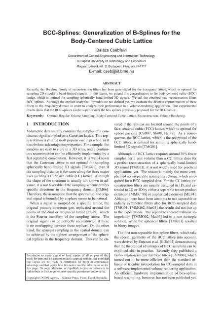
Recently, <strong>the</strong> B-spline family <strong>of</strong> reconstruction filters has been generalized <strong>for</strong> <strong>the</strong> hexagonal lattice, which is optimal <strong>for</strong><br />
sampling 2D circularly band-limited signals. In this paper, we extend this generalization to <strong>the</strong> body-centered cubic (<strong>BCC</strong>)<br />
lattice, which is optimal <strong>for</strong> sampling spherically band-limited 3D signals. We call <strong>the</strong> obtained new reconstruction filters<br />
<strong>BCC</strong>-splines. Although <strong>the</strong> explicit analytical <strong>for</strong>mulas are not defined yet, we evaluate <strong>the</strong> discrete approximation <strong>of</strong> <strong>the</strong>se<br />
filters in <strong>the</strong> frequency domain in order to analyze <strong>the</strong>ir per<strong>for</strong>mance in a volume-rendering application. Our experimental<br />
results show that <strong>the</strong> <strong>BCC</strong>-splines can be superior over <strong>the</strong> box splines previously proposed <strong>for</strong> <strong>the</strong> <strong>BCC</strong> lattice.<br />
Keywords: Optimal Regular Volume Sampling, <strong>Body</strong>-<strong>Centered</strong> Cubic Lattice, Reconstruction, Volume Rendering.<br />
1 INTRODUCTION<br />
Volumetric data usually contains <strong>the</strong> samples <strong>of</strong> a continuous<br />
signal sampled on a Cartesian lattice. This representation<br />
is still <strong>the</strong> most popular one in practice, as it<br />
has obvious advantageous properties. For example, <strong>the</strong><br />
samples are easy to store in a 3D array, and a continuous<br />
reconstruction can be efficiently implemented by a<br />
fast separable convolution. However, it is well-known<br />
that <strong>the</strong> Cartesian lattice is not optimal <strong>for</strong> sampling<br />
spherically band-limited 3D signals [TMG01], even if<br />
<strong>the</strong> sampling distance is <strong>the</strong> same along <strong>the</strong> three major<br />
axes yielding a Cartesian cubic (CC) lattice. Although<br />
<strong>the</strong> shape <strong>of</strong> <strong>the</strong> spectrum is usually not known in advance,<br />
it is not favorable if <strong>the</strong> sampling scheme prefers<br />
specific directions in <strong>the</strong> frequency domain [EM06].<br />
There<strong>for</strong>e, <strong>the</strong> assumption that <strong>the</strong> spectrum <strong>of</strong> <strong>the</strong> original<br />
signal is bounded by a sphere seems to be natural.<br />
When a signal is sampled on a specific lattice, <strong>the</strong><br />
original primary spectrum gets replicated around <strong>the</strong><br />
points <strong>of</strong> <strong>the</strong> dual or reciprocal lattice [OS89], which<br />
is <strong>the</strong> Fourier trans<strong>for</strong>m <strong>of</strong> <strong>the</strong> sampling lattice. The<br />
original signal can be perfectly reconstructed if <strong>the</strong>re<br />
is no overlapping between <strong>the</strong>se replicas. On <strong>the</strong> o<strong>the</strong>r<br />
hand, <strong>the</strong> sparsest sampling in <strong>the</strong> spatial domain can<br />
be achieved by <strong>the</strong> tightest arrangement <strong>of</strong> <strong>the</strong> spherical<br />
replicas in <strong>the</strong> frequency domain. This can be en-<br />
Permission to make digital or hard copies <strong>of</strong> all or part <strong>of</strong> this<br />
work <strong>for</strong> personal or classroom use is granted without fee provided<br />
that copies are not made or distributed <strong>for</strong> pr<strong>of</strong>it or commercial<br />
advantage and that copies bear this notice and <strong>the</strong> full citation on <strong>the</strong><br />
first page. To copy o<strong>the</strong>rwise, or republish, to post on servers or to<br />
redistribute to lists, requires prior specific permission and/or a fee.<br />
Copyright UNION Agency – Science Press, Plzen, Czech Republic.<br />
sured if <strong>the</strong> replicas are located around <strong>the</strong> points <strong>of</strong> a<br />
face-centered cubic (FCC) lattice, which is optimal <strong>for</strong><br />
sphere packing [CSB87, Slo98, Hal98]. As a consequence,<br />
<strong>the</strong> <strong>BCC</strong> lattice, which is <strong>the</strong> reciprocal <strong>of</strong> <strong>the</strong><br />
FCC lattice, is optimal <strong>for</strong> sampling spherically bandlimited<br />
3D signals [TMG01].<br />
Although <strong>the</strong> <strong>BCC</strong> lattice requires around 30% fewer<br />
samples per a unit volume than a CC lattice does <strong>for</strong><br />
a perfect reconstruction <strong>of</strong> a spherically band-limited<br />
3D signal [TMG01], it is not widely used <strong>for</strong> practical<br />
applications yet. The reason is mainly <strong>the</strong> more complicated<br />
non-separable resampling scheme, which is required<br />
<strong>for</strong> a <strong>BCC</strong>-sampled data. For <strong>the</strong> CC lattice, reconstruction<br />
filters are usually designed in 1D, and extended<br />
to 2D or 3D by ei<strong>the</strong>r a separable tensor-product<br />
extension [MMK + 98] or a spherical extension [ML94].<br />
Although <strong>the</strong>re have been attempts to use separable or<br />
radially symmetric filters also <strong>for</strong> <strong>BCC</strong>-sampled data<br />
[TMG01, TMMG02, Mat03], <strong>the</strong> results did not live up<br />
to <strong>the</strong> expectations. The separable sheared trilinear interpolation<br />
[TMMG02, Mat03] led to a non-isotropic<br />
solution, while <strong>the</strong> spherical filters [TMG01] resulted<br />
in blurry images.<br />
The first non-separable box-spline filters, which take<br />
<strong>the</strong> special geometry <strong>of</strong> <strong>the</strong> <strong>BCC</strong> lattice into account,<br />
were derived by Entezari et al. [EDM04] demonstrating<br />
that <strong>the</strong> <strong>the</strong>oretical advantages <strong>of</strong> <strong>BCC</strong> sampling can be<br />
exploited also in practice. Recently <strong>the</strong>y published a<br />
fast evaluation scheme <strong>for</strong> <strong>the</strong>se filters [EVM08], which<br />
turned out to be more efficient than <strong>the</strong> standard trilinear<br />
or tricubic interpolation <strong>for</strong> CC-sampled data in<br />
a s<strong>of</strong>tware-implemented volume-rendering application.<br />
An efficient hardware implementation <strong>of</strong> box-splinebased<br />
resampling, however, has not been published yet.
Csébfalvi recommended a prefiltered reconstruction<br />
scheme [Csé05], adapting <strong>the</strong> concept <strong>of</strong> generalized<br />
interpolation [BTU99] to <strong>the</strong> <strong>BCC</strong> lattice. According to<br />
this approach, first a non-separable discrete prefiltering<br />
is per<strong>for</strong>med as a preprocessing, and afterwards a fast<br />
separable Gaussian filtering is used <strong>for</strong> a continuous resampling<br />
on <strong>the</strong> fly. Note that <strong>the</strong> resulting impulse<br />
response is non-separable and not even radially symmetric.<br />
This method was extended also to <strong>the</strong> B-spline<br />
family <strong>of</strong> filters [CH06], and exploiting <strong>the</strong> separable<br />
postfiltering, an efficient hardware implementation was<br />
proposed.<br />
In this paper, <strong>the</strong> B-splines are generalized to <strong>the</strong><br />
<strong>BCC</strong> lattice analogously to <strong>the</strong> Hex-splines. The Hexsplines<br />
were proposed by Van de Ville et al. <strong>for</strong> <strong>the</strong><br />
hexagonal lattice [VBU04], which is optimal <strong>for</strong> sampling<br />
circularly band-limited 2D signals. The key idea<br />
is to take <strong>the</strong> indicator function <strong>of</strong> <strong>the</strong> Voronoi cell corresponding<br />
to <strong>the</strong> <strong>BCC</strong> lattice as a generating function.<br />
The successive convolutions <strong>of</strong> this generating function<br />
with itself yield <strong>the</strong> family <strong>of</strong> our <strong>BCC</strong>-splines. In <strong>the</strong><br />
following we empirically show that a <strong>BCC</strong>-spline can<br />
be superior over a box spline <strong>of</strong> <strong>the</strong> same order <strong>of</strong> approximation.<br />
2 THE B-SPLINE FAMILY OF FIL-<br />
TERS<br />
In this section we shortly review <strong>the</strong> B-spline family<br />
<strong>of</strong> filters, as we will generalize <strong>the</strong>m <strong>for</strong> <strong>the</strong> <strong>the</strong> <strong>BCC</strong><br />
lattice. The B-spline <strong>of</strong> order zero is defined as a symmetric<br />
box filter:<br />
⎧<br />
⎨1if|t| < 1<br />
β 0 2<br />
(t)= 1<br />
⎩ 2<br />
if |t| = 1 (1)<br />
2<br />
0 o<strong>the</strong>rwise.<br />
The non-symmetric nearest-neighbor interpolation kernel<br />
and β 0 (t) are almost identical, <strong>the</strong>y differ from each<br />
o<strong>the</strong>r only at <strong>the</strong> transition values. Generally, <strong>the</strong> B-<br />
spline filter <strong>of</strong> order n is derived by successively convolving<br />
β 0 (t) n times with itself. The first-order B-<br />
spline is <strong>the</strong> linear interpolation filter:<br />
{<br />
β 1 (t)=β 0 (t) ∗ β 0 (t)= 1 −|t| if |t|≤1<br />
(2)<br />
0 o<strong>the</strong>rwise.<br />
Higher-order B-splines are only approximation filters,<br />
as <strong>the</strong>y do not satisfy <strong>the</strong> interpolation constraint. For<br />
example, <strong>the</strong> cubic B-spline results in a smooth C 2<br />
continuous approximation, <strong>the</strong>re<strong>for</strong>e it is <strong>of</strong>ten used<br />
in practice to reconstruct signals that are corrupted by<br />
noise. The cubic B-spline is defined as follows:<br />
⎧<br />
⎨<br />
1<br />
β 3 2 |t|3 −|t| 2 + 2 3<br />
if |t|≤1<br />
(t)=<br />
⎩− 1 6 |t|3 + |t| 2 − 2|t| + 4 3<br />
if 1 < |t|≤2 (3)<br />
0 o<strong>the</strong>rwise.<br />
Since <strong>the</strong> Fourier trans<strong>for</strong>m <strong>of</strong> β 0 (t) is sinc(ω/2) =<br />
sin(ω/2)/(ω/2) and <strong>the</strong> consecutive convolutions in<br />
<strong>the</strong> spatial domain correspond to consecutive multiplications<br />
in <strong>the</strong> frequency domain, <strong>the</strong> Fourier trans<strong>for</strong>m<br />
<strong>of</strong> β n (t) is sinc n+1 (ω/2).<br />
Note that <strong>the</strong> frequency response <strong>of</strong> any B-spline<br />
takes a value <strong>of</strong> zero at <strong>the</strong> centers <strong>of</strong> all <strong>the</strong> aliasing<br />
spectra (if ω = j2π, where j ∈ Z \{0}), <strong>the</strong>re<strong>for</strong>e a<br />
sample frequency ripple [ML94] cannot occur. This<br />
postaliasing effect arises when <strong>the</strong> frequency response<br />
<strong>of</strong> <strong>the</strong> filter is significantly non-zero at <strong>the</strong> positions representing<br />
<strong>the</strong> “DC” component <strong>of</strong> <strong>the</strong> aliasing spectra,<br />
and appears in <strong>the</strong> reconstructed signal as an oscillation<br />
at <strong>the</strong> sample frequency.<br />
The 1D B-splines can be extended to higherdimensional<br />
Cartesian lattices by a tensor product<br />
extension. It is easy to see that such an extension <strong>of</strong> a<br />
B-spline <strong>of</strong> order n provides an approximation order<br />
<strong>of</strong> n + 1 as <strong>the</strong> multiplicity <strong>of</strong> zero at <strong>the</strong> dual lattice<br />
points (except <strong>the</strong> origin) is at least n + 1 [SF71].<br />
Figure 1: The Voronoi cell <strong>of</strong> <strong>the</strong> <strong>BCC</strong> lattice.<br />
3 GENERALIZATION FOR THE <strong>BCC</strong><br />
LATTICE<br />
The separable 3D B-spline <strong>of</strong> order zero is actually <strong>the</strong><br />
indicator function <strong>of</strong> <strong>the</strong> Voronoi cell corresponding to<br />
<strong>the</strong> Cartesian lattice. Fur<strong>the</strong>rmore, <strong>the</strong> higher-order 3D<br />
B-splines can also be obtained by <strong>the</strong> successive 3D<br />
convolutions <strong>of</strong> this indicator function. This concept<br />
can be generalized to <strong>the</strong> <strong>BCC</strong> lattice by taking <strong>the</strong> indicator<br />
function <strong>of</strong> its Voronoi cell (see Figure 1) at <strong>the</strong><br />
origin as a generating function:<br />
{ 1ifx ∈ Voronoi cell,<br />
1<br />
χ <strong>BCC</strong> (x)=<br />
m x<br />
if x ∈ boundary <strong>of</strong> <strong>the</strong> Voronoi cell,<br />
0ifx /∈ Voronoi cell,<br />
(4)<br />
where m x is <strong>the</strong> number <strong>of</strong> Voronoi cells adjacent at<br />
point x. We define <strong>the</strong> <strong>BCC</strong>-spline <strong>of</strong> order zero as<br />
β<strong>BCC</strong> 0 (x) =χ <strong>BCC</strong>(x). <strong>BCC</strong>-splines <strong>of</strong> higher orders are<br />
constructed by successive convolutions:<br />
n<br />
<strong>BCC</strong> (x)=(β <strong>BCC</strong> ∗ β <strong>BCC</strong> 0 )(x) , (5)<br />
Ω<br />
β n+1
5 EXPERIMENTAL RESULTS<br />
where Ω is a normalization term defined as <strong>the</strong> integral<br />
β<strong>BCC</strong> n (x) equals to n + 1. less annoying artifacts, and it reconstructs <strong>the</strong> high-<br />
<strong>of</strong> χ <strong>BCC</strong> (x):<br />
∫<br />
Non-separable 3D filters have been proposed <strong>for</strong> <strong>the</strong><br />
Ω = <strong>BCC</strong>(x)dx. (6) <strong>BCC</strong> and FCC lattices [EDM04, QEE + 05], and recently<br />
even <strong>for</strong> <strong>the</strong> separable CC lattice [EM06]. Due to<br />
x∈R 3 <strong>the</strong>ir non-separability, however, <strong>the</strong>se filters are ei<strong>the</strong>r<br />
spatial domain frequency domain difficult to express by a simple closed <strong>for</strong>m, or computationally<br />
T 4 /T<br />
expensive to evaluate. Never<strong>the</strong>less, <strong>the</strong>ir im-<br />
pulse response can be evaluated in a 3D lookup table in<br />
a preprocessing, and afterwards such a discrete approximation<br />
can be used <strong>for</strong> a fast resampling on <strong>the</strong> fly.<br />
Higher-order non-separable filters defined by successive<br />
convolutions <strong>of</strong> a generating function are usually<br />
evaluated in <strong>the</strong> frequency domain [QEE + 05, EM06],<br />
where <strong>the</strong> convolution is replaced by a multiplication.<br />
We apply <strong>the</strong> same approach <strong>for</strong> our <strong>BCC</strong>-splines <strong>of</strong><br />
higher orders as well.<br />
3<br />
Ш <strong>BCC</strong> ( x/T)/T<br />
Ш FCC ( )<br />
<br />
Each successive convolution <strong>of</strong> <strong>the</strong> generating function<br />
increases <strong>the</strong> support <strong>of</strong> <strong>the</strong> resulting <strong>BCC</strong>-spline<br />
Figure 2: Duality between <strong>the</strong> FCC and <strong>BCC</strong> lattices. filter, but its shape remains <strong>the</strong> same as that <strong>of</strong> <strong>the</strong><br />
4 ORDER OF APPROXIMATION<br />
Voronoi cell, which is a truncated octahedron (see Figure<br />
1). The slices <strong>of</strong> <strong>the</strong> first-order <strong>BCC</strong>-spline β<strong>BCC</strong> 1 (x)<br />
Note that β<strong>BCC</strong> 0 (x) guarantees a partition <strong>of</strong> unity by definition,<br />
thus it tiles <strong>the</strong> 3D space on a <strong>BCC</strong> pattern: are interpolating filters (β<strong>BCC</strong> 1 (x) vanishes reaching <strong>the</strong><br />
are shown in Figure 3. Note that β<strong>BCC</strong> 0 (x) and β <strong>BCC</strong> 1 (x)<br />
first neighboring lattice points), while <strong>the</strong> higher-order<br />
X <strong>BCC</strong> (x) ∗ β<strong>BCC</strong> 0 (x)=1, (7) <strong>BCC</strong>-splines are just approximating filters.<br />
where X <strong>BCC</strong> (x) is a shah function defined on <strong>the</strong> <strong>BCC</strong><br />
lattice (see Figure 2). Trans<strong>for</strong>ming Equation 7 into <strong>the</strong><br />
frequency domain (see <strong>the</strong> details in <strong>the</strong> Appendix), we<br />
obtain:<br />
1<br />
( ω<br />
)<br />
4 X FCC ·<br />
4π<br />
( ω<br />
)<br />
<strong>BCC</strong> 0 (ω)=δ .<br />
2π<br />
(8)<br />
According to Equation 8, <strong>the</strong> Fourier trans<strong>for</strong>m<br />
ˆβ<br />
<strong>BCC</strong> 0 (ω) <strong>of</strong> β <strong>BCC</strong> 0 (x) takes <strong>the</strong> value <strong>of</strong> Ω at <strong>the</strong><br />
origin and equals to zero at all <strong>the</strong> o<strong>the</strong>r FCC lattice<br />
points. There<strong>for</strong>e, based on <strong>the</strong> well-known Strang-Fix<br />
conditions [SF71], an approximation order <strong>of</strong> one<br />
is ensured by β<strong>BCC</strong> 0 (x). The order <strong>of</strong> approximation<br />
Figure 3: Slices <strong>of</strong> <strong>the</strong> first-order <strong>BCC</strong>-spline.<br />
is an asymptotic measure, which expresses how fast<br />
<strong>the</strong> approximate signal ˜f (x) converges to <strong>the</strong> original In order to empirically compare <strong>the</strong> <strong>BCC</strong>-splines to<br />
signal f (x), when <strong>the</strong> distance T between <strong>the</strong> samples <strong>the</strong> box splines <strong>of</strong> <strong>the</strong> same approximation orders, we<br />
is decreased. According to <strong>the</strong> approximation <strong>the</strong>ory, implemented a s<strong>of</strong>tware ray caster, which uses a precalculated<br />
3D lookup table <strong>of</strong> resolution 256 3 <strong>for</strong> rep-<br />
it depends only on <strong>the</strong> reconstruction filter φ(x) that is<br />
convolved with <strong>the</strong> original <strong>BCC</strong> samples <strong>of</strong> f (x): resenting <strong>the</strong> approximate filter kernels. First, we rendered<br />
<strong>the</strong> classical Marschner-Lobb test signal sampled<br />
f (x) ≈ ˜f (x)= X <strong>BCC</strong>(x/T ) · f (x)<br />
T 3 ∗ φ(x/T ). (9) at resolutions <strong>of</strong> 32×32×32×2, 64×64×64×2, and<br />
96×96×96×2. In Figure 4 <strong>the</strong> first-order <strong>BCC</strong>-spline<br />
To ensure that || ˜f (x) − f (x)|| tends to zero as T L , <strong>the</strong><br />
approximation order <strong>of</strong> <strong>the</strong> filter φ(x) should necessarily<br />
be L. When higher-order <strong>BCC</strong>-splines are constructed,<br />
each successive convolution (which is equivalent<br />
to a successive multiplication in <strong>the</strong> frequency<br />
domain) increases <strong>the</strong> multiplicity <strong>of</strong> zeros (or vanishing<br />
moments) by one, thus <strong>the</strong> approximation order <strong>of</strong><br />
is compared to <strong>the</strong> linear box spline <strong>of</strong> <strong>the</strong> same approximation<br />
order. The upper six images show <strong>the</strong> shaded<br />
isosurface <strong>of</strong> <strong>the</strong> test signal, whereas <strong>the</strong> lower six images<br />
show <strong>the</strong> angular error <strong>of</strong> <strong>the</strong> gradients calculated<br />
by central differencing on <strong>the</strong> reconstructed function.<br />
Although both filters ensure approximately <strong>the</strong> same<br />
speed <strong>of</strong> convergence, <strong>the</strong> <strong>BCC</strong>-spline produces much
frequency components significantly better, especially<br />
when <strong>the</strong> original signal is not oversampled.<br />
Figure 5 shows <strong>the</strong> comparison <strong>of</strong> <strong>the</strong> third-order<br />
<strong>BCC</strong>-spline to <strong>the</strong> cubic box spline 1 <strong>of</strong> <strong>the</strong> same<br />
approximation order. In this case, both filters provide<br />
approximately <strong>the</strong> same image quality and convergence<br />
to <strong>the</strong> original signal. However, <strong>the</strong> <strong>BCC</strong>-spline leads<br />
to slightly stronger oversmoothing <strong>for</strong> <strong>the</strong> lowerresolution<br />
representation. For rendering data sets <strong>of</strong><br />
high signal-to-noise ratio this is clearly a drawback, as<br />
<strong>the</strong> high-frequency details might be removed. On <strong>the</strong><br />
o<strong>the</strong>r hand, practical data sets are usually corrupted by<br />
noise, which can be suppressed by a filter <strong>of</strong> stronger<br />
oversmoothing. In order to test <strong>the</strong> <strong>BCC</strong>-splines on a<br />
real world data set as well, we downsampled an MRI<br />
scan <strong>of</strong> a human brain consisting <strong>of</strong> 256 × 256 × 166<br />
CC samples onto a lower resolution <strong>BCC</strong> lattice<br />
yielding 128 × 128 × 83 × 2 <strong>BCC</strong> samples. Entezari et<br />
al. used a similar downsampling [EMBM06] to obtain<br />
a <strong>BCC</strong> representation <strong>of</strong> an originally CC-sampled<br />
data set. However, we exploited that in <strong>the</strong> frequency<br />
domain a perfect low-pass filtering can be per<strong>for</strong>med<br />
be<strong>for</strong>e <strong>the</strong> subsampling. There<strong>for</strong>e we multiplied <strong>the</strong><br />
discrete Fourier trans<strong>for</strong>m <strong>of</strong> <strong>the</strong> original CC-sampled<br />
data by <strong>the</strong> indicator function <strong>of</strong> <strong>the</strong> FCC Voronoi<br />
cell, that is, <strong>the</strong> frequency response <strong>of</strong> <strong>the</strong> ideal<br />
low-pass filter <strong>for</strong> <strong>BCC</strong> downsampling. Afterwards<br />
we trans<strong>for</strong>med <strong>the</strong> data back into <strong>the</strong> spatial domain<br />
and took <strong>the</strong> samples <strong>of</strong> <strong>the</strong> <strong>BCC</strong> sublattice. Figure 6<br />
shows <strong>the</strong> reconstruction <strong>of</strong> <strong>the</strong> human brain from<br />
<strong>the</strong> 128 × 128 × 83 × 2 <strong>BCC</strong> samples. The images<br />
demonstrate that artifacts caused by <strong>the</strong> noise and<br />
postaliasing are better reduced by <strong>the</strong> <strong>BCC</strong>-splines than<br />
by <strong>the</strong> box splines <strong>of</strong> <strong>the</strong> same approximation orders.<br />
Concerning <strong>the</strong> computational cost, <strong>the</strong> <strong>BCC</strong>-splines<br />
<strong>of</strong> order one and three require 8 and 64 neighboring<br />
voxels to access respectively. It is interesting to note<br />
that <strong>the</strong> equivalent B-splines <strong>for</strong> <strong>the</strong> Cartesian lattice require<br />
exactly <strong>the</strong> same number <strong>of</strong> voxels to read. Never<strong>the</strong>less,<br />
using a 3D lookup table to approximate <strong>the</strong><br />
filter kernels, <strong>the</strong> <strong>BCC</strong>-splines are about twice as expensive<br />
to evaluate than <strong>the</strong> box splines <strong>of</strong> <strong>the</strong> same<br />
approximation orders, since <strong>the</strong> linear and cubic box<br />
splines need just 4 and 32 neighboring voxels to take<br />
into account respectively. Thus, <strong>the</strong> price <strong>of</strong> <strong>the</strong> quality<br />
improvement is <strong>the</strong> additional computational cost.<br />
6 CONCLUSION AND FUTURE<br />
WORK<br />
In this paper a new family <strong>of</strong> filters has been proposed<br />
<strong>for</strong> <strong>the</strong> <strong>BCC</strong> lattice, which can be interpreted as a non-<br />
1 In [EDM04] <strong>the</strong> convolution <strong>of</strong> <strong>the</strong> linear box spline with itself is<br />
referred to as a “cubic box spline” as it provides <strong>the</strong> same approximation<br />
power as <strong>the</strong> tricubic B-spline <strong>for</strong> <strong>the</strong> CC lattice. Throughout<br />
this paper we also use <strong>the</strong> term “cubic box spline”, although this filter<br />
is quintic in fact [EVM08], as it consists <strong>of</strong> quintic polynomials.<br />
separable generalization <strong>of</strong> <strong>the</strong> separable tensor-product<br />
extension <strong>of</strong> B-splines. It has been empirically demonstrated<br />
that, <strong>for</strong> an additional computational ef<strong>for</strong>t, our<br />
<strong>BCC</strong>-splines can provide higher image quality than <strong>the</strong><br />
box splines <strong>of</strong> <strong>the</strong> same approximation orders. For our<br />
experiments we approximately evaluated <strong>the</strong> filter kernels<br />
in <strong>the</strong> frequency domain.<br />
The derivation <strong>of</strong> <strong>the</strong> explicit analytical <strong>for</strong>mulas,<br />
however, is <strong>the</strong> subject <strong>of</strong> our future work. Recently<br />
it has been shown that a cubic box spline can be efficiently<br />
evaluated by factorizing <strong>the</strong> filter into a finite<br />
difference operator and its Green’s function corresponding<br />
to <strong>the</strong> given filter kernel [EVM08]. We plan<br />
to follow a similar strategy <strong>for</strong> <strong>the</strong> efficient analytical<br />
evaluation <strong>of</strong> our <strong>BCC</strong>-splines. This would be favorable<br />
<strong>for</strong> a fast hardware implementation as well, since<br />
<strong>the</strong> 3D lookup table representing <strong>the</strong> approximate filter<br />
kernel would not take <strong>the</strong> texture memory from larger<br />
data sets. Fur<strong>the</strong>rmore, we would like to derive <strong>the</strong> frequency<br />
responses <strong>of</strong> <strong>the</strong>se filters in order to quantitatively<br />
measure <strong>the</strong>ir postaliasing and oversmoothing effect.<br />
An additional possibility <strong>for</strong> improving <strong>the</strong> reconstruction<br />
<strong>of</strong> <strong>BCC</strong>-sampled data is to use a discrete prefiltering<br />
be<strong>for</strong>e <strong>the</strong> continuous filtering. For example,<br />
<strong>the</strong> approximation power <strong>of</strong> higher-order <strong>BCC</strong>-splines<br />
could be better exploited by applying prefitered interpolation<br />
or quasi-interpolation schemes.<br />
ACKNOWLEDGEMENTS<br />
This work was supported by <strong>the</strong> János Bolyai Research<br />
Scholarship <strong>of</strong> <strong>the</strong> Hungarian Academy <strong>of</strong> Sciences,<br />
OTKA (F68945), <strong>the</strong> Hungarian National Office <strong>for</strong> Research<br />
and Technology, and Hewlett-Packard. The author<br />
<strong>of</strong> this paper is a grantee <strong>of</strong> <strong>the</strong> János Bolyai Scholarship.<br />
Special thanks to Alireza Entezari <strong>for</strong> providing<br />
<strong>the</strong> source code <strong>of</strong> his linear and cubic box-spline reconstruction<br />
routines.<br />
APPENDIX<br />
The shah function <strong>for</strong> <strong>the</strong> <strong>BCC</strong> lattice is defined as two<br />
overlapping Cartesian shah functions:<br />
X <strong>BCC</strong> (x)=<br />
∑<br />
i, j,k∈Z<br />
δ(x − [i, j,k] T )+ (10)<br />
( [<br />
∑ δ x − i + 1<br />
i, j,k∈Z<br />
2 , j + 1 2 ,k + 1 ] ) T<br />
.<br />
2<br />
Analogously, <strong>the</strong> shah function <strong>for</strong> <strong>the</strong> FCC lattice is<br />
constructed as four overlapping Cartesian shah functions:<br />
X FCC (x)=<br />
∑<br />
i, j,k∈Z<br />
δ(x − [i, j,k] T )+ (11)<br />
( [<br />
∑ δ x − i, j + 1<br />
i, j,k∈Z<br />
2 ,k + 1 ] ) T<br />
+<br />
2
( [<br />
∑ δ x − i + 1<br />
i, j,k∈Z<br />
2 , j,k + 1 ] ) T<br />
+<br />
2<br />
(<br />
∑ δ x −<br />
[i + 1<br />
i, j,k∈Z<br />
2 , j + 1 ] ) T<br />
2 ,k .<br />
The Fourier trans<strong>for</strong>m <strong>of</strong> X <strong>BCC</strong> is derived as follows:<br />
X <strong>BCC</strong> (x) ⇐⇒<br />
∑<br />
i, j,k∈Z<br />
δ<br />
( ω<br />
2π − [i, j,k]T ) + (12)<br />
( ω<br />
∑<br />
) δ<br />
i, j,k∈Z<br />
2π − [i, j,k]T · e J [ 1 2 , 2 1 , 1 2]ω<br />
( ω<br />
= ∑<br />
)( δ<br />
i, j,k∈Z<br />
2π − [i, j,k]T 1 +(−1)<br />
(i+ j+k))<br />
In Equation 12 only those terms are non-zero, where i+<br />
j + k is even. This is possible if all <strong>the</strong>se three integers<br />
are even, or two <strong>of</strong> <strong>the</strong>m are odd and one is even. Thus<br />
we can separate <strong>the</strong> sum into four terms:<br />
X <strong>BCC</strong> (x) ⇐⇒<br />
∑<br />
l,m,n∈Z<br />
δ<br />
( ω<br />
2π − [2l,2m,2n]T ) · 2+<br />
( ω<br />
∑<br />
) δ<br />
l,m,n∈Z<br />
2π − [2l,2m + 1,2n + 1]T · 2+<br />
( ω<br />
∑<br />
) δ<br />
l,m,n∈Z<br />
2π − [2l + 1,2m,2n + 1]T · 2+<br />
( ω<br />
∑<br />
) δ<br />
l,m,n∈Z<br />
2π − [2l + 1,2m + 1,2n]T · 2<br />
Exploiting that δ(Aω)=δ(ω)/det(A), we obtain:<br />
X <strong>BCC</strong> (x) ⇐⇒<br />
∑<br />
l,m,n∈Z<br />
(13)<br />
( ω ) δ<br />
4π − [l,m,n]T · 1<br />
4 + (14)<br />
(<br />
ω<br />
∑ δ<br />
[l,m<br />
l,m,n∈Z<br />
4π − + 1 2 ,n + 1 ] ) T<br />
2<br />
(<br />
ω<br />
∑ δ<br />
[l<br />
l,m,n∈Z<br />
4π − + 1 2 ,m,n + 1 ] ) T<br />
2<br />
( [<br />
ω<br />
∑ δ<br />
l,m,n∈Z<br />
4π − l + 1 2 ,m + 1 ] ) T<br />
2 ,n · 1<br />
4<br />
REFERENCES<br />
[BTU99]<br />
[CH06]<br />
= 1 4 X FCC<br />
( ω<br />
4π<br />
)<br />
.<br />
· 1<br />
4 +<br />
· 1<br />
4 +<br />
T. Blu, P. Thévenaz, and M. Unser. Generalized interpolation:<br />
Higher quality at no additional cost. In Proceedings<br />
<strong>of</strong> IEEE International Conference on Image<br />
Processing, pages 667–671, 1999.<br />
B. Csébfalvi and M. Hadwiger. Prefiltered B-spline reconstruction<br />
<strong>for</strong> hardware-accelerated rendering <strong>of</strong> optimally<br />
sampled volumetric data. In Proceedings <strong>of</strong><br />
Vision, Modeling, and Visualization, pages 325–332,<br />
2006.<br />
[CSB87] J. H. Conway, N. J. A. Sloane, and E. Bannai. Spherepackings,<br />
lattices, and groups. Springer-Verlag New<br />
York, Inc., 1987.<br />
[Csé05] B. Csébfalvi. Prefiltered Gaussian reconstruction <strong>for</strong><br />
high-quality rendering <strong>of</strong> volumetric data sampled on<br />
a body-centered cubic grid. In Proceedings <strong>of</strong> IEEE<br />
Visualization, pages 311–318, 2005.<br />
[EDM04] A. Entezari, R. Dyer, and T. Möller. Linear and cubic<br />
box splines <strong>for</strong> <strong>the</strong> body centered cubic lattice. In Proceedings<br />
<strong>of</strong> IEEE Visualization, pages 11–18, 2004.<br />
[EM06] A. Entezari and T. Möller. Extensions <strong>of</strong> <strong>the</strong> Zwart-<br />
Powell box spline <strong>for</strong> volumetric data reconstruction on<br />
<strong>the</strong> Cartesian lattice. IEEE Transactions on Visualization<br />
and Computer Graphics (Proceedings <strong>of</strong> IEEE Visualization),<br />
12(5):1337–1344, 2006.<br />
[EMBM06] A. Entezari, T. Meng, S. Bergner, and T. Möller. A<br />
granular three dimensional multiresolution trans<strong>for</strong>m.<br />
In Proceedings <strong>of</strong> Joint EUROGRAPHICS-IEEE VGTC<br />
Symposium on Visualization, pages 267–274, 2006.<br />
[EVM08] A. Entezari, D. Van De Ville, and T. Möller. Practical<br />
box splines <strong>for</strong> reconstruction on <strong>the</strong> body centered<br />
cubic lattice. to appear in IEEE Transactions on Visualization<br />
and Computer Graphics, 2008.<br />
[Hal98] T. C. Hales. Cannonballs and honeycombs. AMS,<br />
47(4):440–449, 1998.<br />
[Mat03] O. Mattausch. Practical reconstruction schemes and<br />
hardware-accelerated direct volume rendering on bodycentered<br />
cubic grids. Master’s Thesis, Vienna University<br />
<strong>of</strong> Technology, 2003.<br />
[ML94] S. Marschner and R. Lobb. An evaluation <strong>of</strong> reconstruction<br />
filters <strong>for</strong> volume rendering. In Proceedings<br />
<strong>of</strong> IEEE Visualization, pages 100–107, 1994.<br />
[MMK + 98] T. Möller, K. Mueller, Y. Kurzion, R. Machiraju, and<br />
R. Yagel. Design <strong>of</strong> accurate and smooth filters <strong>for</strong><br />
function and derivative reconstruction. In Proceedings<br />
<strong>of</strong> IEEE Symposium on Volume Visualization, pages<br />
143–151, 1998.<br />
[OS89] A. V. Oppenheim and R. W. Schafer. Discrete-Time Signal<br />
Processing. Prentice Hall Inc., Englewood Cliffs,<br />
2nd edition, 1989.<br />
[QEE + 05] W. Quiao, D. S. Ebert, A. Entezari, M. Korkusinski, and<br />
G. Klimeck. VolQD: Direct volume rendering <strong>of</strong> multimillion<br />
atom quantum dot simulations. In Proceedings<br />
<strong>of</strong> IEEE Visualization, pages 319–326, 2005.<br />
[SF71] G. Strang and G. Fix. A Fourier analysis <strong>of</strong> <strong>the</strong> finite<br />
element variational method. In Constructive Aspects <strong>of</strong><br />
Functional Analysis, pages 796–830, 1971.<br />
[Slo98] N. J. A. Sloane. The sphere packing problem. In Proceedings<br />
<strong>of</strong> International Congress <strong>of</strong> Ma<strong>the</strong>maticians,<br />
pages 387–396, 1998.<br />
[TMG01] T. Theußl, T. Möller, and M. E. Gröller. Optimal regular<br />
volume sampling. In Proceedings <strong>of</strong> IEEE Visualization,<br />
pages 91–98, 2001.<br />
[TMMG02] T. Theußl, O. Mattausch, T. Möller, and M. E. Gröller.<br />
Reconstruction schemes <strong>for</strong> high quality raycasting <strong>of</strong><br />
<strong>the</strong> body-centered cubic grid. TR-186-2-02-11, Institute<br />
<strong>of</strong> Computer Graphics and Algorithms, Vienna University<br />
<strong>of</strong> Technology, 2002.<br />
[VBU04] D. Van De Ville, T. Blu, and M. Unser. Hex-splines: A<br />
novel spline family <strong>for</strong> hexagonal lattices. IEEE Transactions<br />
on Image Processing, 13(6):758–772, 2004.
32 × 32 × 32 × 2 voxels. 64 × 64 × 64 × 2 voxels. 96 × 96 × 96 × 2 voxels.<br />
Isosurface reconstruction using <strong>the</strong> first-order <strong>BCC</strong>-spline.<br />
Isosurface reconstruction using <strong>the</strong> linear box spline.<br />
Angular error <strong>of</strong> <strong>the</strong> gradients calculated with <strong>the</strong> first-order <strong>BCC</strong>-spline.<br />
Angular error <strong>of</strong> <strong>the</strong> gradients calculated with <strong>the</strong> linear box spline.<br />
Figure 4: Reconstruction <strong>of</strong> <strong>the</strong> Marschner-Lobb signal using <strong>the</strong> first-order <strong>BCC</strong>-spline and <strong>the</strong> linear box spline<br />
<strong>of</strong> <strong>the</strong> same order <strong>of</strong> approximation. In <strong>the</strong> error images <strong>the</strong> angular error <strong>of</strong> zero degree is mapped to black,<br />
whereas <strong>the</strong> angular error <strong>of</strong> 30 degrees is mapped to white.
32 × 32 × 32 × 2 voxels. 64 × 64 × 64 × 2 voxels. 96 × 96 × 96 × 2 voxels.<br />
Isosurface reconstruction using <strong>the</strong> third-order <strong>BCC</strong>-spline.<br />
Isosurface reconstruction using <strong>the</strong> cubic box spline.<br />
Angular error <strong>of</strong> <strong>the</strong> gradients calculated with <strong>the</strong> third-order <strong>BCC</strong>-spline.<br />
Angular error <strong>of</strong> <strong>the</strong> gradients calculated with <strong>the</strong> cubic box spline.<br />
Figure 5: Reconstruction <strong>of</strong> <strong>the</strong> Marschner-Lobb signal using <strong>the</strong> third-order <strong>BCC</strong>-spline and <strong>the</strong> cubic box spline<br />
<strong>of</strong> <strong>the</strong> same order <strong>of</strong> approximation. In <strong>the</strong> error images <strong>the</strong> angular error <strong>of</strong> zero degree is mapped to black,<br />
whereas <strong>the</strong> angular error <strong>of</strong> 30 degrees is mapped to white.
Linear box spline.<br />
First-order <strong>BCC</strong>-spline.<br />
Cubic box spline.<br />
Third-order <strong>BCC</strong>-spline.<br />
Figure 6: Reconstruction <strong>of</strong> a human brain from 128 × 128 × 83 × 2 <strong>BCC</strong> samples <strong>of</strong> an MRI scan.