BCC-Splines: Generalization of B-Splines for the Body-Centered ...

Csébfalvi recommended a prefiltered reconstruction
scheme [Csé05], adapting the concept of generalized
interpolation [BTU99] to the BCC lattice. According to
this approach, first a non-separable discrete prefiltering
is performed as a preprocessing, and afterwards a fast
separable Gaussian filtering is used for a continuous resampling
on the fly. Note that the resulting impulse
response is non-separable and not even radially symmetric.
This method was extended also to the B-spline
family of filters [CH06], and exploiting the separable
postfiltering, an efficient hardware implementation was
proposed.
In this paper, the B-splines are generalized to the
BCC lattice analogously to the Hex-splines. The Hexsplines
were proposed by Van de Ville et al. for the
hexagonal lattice [VBU04], which is optimal for sampling
circularly band-limited 2D signals. The key idea
is to take the indicator function of the Voronoi cell corresponding
to the BCC lattice as a generating function.
The successive convolutions of this generating function
with itself yield the family of our BCC-splines. In the
following we empirically show that a BCC-spline can
be superior over a box spline of the same order of approximation.
2 THE B-SPLINE FAMILY OF FIL-
TERS
In this section we shortly review the B-spline family
of filters, as we will generalize them for the the BCC
lattice. The B-spline of order zero is defined as a symmetric
box filter:
⎧
⎨1if|t| < 1
β 0 2
(t)= 1
⎩ 2
if |t| = 1 (1)
2
0 otherwise.
The non-symmetric nearest-neighbor interpolation kernel
and β 0 (t) are almost identical, they differ from each
other only at the transition values. Generally, the B-
spline filter of order n is derived by successively convolving
β 0 (t) n times with itself. The first-order B-
spline is the linear interpolation filter:
{
β 1 (t)=β 0 (t) ∗ β 0 (t)= 1 −|t| if |t|≤1
(2)
0 otherwise.
Higher-order B-splines are only approximation filters,
as they do not satisfy the interpolation constraint. For
example, the cubic B-spline results in a smooth C 2
continuous approximation, therefore it is often used
in practice to reconstruct signals that are corrupted by
noise. The cubic B-spline is defined as follows:
⎧
⎨
1
β 3 2 |t|3 −|t| 2 + 2 3
if |t|≤1
(t)=
⎩− 1 6 |t|3 + |t| 2 − 2|t| + 4 3
if 1 < |t|≤2 (3)
0 otherwise.
Since the Fourier transform of β 0 (t) is sinc(ω/2) =
sin(ω/2)/(ω/2) and the consecutive convolutions in
the spatial domain correspond to consecutive multiplications
in the frequency domain, the Fourier transform
of β n (t) is sinc n+1 (ω/2).
Note that the frequency response of any B-spline
takes a value of zero at the centers of all the aliasing
spectra (if ω = j2π, where j ∈ Z \{0}), therefore a
sample frequency ripple [ML94] cannot occur. This
postaliasing effect arises when the frequency response
of the filter is significantly non-zero at the positions representing
the “DC” component of the aliasing spectra,
and appears in the reconstructed signal as an oscillation
at the sample frequency.
The 1D B-splines can be extended to higherdimensional
Cartesian lattices by a tensor product
extension. It is easy to see that such an extension of a
B-spline of order n provides an approximation order
of n + 1 as the multiplicity of zero at the dual lattice
points (except the origin) is at least n + 1 [SF71].
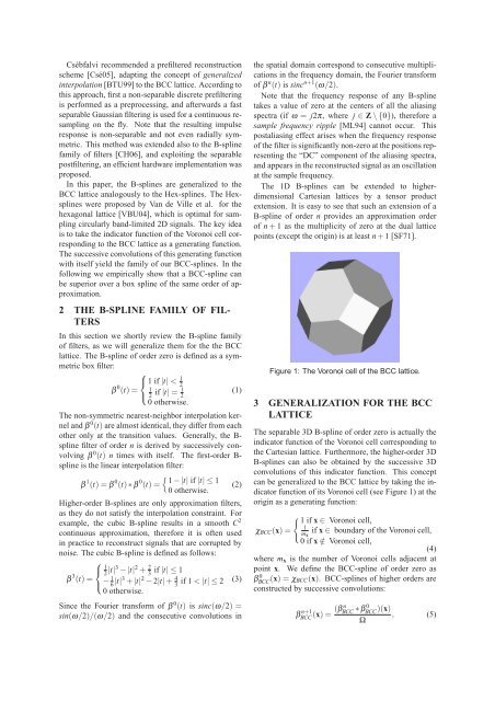
Figure 1: The Voronoi cell of the BCC lattice.
3 GENERALIZATION FOR THE BCC
LATTICE
The separable 3D B-spline of order zero is actually the
indicator function of the Voronoi cell corresponding to
the Cartesian lattice. Furthermore, the higher-order 3D
B-splines can also be obtained by the successive 3D
convolutions of this indicator function. This concept
can be generalized to the BCC lattice by taking the indicator
function of its Voronoi cell (see Figure 1) at the
origin as a generating function:
{ 1ifx ∈ Voronoi cell,
1
χ BCC (x)=
m x
if x ∈ boundary of the Voronoi cell,
0ifx /∈ Voronoi cell,
(4)
where m x is the number of Voronoi cells adjacent at
point x. We define the BCC-spline of order zero as
βBCC 0 (x) =χ BCC(x). BCC-splines of higher orders are
constructed by successive convolutions:
n
BCC (x)=(β BCC ∗ β BCC 0 )(x) , (5)
Ω
β n+1