BCC-Splines: Generalization of B-Splines for the Body-Centered ...
BCC-Splines: Generalization of B-Splines for the Body-Centered ...
BCC-Splines: Generalization of B-Splines for the Body-Centered ...

Create successful ePaper yourself
Turn your PDF publications into a flip-book with our unique Google optimized e-Paper software.
5 EXPERIMENTAL RESULTS<br />
where Ω is a normalization term defined as <strong>the</strong> integral<br />
β<strong>BCC</strong> n (x) equals to n + 1. less annoying artifacts, and it reconstructs <strong>the</strong> high-<br />
<strong>of</strong> χ <strong>BCC</strong> (x):<br />
∫<br />
Non-separable 3D filters have been proposed <strong>for</strong> <strong>the</strong><br />
Ω = <strong>BCC</strong>(x)dx. (6) <strong>BCC</strong> and FCC lattices [EDM04, QEE + 05], and recently<br />
even <strong>for</strong> <strong>the</strong> separable CC lattice [EM06]. Due to<br />
x∈R 3 <strong>the</strong>ir non-separability, however, <strong>the</strong>se filters are ei<strong>the</strong>r<br />
spatial domain frequency domain difficult to express by a simple closed <strong>for</strong>m, or computationally<br />
T 4 /T<br />
expensive to evaluate. Never<strong>the</strong>less, <strong>the</strong>ir im-<br />
pulse response can be evaluated in a 3D lookup table in<br />
a preprocessing, and afterwards such a discrete approximation<br />
can be used <strong>for</strong> a fast resampling on <strong>the</strong> fly.<br />
Higher-order non-separable filters defined by successive<br />
convolutions <strong>of</strong> a generating function are usually<br />
evaluated in <strong>the</strong> frequency domain [QEE + 05, EM06],<br />
where <strong>the</strong> convolution is replaced by a multiplication.<br />
We apply <strong>the</strong> same approach <strong>for</strong> our <strong>BCC</strong>-splines <strong>of</strong><br />
higher orders as well.<br />
3<br />
Ш <strong>BCC</strong> ( x/T)/T<br />
Ш FCC ( )<br />
<br />
Each successive convolution <strong>of</strong> <strong>the</strong> generating function<br />
increases <strong>the</strong> support <strong>of</strong> <strong>the</strong> resulting <strong>BCC</strong>-spline<br />
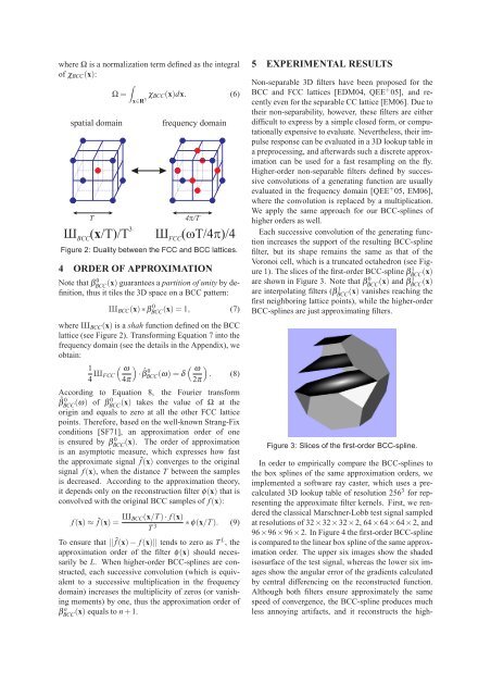
Figure 2: Duality between <strong>the</strong> FCC and <strong>BCC</strong> lattices. filter, but its shape remains <strong>the</strong> same as that <strong>of</strong> <strong>the</strong><br />
4 ORDER OF APPROXIMATION<br />
Voronoi cell, which is a truncated octahedron (see Figure<br />
1). The slices <strong>of</strong> <strong>the</strong> first-order <strong>BCC</strong>-spline β<strong>BCC</strong> 1 (x)<br />
Note that β<strong>BCC</strong> 0 (x) guarantees a partition <strong>of</strong> unity by definition,<br />
thus it tiles <strong>the</strong> 3D space on a <strong>BCC</strong> pattern: are interpolating filters (β<strong>BCC</strong> 1 (x) vanishes reaching <strong>the</strong><br />
are shown in Figure 3. Note that β<strong>BCC</strong> 0 (x) and β <strong>BCC</strong> 1 (x)<br />
first neighboring lattice points), while <strong>the</strong> higher-order<br />
X <strong>BCC</strong> (x) ∗ β<strong>BCC</strong> 0 (x)=1, (7) <strong>BCC</strong>-splines are just approximating filters.<br />
where X <strong>BCC</strong> (x) is a shah function defined on <strong>the</strong> <strong>BCC</strong><br />
lattice (see Figure 2). Trans<strong>for</strong>ming Equation 7 into <strong>the</strong><br />
frequency domain (see <strong>the</strong> details in <strong>the</strong> Appendix), we<br />
obtain:<br />
1<br />
( ω<br />
)<br />
4 X FCC ·<br />
4π<br />
( ω<br />
)<br />
<strong>BCC</strong> 0 (ω)=δ .<br />
2π<br />
(8)<br />
According to Equation 8, <strong>the</strong> Fourier trans<strong>for</strong>m<br />
ˆβ<br />
<strong>BCC</strong> 0 (ω) <strong>of</strong> β <strong>BCC</strong> 0 (x) takes <strong>the</strong> value <strong>of</strong> Ω at <strong>the</strong><br />
origin and equals to zero at all <strong>the</strong> o<strong>the</strong>r FCC lattice<br />
points. There<strong>for</strong>e, based on <strong>the</strong> well-known Strang-Fix<br />
conditions [SF71], an approximation order <strong>of</strong> one<br />
is ensured by β<strong>BCC</strong> 0 (x). The order <strong>of</strong> approximation<br />
Figure 3: Slices <strong>of</strong> <strong>the</strong> first-order <strong>BCC</strong>-spline.<br />
is an asymptotic measure, which expresses how fast<br />
<strong>the</strong> approximate signal ˜f (x) converges to <strong>the</strong> original In order to empirically compare <strong>the</strong> <strong>BCC</strong>-splines to<br />
signal f (x), when <strong>the</strong> distance T between <strong>the</strong> samples <strong>the</strong> box splines <strong>of</strong> <strong>the</strong> same approximation orders, we<br />
is decreased. According to <strong>the</strong> approximation <strong>the</strong>ory, implemented a s<strong>of</strong>tware ray caster, which uses a precalculated<br />
3D lookup table <strong>of</strong> resolution 256 3 <strong>for</strong> rep-<br />
it depends only on <strong>the</strong> reconstruction filter φ(x) that is<br />
convolved with <strong>the</strong> original <strong>BCC</strong> samples <strong>of</strong> f (x): resenting <strong>the</strong> approximate filter kernels. First, we rendered<br />
<strong>the</strong> classical Marschner-Lobb test signal sampled<br />
f (x) ≈ ˜f (x)= X <strong>BCC</strong>(x/T ) · f (x)<br />
T 3 ∗ φ(x/T ). (9) at resolutions <strong>of</strong> 32×32×32×2, 64×64×64×2, and<br />
96×96×96×2. In Figure 4 <strong>the</strong> first-order <strong>BCC</strong>-spline<br />
To ensure that || ˜f (x) − f (x)|| tends to zero as T L , <strong>the</strong><br />
approximation order <strong>of</strong> <strong>the</strong> filter φ(x) should necessarily<br />
be L. When higher-order <strong>BCC</strong>-splines are constructed,<br />
each successive convolution (which is equivalent<br />
to a successive multiplication in <strong>the</strong> frequency<br />
domain) increases <strong>the</strong> multiplicity <strong>of</strong> zeros (or vanishing<br />
moments) by one, thus <strong>the</strong> approximation order <strong>of</strong><br />
is compared to <strong>the</strong> linear box spline <strong>of</strong> <strong>the</strong> same approximation<br />
order. The upper six images show <strong>the</strong> shaded<br />
isosurface <strong>of</strong> <strong>the</strong> test signal, whereas <strong>the</strong> lower six images<br />
show <strong>the</strong> angular error <strong>of</strong> <strong>the</strong> gradients calculated<br />
by central differencing on <strong>the</strong> reconstructed function.<br />
Although both filters ensure approximately <strong>the</strong> same<br />
speed <strong>of</strong> convergence, <strong>the</strong> <strong>BCC</strong>-spline produces much