Week 6: Binomial and Poisson Models

Week 6: Binomial and Poisson Models
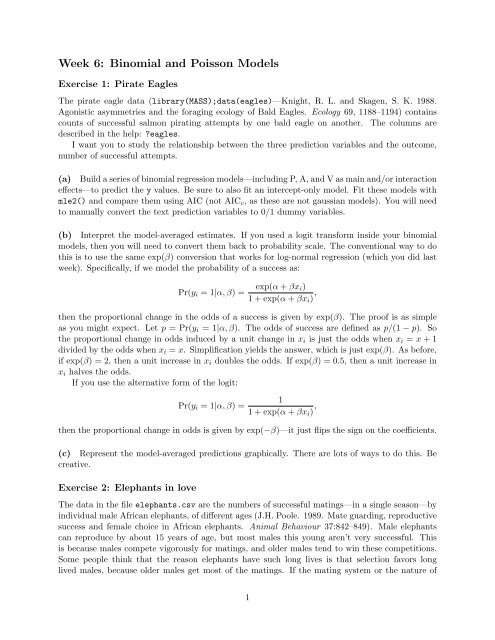
Exercise 1: Pirate Eagles
The pirate eagle data (library(MASS);data(eagles)—Knight, R. L. and Skagen, S. K. 1988.
Agonistic asymmetries and the foraging ecology of Bald Eagles. Ecology 69, 1188–1194) contains
counts of successful salmon pirating attempts by one bald eagle on another. The columns are
described in the help: ?eagles.
I want you to study the relationship between the three prediction variables and the outcome,
number of successful attempts.
(a) Build a series of binomial regression models—including P, A, and V as main and/or interaction
effects—to predict the y values. Be sure to also fit an intercept-only model. Fit these models with
mle2() and compare them using AIC (not AIC c , as these are not gaussian models). You will need
to manually convert the text prediction variables to 0/1 dummy variables.
(b) Interpret the model-averaged estimates. If you used a logit transform inside your binomial
models, then you will need to convert them back to probability scale. The conventional way to do
this is to use the same exp(β) conversion that works for log-normal regression (which you did last
week). Specifically, if we model the probability of a success as:
Pr(y i = 1|α, β) = exp(α + βx i)
1 + exp(α + βx i ) ,
then the proportional change in the odds of a success is given by exp(β). The proof is as simple
as you might expect. Let p = Pr(y i = 1|α, β). The odds of success are defined as p/(1 − p). So
the proportional change in odds induced by a unit change in x i is just the odds when x i = x + 1
divided by the odds when x i = x. Simplification yields the answer, which is just exp(β). As before,
if exp(β) = 2, then a unit increase in x i doubles the odds. If exp(β) = 0.5, then a unit increase in
x i halves the odds.
If you use the alternative form of the logit:
Pr(y i = 1|α, β) =
1
1 + exp(α + βx i ) ,
then the proportional change in odds is given by exp(−β)—it just flips the sign on the coefficients.
(c) Represent the model-averaged predictions graphically. There are lots of ways to do this. Be
creative.
Exercise 2: Elephants in love
The data in the file elephants.csv are the numbers of successful matings—in a single season—by
individual male African elephants, of different ages (J.H. Poole. 1989. Mate guarding, reproductive
success and female choice in African elephants. Animal Behaviour 37:842–849). Male elephants
can reproduce by about 15 years of age, but most males this young aren’t very successful. This
is because males compete vigorously for matings, and older males tend to win these competitions.
Some people think that the reason elephants have such long lives is that selection favors long
lived males, because older males get most of the matings. If the mating system or the nature of
1

competition were different, selection might not favor males’ living so long. (I suppose one must
ignore the female half of the species, which lives even longer than the male half, to take this theory
seriously.)
I want you to use a Poisson regression to study the relationship between age and mating success.
(a)
Plot number of matings (vertical axis) against age (horizontal axis).
(b) Fit a Poisson model—matings ∼ age—using mle2(). Compare this model to the interceptonly
model. Interpret the results, including the confidence intervals.
(c)
Plot the data again, and now overlay the predicted trend, using your estimated parameters.
Exercise 3: Las salamandras del norte
The data in salamanders.csv are abundances of salamanders (Plethodon elongatus) from 47 plots
in northern California (H.H. Welsh and A.J. Lind, 1995. Journal of Herpetology 29:198–210). You
also are given the percent forest cover and forest age for each sampled site.
(a)
Plot the abundance against percent forest cover. Is the effect of cover approximately linear?
(b) Model abundance as a linear function of percent cover, and compare this model to an alternative
simpler model. Use a Poisson distribution for abundance in each case. Plotting your fit over
the data, are you satisfied with this model or not?
(c) Try adding another model to your comparison set: λ = α exp(βx i ). Compare this model to
the other models you have fit, and also plot it over the data.
(d) Finally, can you think of a biological reason that salamanders might have been under-sampled
in the more open sites? That is, imagine salamanders are actually more abundant in the open sites
than the data suggest. What might explain the mis-match between the data collected and the
reality?
2