NMR Data Acquisition The process of data acquisition results in an ...

NMR Data Acquisition
The process of data acquisition results in an FID signal residing in the computer of the
NMR instrument. In order to properly set up the acquisition parameters, it is helpful to
understand a little about how this is accomplished. The sequence of events involved in the
acquisition of the raw data for a simple 1D 1 H spectrum on a 200 MHz instrument is as follows
(Fig. 6):
1. Wait a period of time called the Relaxation Delay for spins to reach thermal
equilibrium
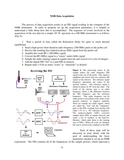
2. Send a high-power short-duration radio frequency (200 MHz) pulse to the probe coil
3. Receive the resulting free induction decay (FID) signal from the probe coil
4. Amplify this weak RF (~200 MHz) signal
5. Convert the RF (MHz) signal to a “stereo” audio (kHz) signal
6. Sample the audio (analog) signal at regular intervals and convert it to a list of integers
7. Add the digital FID “list” to a sum FID in memory
8. Repeat steps 1-8 for as many “scans” or “transients” as desired
20
Figure 6. The precessing nuclei in the
sample induce the radio frequency FID
signal in the coil of the probe. This signal is
amplified and mixed with two reference RF
signals at the detector. The reference signal
frequency determines the center of the
spectral window. One reference signal is
shifted in phase by 90 o from the other. The
result of the mixing step is an audio
frequency which is the difference between
the FID frequency and the reference
frequency. This audio frequency can be
either positive (downfield of the center of the
spectral window) or negative (upfield).
There are actually two audio signals, which
are called the "real" and the "imaginary"
parts of the FID, resulting from mixing with
either a 0 o or a 90 o reference frequency.
The analog-to-digital (ADC) converter
samples these FIDs at regular intervals and
sends a list of numbers to the Sum-To-
Memory, which adds them to the running
sum of FIDs. When all scans are finished,
this sum is stored in the computer as the FID.
Each of these steps will be
discussed in more detail, with the
goal of understanding the basic
parameters needed to set up an NMR
experiment. The FID contains all of the frequencies of the sample protons, which represent a

ange of chemical shift values. The range of radio frequencies in the FID is extremely narrow:
199.999 MHz to 200.001 MHz for a 10 ppm range of chemical shifts. We are only interested in
this tiny slice of frequencies, so it is convenient to subtract out the fundamental frequency
(200.000 MHz) and look only at the differences, ranging from -0.001 MHz to +0.001 MHz, or
from - 1.000 kHz to +1.000 kHz. These much lower frequencies are called “audio” frequencies,
since they are in the range of sound waves which can be detected by the human ear. In fact, the
audio signal of an NMR can be connected to a pair of speakers so you can listen to the FID in
stereo!
This subtraction of frequencies is accomplished by an electronic process called “mixing”.
It actually involves multiplication of the FID signal with a reference frequency signal (200.000
MHz in this example), with the resulting signal having frequency components representing both
the sum and the difference of the FID frequency and the reference frequency.
199.999 - 200.001 MHz range X 200.000 MHz reference =
-1.000 kHz to +1.000 kHz 399.999 - 400.001 MHz
difference
sum
The sum is eliminated by an electronic filter, leaving only the desired audio signal. In case any of
you are wondering about this bit of electronic magic, it can be explained by high school
trigonometry as follows:
sin(αt)cos(βt) = 1/2 {[sin(αt)cos(βt) + sin(βt)cos(αt)] + [sin(αt)cos(-βt) + sin(-βt)cos(αt)]}
= 1/2 { [sin((α+β)t)] + [sin((α-β)t)] }
This just says that the product of two waves of different frequency α and β is that same as the sum
of two waves of frequency α+β (sum) and α-β (difference).
The audio signals must be converted into a list of numbers, which is the only language
that a computer understands. This is done by sampling the voltage of each signal at regular
intervals of time and converting each analog voltage level into an integer number. Thus an FID
becomes a long list of numbers, which is stored in the computer memory. As the same FID is
acquired over and over again, repeating the sequence: relaxation delay, pulse, acquire FID, each
new list of numbers is added to the list stored in memory. This process is called “sum to
memory”. As more and more “scans” or “transients” are acquired, the signal-to-noise ratio of
this sum improves. Now let’s look in detail at each process, so we can understand the NMR
acquisition parameters.
1. Relaxation Delay: D1 (Varian) or RD (Bruker). Usually the acquisition (Pulse-FID)
is repeated a number of times in order to sum the individual FIDs and increase the signal-to-noise
ratio. In this case a delay must be inserted before each pulse-FID sequence to allow the
populations to return to a Boltzmann distribution (“relaxation”). Without this delay the nuclei
will become saturated (equal populations in the two energy levels) and there will be little or no
signal in each FID. Ideally, you should wait about five times the characteristic relaxation time
(T 1 ) before starting the next pulse, but in practice the relaxation delay is quite a bit less and you
live with a certain reduction of signal. This is a compromise value because pulsing more often
gives you more data per unit time. In this case, you rapidly reach a steady state where the nuclei
21

are not completely relaxed but are at least at the same degree of relaxation each time a new pulse
arrives. Relaxation is going on during the FID acquisition period as well, and sometimes with
long acquisition times there is no need for a specific relaxation delay. Another strategy for slowrelaxing
nuclei (e.g., quaternary carbons in 13 C-NMR) is to reduce the pulse width so that the
perturbation from equilibrium resulting from each pulse is reduced.
2. The Pulse (PW). The RF pulse is simply a high-power RF signal turned on for a
very short period of time, on the order of microseconds (µs). The duration of the RF pulse in
microseconds is called the Pulse Width (PW, Fig. 7). The frequency of the pulse is set at the
center of the spectral window (range of resonant frequencies expected), but because of its short
duration it is capable of exciting all of the sample nuclei within the spectral window
simultaneously. Using our example of a 200 MHz 1 H experiment, the pulse frequency would be
200.000 MHz but all nuclei resonating in the range 199.999 to 200.001 MHz would be equally
excited by it. The pulse shape is rectangular, meaning that the RF power turns on more or less
instantaneously to full power, and then PW microseconds later turns off. A “90 degree pulse” is
the pulse width required to exactly tip the sample magnetization from the z-axis into the x-y
plane (Fig. 7), where it rotates at the resonant frequency in the x-y plane, leading to a maximum
Figure 7. The pulse width (PW) is the duration of the
excitation pulse in microseconds. The pulse is a high
power RF signal which is turned on and then after PW
microseconds turned off. The sample magnetization,
which is on the Z axis at equilibrium, is rotated about the
X axis by the excitation pulse. A "90 degree pulse" is the
length of time it takes to rotate the magnetization to the -
Y axis. Longer pulses will continue rotating to the -Z
axis (180 o pulse) and to the +Y axis (270 o pulse).
intensity FID signal. The sample magnetization
is just the sum of all the individual nuclear
magnets. The length of the 90 degree pulse
depends on the RF power, and to some extent
on the probe and the sample. For some
experiments, calibration of the 90 degree pulse
width is essential for the experiment to work
right. For simple one-pulse experiments an
approximate value is sufficient. In more
sophisticated experiments which use more than
one pulse separated by various time delays, the pulse duration parameters are P1, P2, P3, etc. for
the various pulses in the sequence. Pulses are always entered in microseconds (µs) and should
not be made very long (more than a few hundred µs) because at full power the amplifiers can
"burn up" if left on continuously for too long.
3. Receiving the FID from the sample. As the sample magnetization rotates in the x-y
plane, the same probe coil which transmitted the high-power RF pulse to the sample experiences
a very weak induced signal. This signal decays to nothing over a period of a second or two, and
the full time course of this induced signal is called the Free Induction Decay, or FID. Each type
22

of nucleus in the molecule (e.g., the CH 3 , CH 2 and OH protons in ethanol) has its own resonant
frequency, so the FID consists of a superposition of a number of pure frequencies, corresponding
to a number of peaks in the spectrum. All of the information of the NMR spectrum is contained
in the FID, and a large part of the spectrometer is devoted to amplifying, recording and analyzing
this signal.
4. The Receiver amplifies the radio frequency FID signal coming from the probe,
converts it to an audio frequency signal by subtracting out the radio frequency at the center of the
spectral window, amplifies it some more, and then converts it to a list of numbers. The total
amplification given to the FID in the receiver is called the Receiver Gain (Varian: GAIN or
Bruker: RG). The intensity of the FID signal induced in the probe coil depends on the sample
concentration, so the amount of gain or amplification in the receiver must be adjusted for each
new sample. The audio signal coming into the digitization stage (the analog-to-digital converter
or ADC) should ideally be of the same magnitude for all samples, regardless of concentration.
The ADC has a maximum range of integer values that it can give to the signal as it comes in,
usually -32,767 to 32,768 (Fig. 8). If the signal is amplified too little before digitization,
the
Figure 8. The ADC ("digitizer") can be
viewed as a ladder of possible numerical
values. In the figure integer values of -
13 to +13 are shown, but in reality the
range is usually more like -32767 to
+32768. If the gain is set too high, the
first portion of the FID has an analog
voltage higher than the maximum of the
digitizer, so these values are "clipped" at
the maximum value. This will lead to
large baseline rolls in the spectrum. The
optimal gain just fills the digitizer with
signal without exceeding the limits. If
the gain is set too low, the shape of the
signal is lost and a “blocky”
representation results. This reduces
signal-to-noise ratio and dynamic range.
numbers will get "grainy": they
might range from -7 to +8 with
only 16 possible values. In this
case it would be very difficult to
find a small peak in the spectrum
in the presence of big ones (in
fancy lingo, this is called a
"dynamic range" limitation). If, on the other hand, if the signal is amplified too much, it might
exceed the digitizer limits and get truncated or "cut off". For example, a signal which would give
a value of 52,314 would be read as 32,768 because the digitizer can't respond to any larger value.
This cutting off or "clipping" has very drastic effects on the spectrum: the baseline gets huge
23

oscillations ("wiggles") which can't be corrected in any way. So it's clear that the receiver gain
has to be set correctly for each sample to get the best results. More concentrated samples (or
samples with large solvent peaks) will require smaller receiver gain values, while dilute samples
are best run with large gain. Both Varian and Bruker allow for an automatic receiver gain
adjustment. On the Varian, simply set GAIN to 'N'(not used) and start the acquisition; a number
of trial FIDs will be recorded to determine the best gain value and then the acquisition will begin.
On the Bruker, the command RGA (receiver gain adjust) will do the same thing but will not
automatically start acquisition.
5. The Detector converts the RF FID signal into an audio frequency FID signal by
mixing it with a reference RF signal which has a single pure frequency at the center of the
spectral window. The resulting audio signal has frequencies which represent the difference
between the actual resonant frequencies of the sample nuclei and the reference frequency. This
means that the audio frequency at the center of the spectral window is zero (reference freq. minus
reference freq.); the downfield half of the spectrum represents positive audio frequencies and the
upfield half represents negative audio frequencies. This corresponds to rotating the coordinate
system used to represent the sample magnetization about the z (vertical) axis at the reference
frequency. In this rotating frame of reference, a nucleus which resonates at the reference
frequency would have its magnetization stand still in the x-y plane after the pulse. Nuclei which
resonate in the downfield half of the spectral window have their magnetization rotate counterclockwise
in the x-y plane after the pulse, and those which resonate in the upfield half give rise to
magnetization which rotates clockwise in the rotating frame of reference (Fig. 9). Placing the
zero of our audio
24

Figure 9. Relative to the reference frequency
(center of the spectral window) the nuclei can
rotate either clockwise or counter-clockwise in
the rotating frame of reference. Imagine that we
have a detector mounted on the x and y axes,
and each time the magnet of the sample nuclei
passes a detector it gives a "blip" from that
detector. Clockwise rotation would give a
pattern of blips where the y signal leads the x
signal, while counter-clockwise rotation leads to
a situation where the y signals lags behind the x
signal. This is sufficient information to tell the
direction of rotation, which is equivalent to the
sign of the signal frequency. Thus the range of
detectable frequencies is from -SW/2 to +SW/2.
frequency scale in the center of the
spectral window requires that we have a
way to tell the difference between
positive frequencies and negative
frequencies. This is accomplished by
using a technique called quadrature
detection. The radio frequency FID
signal is mixed with two different
reference RF signals, one of which is
shifted by 90 o (one-fourth of a cycle) in phase with respect to the other (Fig. 6). The difference
frequency is selected in both cases, resulting in two audio signals which are 90 o out of phase with
each other. These signals are traditionally called the “real” and the “imaginary” FIDs, but there
is nothing more or less real about either one. The best way to think about these “stereo” signals
is to imagine that there are two coils in the spectrometer: one placed on the x axis of the rotating
frame and one placed on the y axis of the rotating frame. If the magnetization resulting from a
type of nucleus in the sample is rotating clockwise in the rotating frame, it will generate a signal
in the y-axis detector just before it hits the x-axis detector, so that the “imaginary” (y-axis) signal
will lag behind the “real” (x-axis) signal by 90 o (Figure 9). We can thus determine that this
frequency is a negative audio frequency, and place the peak in the spectrum in the upfield half of
the spectral window. Imagine a carrousel with one person riding on it near the edge. If you have
two observers, one on the north side and one on the east side, and each observer calls out the
direction as the rider goes by, you can tell which way the carrousel is rotating because you would
hear “North East ... ... North East ... ...” for the clockwise direction and “East North ...
... East North ... ...” for the counter-clockwise direction. With only one observer you would
hear, for example, “North ... ... ... North ... ... ...” and you would not be able to tell which
direction the carrousel is rotating. The direction of rotation of the carrousel is analogous to the
sign of the frequency of an NMR peak in your spectrum. If we only had one “detector”, which is
the equivalent of having only one FID channel, we could not distinguish between positive and
negative audio frequencies.
25

6. The Analog-to-Digital Converter (ADC). The computer cannot understand
anything but numbers. The audio frequency FID is a continuous, smooth function of voltage
(electrical intensity) vs. time. The analogto-digital
converter (ADC or digitizer)
samples the FID voltage at regular intervals
of time and assigns an integer value
(positive or negative) to the intensity at each
sample time (Fig. 10). These numbers go
into a continuous list of numbers that
constitute
Figure 10. Digital sampling of the FID leads to a list
of positive and negative integers which describes the
signal. Sampling occurs very rapidly and at a
predetermined interval called the dwell time. In this
example the dwell time was chosen to be 0.016
seconds or 16 ms. Because the values are assigned
to integers, the analog intensities are rounded to the
nearest integer at each sample.
the digital FID. The spectrometer does not
actually just acquire a single value for each
time point - it's more like a stereo receiver.
There are two channels in the receiver, one
which effectively records signals along the
“x” axis of the rotating frame and one which
records signals along the “y” axis (Fig. 6).
These are usually referred to as the “real”
and “imaginary” parts of the signal, but this
is just a mathematical convenience and
doesn't imply that one channel is more real than the other. So the list of numbers is really twice
as long because both FIDs are sampled by the ADC, and the numbers are loaded into the list in
pairs: real(1), imag.(1), real(2), imag.(2), ..., etc. Bruker and Varian have different ways of
sampling, which leads to some differences in processing and interpretation of data. Varian
samples the two FIDs simultaneously at each time value, and Bruker alternates between real and
imaginary samples in time; for example:
Varian
(simultaneous)
Bruker
(alternate)
Time (µs) Real Imaginary Real Imaginary
0 1. 23435 2. -2344 1. 13465
80 2. 9354
160 3. 6509 4. 3496 3. -3546
240 4. 31593
320 5. 5673 6. -234 5. 23486
26

400 6. -14367
Note that in 2D NMR the sampling in the second dimension can also be done either way,
except that this choice is up to the user and is not “hard wired”. The alternate (“Bruker-like”)
sampling method is called “TPPI” (for Time Proportional Phase Incrementation) and the
simultaneous (“Varian-like”) method is called “States” or “States-Haberkorn” (after the originators
of the technique). The consequences for processing and interpretation of the data are the same in
the second dimension as they are in 1D NMR.
This leads to confusion over two parameters: the number of points collected (do you mean the
total number of data points, or the number of real / imaginary pairs?) and the time spacing
between data points. Both Bruker and Varian list the number of data points (Varian: NP, Bruker:
TD) as the total number of points, counting both real and imaginary. Some independent NMR
software packages (e.g., Felix) count points as “complex pairs”: one “point” corresponds to one
pair of numbers (real and imaginary). The time spacing between successive data points sampled
in the FID is called the dwell time (Bruker: DW). In the above example, the dwell time is clearly
equal to 80 µs between samples for the Bruker data, but in the Varian case we need to think of
the dwell time as the average time per sample, which is still 80 µs because two samples are
collected in a period of 160 µs. Varian does not have a parameter corresponding to dwell time,
leaving the sampling process hidden from the user. The two types of data (alternate and
simultaneous) must be processed by a different Fourier transform method, but this is transparent
as long as you process the data on the instrument which acquired it. If you transfer the data to a
computer and use “third party” software (e.g., Felix) to process it, you need to choose the correct
Fourier transform method for the type of FID data being processed.
How rapidly do we need to sample the data? Clearly this is limited by how fast the
hardware can convert analog to digital, but in most cases this limitation is not serious. It turns
out that the rate of sampling is determined by the highest frequency signal you need to describe
by the digitized data. In other words, what peak in your spectrum is farthest from the center
frequency (the reference frequency)? The highest frequency signal needs to be sampled at least
twice during each cycle of its sine wave, meaning that the number of samples has to be twice the
number of cycles in the highest frequency signal allowed.
Number of Samples in 1 sec. = 1 / DW = 2 * Number of Cycles in 1 sec.
1 / DW = 2 * F max
Once we have chosen a particular dwell time DW, the maximum frequency we can accurately
determine (since the computer doesn’t know anything about the signal between the samples) is 1
/ (2*DW). What happens if the frequency of a signal exceeds 1 / (2*DW)? The signal will not
simply disappear; instead it is misinterpreted as a signal of lower frequency (Fig. 11). This
process is called “aliasing” or “folding” because the peak appears at the wrong position in the
NMR spectrum. Anyone who has watched Western movies or television shows has seen the
phenomenon of aliasing. A film (or videotape) of a moving stagecoach will often show the
wheels slowing, coming to a stop, or reversing direction even though the stagecoach is still
obviously moving forward at full speed. The film is sampling the position of the spokes at a rate
27

of 30 frames (samples) per second. If the wheels move fast enough, the motion of the spokes
exceeds the sampling rate and we interpret the motion as being a lower frequency than it really is.
If this occurs in an NMR spectrum, we need to increase the sampling rate (decrease the dwell
time DW) until we have two or more samples per cycle of the aliased frequency. Usually the
aliased peak can be identified because it is lower in intensity and cannot be correctly phased.
Figure 11. For a given interval
between sampling ("dwell")
frequencies can be accurately
determined up to a frequency for
which there are two samples per
cycle. Lower frequencies have more
samples per cycle, but higher
frequencies have fewer than two
samples per cycle. For example, the
4.5 cycle signal shown gives the
same digitized data as the 1.5 cycle
signal, and is thus interpreted
incorrectly ("aliased") as a 1.5 cycle
signal.
The limits of frequency
imposed by a fixed sampling rate lead directly to the concept of the “Spectral Window” (Fig. 12).
The center of the window is the zero point of audio frequency, which is determined by the
reference frequency. The width of the spectral window is called the
28

29
Figure 12. The reference frequency
and the sampling interval or dwell
(DW) determine the acquisition
spectral window. Its width is the
spectral width (SW) in Hertz and it
is centered on reference frequency,
which is adjusted by adding a
variable offset (Bruker: O1; Varian:
TO) to the fixed resonance
frequency of the nucleus being
detected (in this example, 250.13
Mhz for 1 H). A peak outside the
spectral window will fold or “alias”
into the spectral window, with
anomolous phase. Any region of the
spectral window can be expanded
and displayed to fill the screen, but
the spectral window is unchanged.
spectral width (SW), which is
determined by the sampling
rate. The spectral window can
be moved to the left or right
by adjusting the offset
(Bruker: O1; Varian: TO) which changes the exact value of the reference frequency. The offset
frequency is added to the fundamental resonance frequency for the nucleus of interest to obtain
the reference frequency. For example, a 250 MHz instrument set up for proton acquisition might
have a fundamental 1 H frequency of 250.13 MHz. Adding an offset (O1) of 10,000 Hz (0.01
MHz) would yield a reference frequency of 250.14 MHz. To move the spectral window
downfield by 1 ppm (250 Hz), one would simply add 250 Hz to the offset value (O1), changing
the value of this parameter from 10,000 to 10,250. Why would you need to move the spectral
window upfield or downfield? The lock system changes the magnetic field strength of the
spectrometer slightly to center the 2 H frequency of the solvent at the null point of the lock
feedback circuit. Changing the field changes all of the resonant frequencies of the spectrum by
the same amount, effectively moving the whole spectrum upfield or downfield by as much as 5
ppm when you change from one deuterated solvent (e.g., CDCl 3 ) to another (e.g., d 6 -acetone). If
this is not corrected by changing the offset by an equal and opposite amount, the spectrum will
move out of the spectral window and some peaks will be aliased. For routine work, this hassle
has been removed in two ways. On the Bruker, separate standard parameter files are provided for
each lock solvent (e.g., PROTON.CHL, PROTON.D2O, PROTON.ACT, CARBON.CHL, etc.).
These parameter files are identical except that the offset (O1) has been corrected for each solvent
so that 5.0 ppm is in the center of the spectral window. On the Varian, the correction is made
automatically by entering the lock solvent as the parameter “SOLVNT”. This changes the
fundamental resonance frequency so that the offset (TO) need be changed only for unusual
samples with chemical shifts outside the standard (11 ppm to -1 ppm for 1 H) spectral window.
This can be frustrating if you use the standard Varian parameters (CDCl 3 ) and neglect to change
the SOLVNT parameter for solvents other than CDCl 3 .

Thanks to the miracle of quadrature detection, the actual range of audio frequencies
detected runs from +SW/2 to -SW/2, with zero in the center. Thus the maximum detectable
frequency, negative or positive, is SW/2. The same arguments apply as to the relationship
between the maximum frequency detectable and the dwell time, except that we are now dealing
with complex pairs of numbers instead of single sample values:
Number of Complex Pairs in 1 sec. = 2 * Maximum Frequency Detectable
1 / (2*DW) = 2 * F max = 2 * (SW / 2)
1 / (2 * DW) = SW
The last equation tells us what value of the dwell time we have to use to establish a particular
spectral width. In practice, the user enters a value for SW and the computer calculates DW and
sets up the ADC to digitize at that rate. The spectral window must not be confused with the
"display window" which is simply an expansion of the acquired spectrum. The display window
can be changed at will but the spectral window is fixed once the acquisition is started.
Any peak outside the spectral window will be aliased ("folded") into the spectral window
at a position the same distance from the edge of the window. Aliased peaks are usually reduced
in intensity (by electronic filters) and impossible to correctly phase; increasing the spectral width
will eliminate them and reveal the peak in its correct position. The manner of aliasing depends
on the type of acquisition. On the Bruker (alternating acquisition of real and imaginary data
samples) aliased peaks appear reflected an equal distance from the same edge of the spectral
window, as shown in Fig. 12. On the Varian (simultaneous acquisition of a real, imaginary pair
of samples) aliased peaks appear an equal distance from the opposite edge of the spectral
window.
The same phenomenon applies to aliasing in the second dimension of a 2D spectrum:
alternating (TPPI) acquisition in the second dimension will lead to aliasing on the same side of the
spectral window; simultaneous (States) acquisition will lead to aliasing from the opposite edge of
the spectral window.
An example of the real part of an actual FID of a sample of chloroform and
dichloromethane (recorded on a Varian Gemini-200) is shown in Fig. 12. The sampled points
have been connected by straight lines for clarity, but the data only records the individual points.
The dwell time is 180 µs (only the first 100 real points are shown), leading to a spectral width
(SW) of 1 / (2*180 µs) or 2777.8 Hz. The high frequency signal (from CHCl 3 ) has a frequency
of 375 Hz, and the low frequency signal (from CH 2 Cl 2 ) has a frequency of -7 Hz. The sign of the
frequency can be determined only by examining the relative phases of the real and imaginary
parts of the FID (quadrature detection). When you set the spectral reference using a standard
such as TMS, you establish a third frequency scale (in addition to the absolute radio frequency
scale and the audio frequency scale relative to the reference frequency) which is the chemical
shift scale in ppm. Because the data was acquired on a 200 MHz spectrometer, an audio
frequency of 200 Hz is 1 ppm away from the center of the spectral window. In this case the
center of the spectral window is 5.37 ppm, so that the CHCl 3 chemical shift is 5.37 + (375 / 200)
= 7.24 ppm and the CH 2 Cl 2 chemical shift is 5.37 - (7 / 200) = 5.34 ppm.
30

The 100 data points shown are part of a total FID of 8000 complex pairs (NP = 16000).
Since a single data point takes 180 µs (the dwell time) to acquire on average, 16000 points
require 16000 x 180 µs = 2,880,000 µs or 2.88 seconds to acquire. This is called the acquisition
time (Bruker: AQ; Varian: AT), and it represents the time required to record the entire FID once.
This is not the time required for the entire spectrum to be acquired, since it does not include the
relaxation delay and the pulse width, and it doesn’t take into account the number of times the
whole sequence is repeated (i.e., the number of scans or transients). In general,
Acquisition Time = Number of points (real and imaginary) x Time required per data point
AT = NP * DW
But the dwell time (DW) is determined by the spectral width: DW = 1 / (2 * SW). Substitution
of 1 / (2 * SW) for DW gives:
AT = NP * DW = NP * (1 / (2 * SW))
Rearranging:
NP = 2 * SW * AT (Varian)
TD = 2 * SW * AQ (Bruker)
31

Number of Data Points = 2 x Spectral Width x Acquisition Time
This is the fundamental equation of NMR data acquisition (the mnemonic “swat” is useful). It
tells us that the three parameters NP, SW and AT (or TD, SW and AQ in Brukerese) are wedded
by this equation such that changing any one of the three will require changing another to
maintain the equality. For example, if we double the spectral width, either the number of points
will double or the acquisition time will be cut in half. This is because the larger spectral width
requires a faster sampling rate (half the dwell time) to assure that all of the frequencies in the
spectral window are sampled at least twice in each cycle. With twice the sampling rate, you will
either complete sampling the fixed number of points in half the time, or you will keep the
acquisition time constant and sample twice as many points. Bruker keeps the number of points
constant and changes the acquisition time; Varian leaves the acquisition time unchanged and
calculates a new value for the number of points. This can be frustrating because parameters you
thought you had not changed are changing before your eyes!
The spectrum resulting from Fourier transformation of this FID is diagrammed in Fig. 13.
The three frequency scales shown illustrate the progression in recording the FID from radio
frequency (actual frequency observed) to audio frequency (after subtracting out the reference RF
signal) to a referenced chemical shift scale (after setting the spectral reference of TMS).
Figure 13. Spectrum
obtained after tranformation
of the FID shown in Fig. 12.
The fundamental
1 H
frequency is 200.000 MHz.
The reference frequency is
200.010 MHz, obtained by
adding an offset (TO) of
10,000 Hz to the fundamental
frequency. After subtracting
out the reference RF
frequency, the audio
frequencies range from -
SW/2 to +SW/2 with zero in
the center. The chemical
shift scale in ppm is
constructed from the spectral
reference (TMS at 0.00 ppm)
and the relation 1 ppm = 200
Hz.
7. The Sum to Memory. The sequence: [Relaxation Delay - Pulse - Acquisition of FID] is
repeated a number of times with the acquired and digitized FID added each time to a “sum” FID
stored in memory (Figure 14). Each individual FID contains the same signal (sum of decaying
sine waves for all the sample nuclei) but the noise is different in each FID because it is random.
The signal intensity increases directly with the number of repeats (“scans” or “transients”), but
the
32

Figure 14. Simple 1-D
Acquisition. The
sequence RD-PW-AQ
(Varian: D1-PW-AT) is
repeated NS (Varian:
NT) times, summing the
FID to memory each
time, for a total
experiment time of
NS*(RD+PW+AQ) or
NT*(D1+PW+AT). One
scan (or transient) is the
single RD-PW-AQ (D1-
PW-AT) sequence. The
length of one scan is
sometimes called the
"recycle time".
noise increases with the square root of the number of repeats. This is like two people walking
from the same starting point: one is sober and walks continuously in a straight line, and the other
is drunk and changes direction regularly in a random fashion. The distance from the start is
directly proportional to the time for the sober one, but the drunk walk is less efficient, gradually
drifting farther and farther from the start. The signal-to-noise ratio (“S/N”) is thus proportional
to the number of scans divided by the square root of the number of scans:
S/N = Signal / Noise α NS / (NS) 1/2 = (NS) 1/2
This means that if you want to improve the S/N by a factor of two, you will need to acquire four
times as many scans. Since the total experiment time is proportional to the number of scans:
Time required = NS (RD + PW + AQ) (Bruker)
= NT (D1 + PW + AT) (Varian)
you will need four times as much time on the spectrometer to get a factor of two improvement in
S/N.
Because in each repeated acquisition the observed data is simply added into the
accumulated sum in memory, the size of the data file is not changed by increasing the number of
scans. The individual FIDs are lost as their data values are added to memory. Consider a
simplified example in which four FIDs are summed in memory. Although these calculations are
always done in the computer with binary numbers, we will use decimal numbers in this example.
Assume that the digitizer has available only one decimal digit (typically there are 16 binary
digits) and that the memory allotment for each data point is two decimal digits (typically there
are 16, 24 or 32 binary digits). Thus the FID data coming out of the digitizer can range from a
33

value of -9 to a value of +9, and the sum-to-memory value at each time point can range from -99
to +99.
time (µs) 80 160 240 320 400 480 ...
FID1 8 3 0 -2 -3 -1 ...
memory 8 3 0 -2 -3 -1 ...
FID2 7 2 0 -1 -3 0 ...
memory 15 5 0 -3 -6 -1 ...
FID3 9 3 1 -3 -2 -1 ...
memory 24 8 1 -6 -8 -2 ...
FID4 8 3 -1 -1 -4 0 ...
memory 32 11 0 -7 -12 -2 ...
Thus in this case the receiver would overflow ("clip") with any FID value greater than +9 or less
than -9. Notice that the FID values for different scans at any given time point are roughly the
same, since only the noise is different. At each time point the FID value is added to the running
total in memory; for example, the 160 µs time point of FID3 has a value of 3, which is added to
the previous sum value of 5 to give the new sum value of 8. As more and more FIDs are
acquired the sum increases steadily and will overflow the number of digits allotted to it in
memory after a certain number of scans (sum greater than 99 or less than -99). On Varian
instruments this will stop acquisition, resulting in the error message "maximum number of
transients accumulated". This will only occur on long (e.g., overnight) acquisitions and can be
avoided by setting the variable DP (double precision) to Y. This doubles the number of digits
used in memory (from 16 to 32 binary digits), and also doubles the size of the data file. On the
Bruker a memory overflow (beyond the 24 binary digits reserved) results in the whole FID sum
in memory being divided by two; acquisition continues with the new FIDs being divided by two
before being added in. In this way Bruker never has a problem with memory overflow, but
accuracy is lost in the division process.
The number of scans is primarily determined by the concentration of the sample and the
desired signal-to-noise ratio. Another factor to consider is the phase cycle. Artifacts which are
inherent in the electronics of the spectrometer can be cancelled out by changing the phase of the
RF pulse in a fixed pattern (e.g., 0 o , 90 o , 180 o , and 270 o in scans 1, 2, 3, and 4) and changing the
phase of the receiver (by subtracting the signal instead of adding, or switching the real and
imaginary parts) to follow this progression. The number of scans should be an integer multiple
of the phase cycle length (a multiple of four for simple 1D acquisition) to assure optimal
cancellation of artifacts. Some experiments, which subtract undesired signals from desired ones,
will not work if the number of scans is set wrong. The phase cycle cancellation can also be
screwed up if the first scan or two are acquired with the nuclei not in the “steady state” in terms
of relaxation. Often the relaxation delay is not long enough for complete return of all spins to the
equilibrium state, so the spins reach a steady state after a few scans where the degree of
relaxation is always the same at the start of each scan. This steady-state can be established by
using dummy scans (steady-state) scans. These are scans which include a Relaxation Delay,
Pulse, and Acquisition just like a normal scan, but the data is not added into memory. The
number of dummy (steady-state) scans is DS (Bruker) or SS (Varian).
34

Dictionary of NMR Parameters. What follows is a list of the most important NMR
acqusition parameters, with their names in both "Brukerese" and "Varianese" and a brief
explanation. Keep in mind that changing an acquisition parameter has no effect on the data (FID
or spectrum) unless you repeat the acquisition with the new parameter setting.
Spectral Width: SW (Bruker and Varian). The spectral width is the width of the spectral
window in Hz, from the left edge of the spectrum to the right edge of the spectrum. Thus, to
"cover" a proton chemical shift range of 10 ppm to -1 ppm on a 300 MHz spectrometer, we need
a spectral width of 11 ppm, which is 11 X 300 or 3,300 Hz. Any peak which is more than 5.5
ppm (1,650 Hz) from the center of the spectral window (4.5 ppm) will be incorrectly determined
as fas as frequency is concerned. The tricky thing is that the peak is not simply ignored; it
appears in your spectrum with an erroneous frequency, and usually an erroneous phase as well.
These "aliased" peaks can be eliminated simply by increasing the spectral width and trying again.
Continuing with this example, a spectral width of 3,300 Hz requires that we collect a real,
imaginary pair of data points every 30.3 µs (Varian), or a single data point every 15.15 µs
(Bruker). To collect 16,384 data points (8,192 pairs) will take an acquisition time of:
AT = NP / (2 * SW) = 16,384 / (2 * 3,300) = 2.482 seconds
Acquisition Time: AT (Varian) or AQ (Bruker). The length of time required to collect
the data of a single FID. Be careful not to confuse this with the recycle time, which also include
the pulse width (PW) and the relaxation delay (D1 or RD), or with the length of time for the
entire experiment, is the number of repeats times the recycle time. If you change the spectral
width (SW), Bruker will automatically change the acquisition time (AQ), but Varian will keep
acquisition time (AT) constant and change the number of points (NP). The acquisition time
should be long enough to include the full decay of the FID into noise; any longer time will only
decrease the signal-to-noise ratio of your spectrum since you are collecting only noise.
Number of Data Points: NP (Varian) or TD (Bruker). The total number of data points
(real or imaginary) in an FID. There is no confusion here between Varian and Bruker on the
definition, but some software packages for NMR data processing (e.g., Felix), measure the size
of the data set in terms of the number of pairs (real, imaginary) of data points. Both Bruker and
Varian provide for the possibility of enlarging the data set by adding zeros after the actual data
("zero-filling") before the Fourier transform. This is done to give better definition of peak shapes
by using more points to define the spectrum. Thus, the total number of data points before the
Fourier transform (including these zeros) is called SI ("size", Bruker) or FN ("Fourier number",
Varian). If you save your data to the disk, the size of the file will be directly proportional to the
number of points.
Offset: TO (Varian) or O1 (Bruker). The offset (or transmitter offset) sets the position
of the center of the spectral window. For example, if the normal spectral window for 1 H on a
200 MHz instrument extends from 11 ppm to -1 ppm and you wanted to instead cover the region
13 ppm to 1 ppm, you would simply add 400 Hz (2 ppm) to the value of TO (or O1 on the
Bruker). The offset represents a correction (in Hz) added to the generic radio frequency (e.g.,
35

200.000 MHz) of the particular nucleus being observed. All spectrometers have a second source
of RF power called the decoupler, and the offset of the decoupler is DO (Varian) or O2 (Bruker).
This represents the center of the range of frequencies you are trying to decouple; for example, in
a 1 H-decoupled 13 C spectrum DO (O2) would be the center of the proton spectrum and TO (O1)
would be the center of the ( 13 C) spectral window. The position of the center of your spectrum in
ppm will depend not only on the offset, but also on the 2 H chemical shift of your lock solvent,
since this is necessarily the only reference the spectrometer has. To correct for this, Varian has a
parameter ("SOLVNT") which corrects the offset for the different 2 H chemical shifts of various
lock solvents. Using the Bruker, you can simply call up different parameter files (e.g.,
CARBON.CHL, CARBON.D2O, CARBON.ACT) which will each have the correct O1 and O2
values for that particular lock solvent.
Number of Transients or Scans: NT (Varian) or NS (Bruker). This is the number of
repeats of the D1 - PW - AT (RD - PW - AQ) sequence (Fig. 14). Obviously, the total time
required by the experiment is proportional to this number. The number of scans completed at
any given time is displayed on the screen as the acquisition proceeds. You can stop the
acquisition prematurely after any number of scans (/A on the Varian, or H in Bruker)
and process the summed FID available up to that point. The Varian actually saves the new FID
sum to disk every time a “block” of transients is completed. The number of transients in a block
is set by the parameter BS (Block Size). For example, if BS is set to 16 and you abort aquisition
after completion of the 38 th transient, the summed FID you get will include only 32 scans (two
completed blocks). On the Bruker you can set NS to -1, meaning that it will continue acquiring
forever until you tell it to stop. The same thing can be accomplished on Varian by setting NT to
a very large number. To determine the length of time required to finish the requested number of
scans, enter TIME (Varian) or EXPT (Bruker).
Receiver Gain: GAIN (Varian) or RG (Bruker). This is the amount of amplification
the FID signal is given both in the RF stage and in the audio frequency stage. The gain must be
adjusted for the concentration of each sample in 1 H NMR so that the final signal coming into the
digitizer is almost filling but not overflowing the fixed digitizer limits. A gain setting too low
will reduce signal-to-noise ratio (sensitivity) and dynamic range (the ability to detect small
signals in the presence of large ones). A gain setting too large will lead to “clipping” (cutting
off) of the most intense part of the FID, which will give a wavy baseline in the transformed
spectrum. The gain can be set automatically by setting GAIN = N on the Varian, or by using the
command RGA (receiver gain adjust) on the Bruker. On the Varian Gemini-200 it is possible to
overflow the digitizer with very concentrated samples even with the GAIN set at the lowest
possible value. In this case the pulse width (PW) should be drastically reduced (e.g., PW = 3) to
further reduce the FID signal. For 13 C-NMR the receiver gain is usually set to the maximum
value, and it is very rare that a sample can overflow the digitizer even at this setting.
36