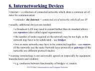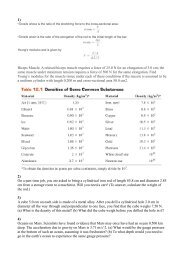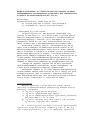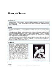
4th year Project demo presentation - Redbrick - DCU
4th year Project demo presentation - Redbrick - DCU
4th year Project demo presentation - Redbrick - DCU

You also want an ePaper? Increase the reach of your titles
YUMPU automatically turns print PDFs into web optimized ePapers that Google loves.
<strong>4th</strong> <strong>year</strong> <strong>Project</strong> <strong>demo</strong><br />
<strong>presentation</strong><br />
Colm Ó hÉigeartaigh<br />
CASE4 - 99387212<br />
coheig-case4@computing.dcu.ie<br />
<strong>4th</strong> <strong>year</strong> <strong>Project</strong> <strong>demo</strong> <strong>presentation</strong> – p. 1/23
Table of Contents<br />
An Introduction to<br />
Quantum Computing<br />
The Quantum Computing<br />
Language<br />
The Bloch Sphere<br />
The GUI<br />
Parallelizing the QCL<br />
<strong>4th</strong> <strong>year</strong> <strong>Project</strong> <strong>demo</strong> <strong>presentation</strong> – p. 2/23
An Introduction to<br />
Quantum Computing<br />
A qubit has two base states, denoted by the<br />
Dirac notation, |0〉 and |1〉.<br />
A qubit can be in a linear combination of<br />
states, denoted by;<br />
(1)<br />
|φ〉 = α|0〉 + β|1〉<br />
The power of quantum computing largely<br />
derives from two physical phenomena;<br />
superposition and entanglement.<br />
<strong>4th</strong> <strong>year</strong> <strong>Project</strong> <strong>demo</strong> <strong>presentation</strong> – p. 3/23
Superposition and<br />
Entanglement<br />
Superposition is the property of being able to<br />
exist in multiple states at the same time.<br />
Entanglement is a correlation between<br />
qubits that is stronger than any possible<br />
correlation in classical physics. An example<br />
is one of the Bell states;<br />
(2)<br />
|φ〉 =<br />
|00〉 + |11〉<br />
√<br />
(2)<br />
Bell states are used as the basis for quantum<br />
teleportation and super-dense coding.<br />
<strong>4th</strong> <strong>year</strong> <strong>Project</strong> <strong>demo</strong> <strong>presentation</strong> – p. 4/23
Quantum Algorithms<br />
The two most famous quantum algorithms<br />
are Shor’s Algorithm and Grover’s Algorithm.<br />
Shor’s algorithm can factor a large composite<br />
number that is the product of two prime<br />
numbers in polynomial time.<br />
Grover’s algorithm can search an<br />
unstructured database in quadratic time.<br />
<strong>4th</strong> <strong>year</strong> <strong>Project</strong> <strong>demo</strong> <strong>presentation</strong> – p. 5/23
Quantum<br />
Algorithms(2)<br />
Discovering new algorithms is complicated<br />
by the difficulty in getting the quantum state<br />
to decohere to the wanted values.<br />
It is also complicated by the fact that every<br />
operation in Quantum Computing must be<br />
reversible. This means any matrix used must<br />
be Unitary. This is a major restriction on what<br />
can be done.<br />
<strong>4th</strong> <strong>year</strong> <strong>Project</strong> <strong>demo</strong> <strong>presentation</strong> – p. 6/23
The future of<br />
Quantum Computing<br />
It is unclear as yet how powerful the quantum<br />
computing paradigm is. The fact that an NP<br />
problem such as factoring can be solved in<br />
exponential time is encouraging.<br />
The complexity space of the quantum<br />
computer is a subset of PSPACE, ie. those<br />
problems bounded on memory, but<br />
unbounded on time.<br />
It is probable Quantum Computing will solve<br />
a few more NP problems, and speed up the<br />
solution to many more.<br />
<strong>4th</strong> <strong>year</strong> <strong>Project</strong> <strong>demo</strong> <strong>presentation</strong> – p. 7/23
The Future(2)<br />
A useful Quantum Computer has never been<br />
built, due to the engineering difficulties<br />
involved in preventing the quantum state<br />
from decohering.<br />
A Quantum Computer was built in 2001 at<br />
IBM with 7 qubits, which <strong>demo</strong>nstrated<br />
Shor’s algorithm, factoring 15 into 5 and 3!<br />
<strong>4th</strong> <strong>year</strong> <strong>Project</strong> <strong>demo</strong> <strong>presentation</strong> – p. 8/23
The Quantum<br />
Computing Language<br />
The QCL is a programming language<br />
designed to approach quantum computing<br />
programming using the syntax of a<br />
procedural language like "C".<br />
It provides a base set of operators, yet is<br />
extremely powerful.<br />
The QCL contains a number of classical<br />
components such as if statements,<br />
for/while/until loops, functions, etc.<br />
<strong>4th</strong> <strong>year</strong> <strong>Project</strong> <strong>demo</strong> <strong>presentation</strong> – p. 9/23
The QCL(2)<br />
Qubits are manipulated by declaring<br />
quantum registers, qureg, with an arbitrary<br />
number of qubits. An operator can be<br />
applied to a quantum register.<br />
QCL defines many operators for quantum<br />
registers, among them; Rot(real theta, qureg<br />
q) and Mix(qureg q).<br />
<strong>4th</strong> <strong>year</strong> <strong>Project</strong> <strong>demo</strong> <strong>presentation</strong> – p. 10/23
The Bloch Sphere<br />
A qubit is normally represented as a linear<br />
combination of the basis states |0〉 and |1〉;<br />
(3)<br />
|φ〉 = α|0〉 + β|1〉<br />
This can also be represented as;<br />
(4)<br />
|φ〉 = cos θ 2 |0〉 + eiϕ sin θ 2 |1〉<br />
The numbers θ and ϕ in equation (2) define a<br />
point on the unit three-dimensional sphere.<br />
This sphere is called the Bloch Sphere.<br />
<strong>4th</strong> <strong>year</strong> <strong>Project</strong> <strong>demo</strong> <strong>presentation</strong> – p. 11/23
The Bloch Sphere(2)<br />
<strong>4th</strong> <strong>year</strong> <strong>Project</strong> <strong>demo</strong> <strong>presentation</strong> – p. 12/23
The Bloch Sphere(3)<br />
The Bloch Sphere provides a useful means<br />
of visualizing the state of a single qubit.<br />
However, there is no simple generalization of<br />
the Bloch sphere known for multiple qubits.<br />
A classical bit would be represented on the<br />
bloch sphere as being either at the north<br />
pole of the sphere or at the south pole.<br />
A qubit however, can be a point anywhere on<br />
the surface of the sphere.<br />
<strong>4th</strong> <strong>year</strong> <strong>Project</strong> <strong>demo</strong> <strong>presentation</strong> – p. 13/23
The Bloch Sphere(4)<br />
The latitude defines how close the qubit is to<br />
the poles, depending on the probability<br />
amplitudes.<br />
The qubit exists on every point on the<br />
longitude semicircle<br />
To draw the bloch sphere, the GNU libplot<br />
library is used. Libplot is a freely available<br />
C/C++ function library for<br />
device-independent 2-D vector graphics.<br />
<strong>4th</strong> <strong>year</strong> <strong>Project</strong> <strong>demo</strong> <strong>presentation</strong> – p. 14/23
The Bloch Sphere(5)<br />
The QCL uses GNU Bison and Flex to<br />
provide a correct syntax for the language.<br />
Bison is used in the QCL to ensure that<br />
whatever is typed in at the command line is<br />
syntactically correct in accordance with the<br />
grammar of the QCL.<br />
Flex is used to scan the input and to execute<br />
the corresponding C++ code.<br />
The semantics of the Bloch Sphere<br />
command are handled deeper in the code.<br />
<strong>4th</strong> <strong>year</strong> <strong>Project</strong> <strong>demo</strong> <strong>presentation</strong> – p. 15/23
The GUI<br />
The server program is designed to run on a<br />
Linux cluster and monitors the nodes<br />
dynamically. It packages this information in a<br />
class and broadcasts it to the client<br />
programs, which display the information<br />
graphically.<br />
The server program extracts information<br />
from the cluster by running and parsing<br />
various Linux commands.<br />
The client program displays the information<br />
dynamically, by querying the server every<br />
five seconds.<br />
<strong>4th</strong> <strong>year</strong> <strong>Project</strong> <strong>demo</strong> <strong>presentation</strong> – p. 16/23
The GUI<br />
The client uses the proxy pattern to contact<br />
the server, and the observer pattern is used<br />
on the server, to update the object the server<br />
broadcasts whenever the state of the cluster<br />
changes.<br />
The client application is embedded inside an<br />
application called WeirdX. WeirdX is a pure<br />
Java X Window System Server.<br />
It allows you to run a graphical application on<br />
a server machine and then to redirect the<br />
graphical output to another machine where it<br />
is displayed using WeirdX.<br />
<strong>4th</strong> <strong>year</strong> <strong>Project</strong> <strong>demo</strong> <strong>presentation</strong> – p. 17/23
Parallelizing the QCL-<br />
Motivation<br />
Simulating a quantum computer on a<br />
classical computer is a computationally hard<br />
problem.<br />
As the qubits in the quantum register are<br />
superposed with each other, the number of<br />
basevectos increases exponentially.<br />
Applying an operation to a quantum state is<br />
simply a matrix-vector multiplication.<br />
<strong>4th</strong> <strong>year</strong> <strong>Project</strong> <strong>demo</strong> <strong>presentation</strong> – p. 18/23
Parallelizing the<br />
QCL(2)<br />
The CA Linux cluster was used in this project<br />
for parallel computation in the QCL.<br />
The mpich implementation of the Message<br />
Passing Interface(MPI) library is used in this<br />
project.<br />
The number of nodes to run the program<br />
must be specified on the command line.<br />
QCL is allowed to execute normally on the<br />
head node, all other nodes are trapped<br />
inside a loop awaiting instructions from the<br />
head node.<br />
<strong>4th</strong> <strong>year</strong> <strong>Project</strong> <strong>demo</strong> <strong>presentation</strong> – p. 19/23
Parallelizing the<br />
QCL(3)<br />
Data is sent to nodes from the head node<br />
and gathered back in using different MPI<br />
operations.<br />
Various kinds of matrix-vector multiplication<br />
algorithms are implemented in the QCL.<br />
The Block-checkerboard partitioning<br />
algorithm sees the matrix being divided up<br />
into small squares of size (2x2). Each node<br />
gets a block and a portion of the vector.<br />
<strong>4th</strong> <strong>year</strong> <strong>Project</strong> <strong>demo</strong> <strong>presentation</strong> – p. 20/23
Parallelizing the<br />
QCL(4)<br />
The Self-Scheduling or Master-Slave<br />
algorithm broadcasts the vector X to each<br />
node, and the farms out one row at a time to<br />
all the nodes. This is inefficient due to the<br />
large amount of communication required.<br />
The Block-striped partioning algorithm<br />
stripes a matrix of size (n x n) row-wise<br />
among p processes, so that each processor<br />
stores n/p rows of the matrix.<br />
The next approach is combine the<br />
Compressed Sparse Row storage format<br />
<strong>4th</strong> <strong>year</strong> <strong>Project</strong> <strong>demo</strong> <strong>presentation</strong> – p. 21/23<br />
with the block-striped partioning approach.
Parallelizing the<br />
QCL(5)<br />
An efficient way of storing spares matrices is<br />
the CSR approach. Instead of a large<br />
rectangular array, three arrays are used to<br />
store the matrix. This greatly reduces<br />
communication overhead.<br />
The final approach uses block-checkerboard<br />
partitioning again, but it is more advanced<br />
than the first example, in that it only sends<br />
the vector portions to the head nodes of<br />
each column of the matrix, who then<br />
redistribute it down the column.<br />
<strong>4th</strong> <strong>year</strong> <strong>Project</strong> <strong>demo</strong> <strong>presentation</strong> – p. 22/23
Parallelizing the<br />
QCL(6)<br />
When all the results come back from the<br />
nodes, they need to be recombined, and the<br />
answer must be stored back in the original<br />
quantum register.<br />
<strong>4th</strong> <strong>year</strong> <strong>Project</strong> <strong>demo</strong> <strong>presentation</strong> – p. 23/23